Data Analytics Project - IDENTIFYING IRISH COUNTY WITH BEST QUALITY OF LIFE BSc(Hons) in Computing - NORMA@NCI Library
←
→
Page content transcription
If your browser does not render page correctly, please read the page content below

Data Analytics Project
IDENTIFYING IRISH COUNTY WITH BEST QUALITY OF LIFE

                       BSc(Hons) in Computing
                            Data Analytics
                              2020/2021
                              Mark Kelly
                              17138311
                     X17138311@student.ncirl.ie
Link to R Shiny Application: https://mrk-kelly.shinyapps.io/Project_app/
Data Analytics Project

Table of Contents
 EXECUTIVE SUMMARY ................................................................................................................................................................. 2
 INTRODUCTION .......................................................................................................................................................................... 3
    Background ...................................................................................................................................................................... 3
    Aims ................................................................................................................................................................................. 4
    Technology ....................................................................................................................................................................... 5
    Structure........................................................................................................................................................................... 6
 DATA....................................................................................................................................................................................... 7
    Data Selection .................................................................................................................................................................. 7
    Exploratory Analysis ....................................................................................................................................................... 15
 METHODOLOGY ....................................................................................................................................................................... 21
    Selection ......................................................................................................................................................................... 21
    Pre-Processing ................................................................................................................................................................ 22
    Transformation .............................................................................................................................................................. 26
 ANALYSIS ................................................................................................................................................................................ 41
    Data Mining ................................................................................................................................................................... 41
 RESULTS ................................................................................................................................................................................. 43
    Correlation Matrix .......................................................................................................................................................... 43
    Correlation Matrix with Significance Levels (p-value) .................................................................................................... 43
    Correlogram ................................................................................................................................................................... 44
    Rpart Decision Tree ........................................................................................................................................................ 45
    Random Forest ............................................................................................................................................................... 48
    Model Predictions........................................................................................................................................................... 49
    Best County Analysis ...................................................................................................................................................... 50
    Best County Testing ........................................................................................................................................................ 52
 CONCLUSIONS ......................................................................................................................................................................... 53
 FURTHER DEVELOPMENT OR RESEARCH ......................................................................................................................................... 54
 REFERENCES ............................................................................................................................................................................ 55
 APPENDICES ............................................................................................................................................................................ 57
 PROJECT PLAN ......................................................................................................................................................................... 57
 REFLECTIVE JOURNALS ............................................................................................................................................................... 58
    Introduction.................................................................................................................................................................... 59
    Journal ............................................................................................................................................................................ 60
 OTHER MATERIALS USED. ........................................................................................................................................................... 68
 APPENDIX 3................................................................................................................................................................................................... 69
 APPENDIX 4................................................................................................................................................................................................... 70
 APPENDIX 5................................................................................................................................................................................................... 71
 APPENDIX 6................................................................................................................................................................................................... 74
 APPENDIX 7................................................................................................................................................................................................... 75
 APPENDIX 8................................................................................................................................................................................................... 75
 APPENDIX 9................................................................................................................................................................................................... 76
 APPENDIX 10................................................................................................................................................................................................. 77
 APPENDIX 11................................................................................................................................................................................................. 78
 APPENDIX 12................................................................................................................................................................................................. 79
 APPENDIX 13................................................................................................................................................................................................. 79
 APPENDIX 14................................................................................................................................................................................................. 80
 APPENDIX 15................................................................................................................................................................................................. 81
 APPENDIX 16................................................................................................................................................................................................. 82
 APPENDIX 17................................................................................................................................................................................................. 82
 APPENDIX 18................................................................................................................................................................................................. 83
 APPENDIX 19................................................................................................................................................................................................. 85
 APPENDIX 20................................................................................................................................................................................................. 86
 APPENDIX 21................................................................................................................................................................................................. 86
 APPENDIX 22................................................................................................................................................................................................. 87
 APPENDIX 23................................................................................................................................................................................................. 87
 APPENDIX 24................................................................................................................................................................................................. 88
 PROJECT PROPOSAL – UPDATED DECEMBER 2020 ................................................................................................................................................ 89

                                                                                                                                                                           P a g e 1 | 95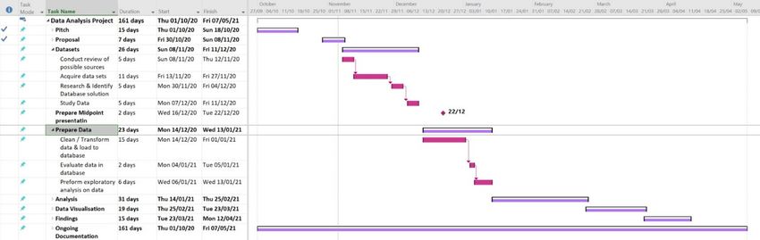
Data Analytics Project

Executive Summary

    The Covid-19 pandemic has led to several big employers like Indeed, Siemens, Twitter,
Salesforce & Spotify now allowing their employees to work remotely on a more permanent
basis. As more companies recognise the benefits of large-scale remote working (both for the
employee & employer), this list will grow as companies move from forced remote working to
smarter working in a post-Covid-19 environment. Large numbers of employees now no longer
must live in Dublin near their employer and are looking for alternative locations to call home.
    The project aim was to identify which county in the Republic of Ireland would offer the
best quality of life using variables that a typical family would consider. These variables include
crime rate, classroom size, property prices / monthly rent costs, distance to an emergency
department et cetera. These datasets are the most current available.
    The project also compares the actual number of crimes versus the predicted number of
crimes using decision trees and random forest algorithms for a sample of counties. The
purpose of this was to determine if the eight independent variables are sufficient to predict
crime rates. The random forest proved to be the most accurate but not accurate enough to
be considered a good model.
    The results from the analysis and associated charts/graphs show the top counties a user
should consider for relocation. When using all nine variables in making the decision, the
county with the best quality of life is Dublin. This prediction is not a true reflection of the best
county, as including all nine variables is unrealistic. A more realistic scenario is that only
selected variables would be needed for individual analysis. This option is explored in the
results section using a ‘R’ Shiny application.
   The ‘R’ Shiny application has been developed to allow users to pick the variables they
would like to include in the analysis. The county with the best quality of life will be computed.
Additionally, the application also provides summaries per county and per variable.

                                                                                  P a g e 2 | 95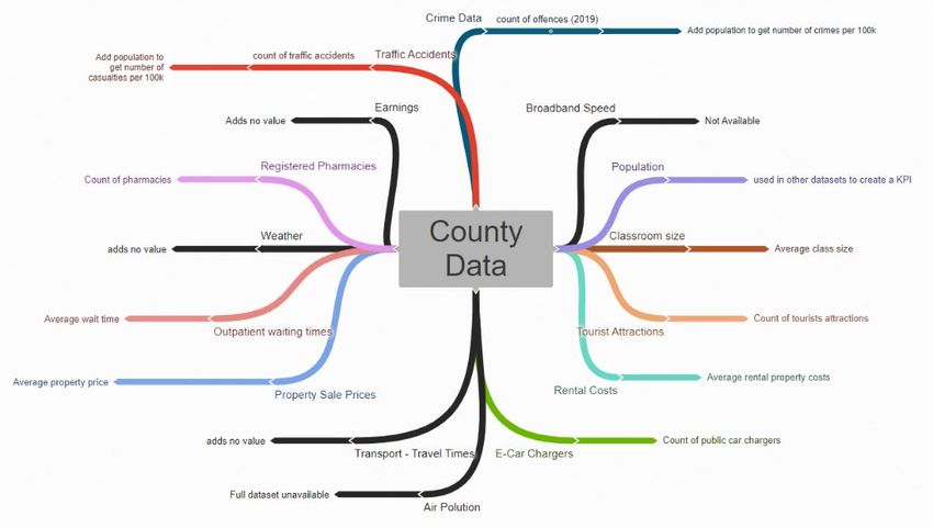
Data Analytics Project

Introduction

Background

    Before Covid-19, it was the norm to live in Dublin (or the commuter belt), near your Dublin
based employer. E-working or remote working was a factor for some employers, with a 2018
Blueface report finding that 78% of Irish companies had a remote working policy in place.
(78% of Irish businesses now have a Remote Working Policy in place Technology, news for
Ireland, Ireland, Technology, 2020)
    However, to look further into this, a research paper published in 2019 by the Department
of Business, Enterprise, and Innovation (Department of Business, Enterprise, and Innovation,
2019)was reviewed. This research paper investigated what defines remote working and
concluded it was either when employees worked from their homes or worked from a hub
close to or within their local community. The report discusses a pilot survey that the Central
Statistics Office (CSO) undertook in 2018. This pilot survey found 18% of respondents worked
from home, mostly one or two days per week.
    A Remote Work in Ireland Employee Survey was undertaken after this report addresses
the lack of data around employee participation in remote working. However, the sample was
considered skewed by a high response rate from the Finance and ICT sectors. Nevertheless,
while the survey is not fully representative and likely overstates remote work, it does offer
valuable insights. Some of these insights include:
           o Remote working is more common in the private sector (63%) than in the public
               sector (28%).
           o 48.5% of the respondents said they worked remotely.
           o Working remotely every week (part of a working week) was most common at
               51.1% compared to only 25.1% for the private sector & 10.1 % for the public
               sector who work remotely daily (every day)

    The arrival of Covid-19 had a sudden and dramatic impact on remote working in Ireland.
From March 16th, 2020, almost 100% of office-based work moved to remote working for both
the private and public sector.
   Many companies have now started to see benefits in allowing their staff to work remotely
on a more permanent basis, and these include Indeed (Indeed to allow 'vast majority' of Irish
employees to work from home forever, 2020) and Siemens (Kelly, 2020). They have both
opted to let their office-based workforce work remotely on a more permanent basis, as an
example.

                                                                              P a g e 3 | 95
Data Analytics Project

    This project was appealing as between April 2020 and August 2020, colleagues and family
friends relocated out of Dublin without changing jobs. At least one of these moves was to get
away from the high rents of Dublin, and Covid-19 provided the opportunity to keep their
current employment and move to a better location. Interestingly, the decision to move
developed quickly and how many other people are thinking like this, and where could they
move?

Aims

    In a post-Covid-19 environment, there will be a notable increase in the number of
employees availing of remote working in Ireland. With this project, the aim was to identify,
using the datasets selected, which county offers the best quality of life if a move from Dublin
(or anywhere else) is an option for those staff choosing to work remotely. The project
delivered by preparing the datasets, merging the data into a single data set, and then
normalising the data to make it comparable. Without any weighting, the county with the best
combination of variables was identified and then using only selected variables (this was to
simulate a real-world scenario, where not every variable will be necessary to all readers).
     In addition to this, the aim was to compare a selected variable from sample counties to
the output from a Random Forest and decision tree algorithms. The crime data was chosen
as the dependent variable that the models will predict. The crime variable was selected as of
all the variables, there will be readers that would not have an interest in the other variables
(e.g., short/medium term relocation would not be interested in property prices as they will
be renting, couples with no children would not be interested in classroom sizes), but crime
has the potential to affect all.
    The report will then compare the model prediction to the actual data to indicate how the
test counties are compared to the model prediction. The report will also compare the decision
tree and Random Forest results to identify which algorithm offers the best prediction.
    The report also includes a correlation heatmap to view correlations between the
variables.

                                                                              P a g e 4 | 95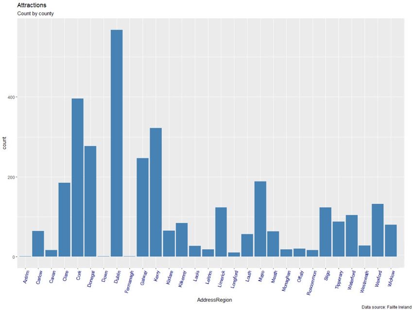
Data Analytics Project

Technology

    The primary language used for the analysis is the R programming language, with various
libraries within R required. The project proposal described the R programming language for
the pre-processing & transformation and then switching to Python for the analysis. Before
beginning the project, some further research was conducted, including a comparison on how
to do selected analysis in both languages using "Comparative Approaches to Using R and
Python for Statistical Data Analysis" (Rui and Vera, 2017), and a paper "MatLab vs Python vs
R ". (Colliau et al., 2017) After reviewing this a decision was made adopt the R programme
language for the whole project. R Studio is the integrated development environment (IDE) of
choice when using R, so this is the IDE that I will use. The R packages used are:
        o   Dplyr:                    Data manipulation.
        o   Ggplot2:                  Data visualisation.
        o   Readxl:                   Read Excel files.
        o   Tidyr:                    To tidy messy data.
        o   Dbplyr:                   Interact with databases.
        o   Rvest:                    Web Scrapper.
        o   Amelia:                   Missmap function to visualize missing data.
        o   Fuzzyjoin:                join data frames in R.
        o   Hmisc:                    compute the significance levels.
        o   PerformanceAnalytics:     to display a chart of a correlation matrix.
        o   Rsconnect :               Deploy and manage Shiny applications.
        o   Shiny:                    Interactive visualizations.
        o   Shinythemes:              Alter the overall appearance of Shiny applications.
        o   Rpart:                    Decision Tree algorithm.
        o   randomForest:             Random Forest algorithm.
        o   MLmetrics:                Calculate MAPE (mean absolute percentage error).
        o   Corrplot:                 Graphical representation of a correlation matrix.
        o   SP:                       Spatial data classes and methods (required for maps).
        o   Rgeos:                    Interface to Geometry Engine(required for maps).
        o   Maptools:                 Tools for Handling Spatial Objects.
        o   SQLdf:                    Manipulate data frames using SQL.

    Having reviewed several database options, the data was stored on an SQLite database,
and the associated R package (RSQLite) was used with the R programming language. SQLite
was chosen because its feature best suits the project. As a serverless application, it resides in
a single file, making it easy to move and share. It is also ideal for projects with a low amount
of requests, which this project will have.

                                                                               P a g e 5 | 95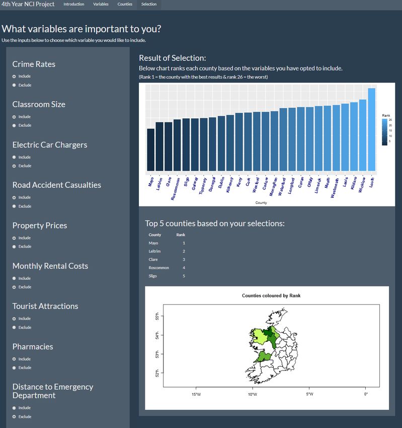
Data Analytics Project

    For the data mining element of the project both a decision tree and Random Forest
algorithms were implemented. The decision tree algorithm used is the Recursive Partitioning
(rpart) package in 'R'. The most commonly used decision tree algorithm is the C5.0 algorithm,
but this is used primarily for classification, whereas 'rpart' can be used either in regression or
classification. Random forest was added to this analysis as it is particularly well-suited to a
small sample size, which this analysis has.
    For the data visualisations, the project includes the Shiny package in R. This package will
allow interactive charts and graphs to allow end-users to interact with the data. In addition
to the programming of the Shiny application, HTML and CSS languages were used to
manipulate the presentation of the HTML pages that the Shiny Application generates.
    For the administrative side of the project, products from the Microsoft Office suite were
used. These include MS Project to develop and track the project timetable for the duration of
the project, MS OneNote to keep a record of keynotes and data references identified as the
project progressed, MS Word to produce this report and MS PowerPoint to create any slide
packs required to deliver mid-term and end of year presentations. MS Excel was used to
evaluate the datasets as they are acquired and as a second source when completing any
evaluation of the outputs from R Studio.
    Some of the datasets are sourced from the CSO, and their default format is PX. The PX
format is a standard format for statistical files used by statistical offices around the world. A
library in R (PC-Axis) can be used to read px files into R. PC-Axis was installed, and correct
syntax followed for the library 'pxR'. However, when trying to merge this data with other data,
errors occurred that were unresolvable. Following some research, an alternative method to
using this data was identified and the decision to install the Px Win software package
developed by the Swedish statistics office (Statistics Sweden, 2016) to read and convert the
data to an alternative format. The converted files were saved to ‘.CSV’ for convenience, which
allowed R to read the data and merge it with other data without any issues.

Structure

   The following is a brief overview of the document's structure and what is addressed in
each section.
   Methodology:        An overview of the methodology applied to the project, plus summary
                       details of each of the different stages that the project went through to
                       get from raw datasets to completed analysis, including the
                       transformation tasks required to get the data from raw to the required
                       state.

                                                                                P a g e 6 | 95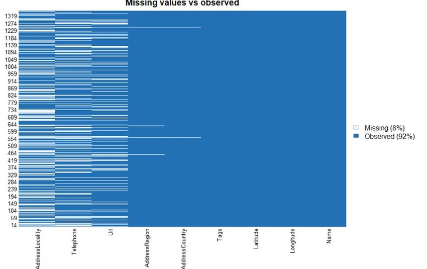
Data Analytics Project

    Data Selection:    Provides a summary of each of the datasets used in the project,
                       including their attributes, format of the raw dataset, and source of each
                       dataset.
    Transformation: Details on the steps taken to transform each dataset from its raw state
                    to the final state, ready to be used in the analysis.
    Analysis:          An overview of the approaches included in analysing the data and why
                       they were chosen. The report will also provide details on the essential
                       features of the analysis.
    Results:           Present the Interpretation and evaluation of the analysis.
    Conclusions:       Describe the advantages/disadvantages, strengths and limitations of
                       the project and its outcomes.
    Future:            Details of further development or Research that could be provided with
                       additional time and resources.

Data

   This section is divided into two. The first section presents the raw data, including a
description, its attributes, and its source. The second section will detail the exploratory data
analysis.

Data Selection

    This section provides a summary of each of the datasets used in the project. If a dataset
is not used in the project or the dataset used is different from planned, the blockers
encountered and why they were not overcome have been documented.

Name:           Recorded Crime Offences Under Reservation (Number) by Garda Station

Description:    This dataset is available in the ‘.PX’ format. The dataset contains a count of
                offences for the years 2003 – 2019 by the type of offence, Garda Station
                location, and regional division.

Attributes:     The raw dataset attributes are:

                                                                              P a g e 7 | 95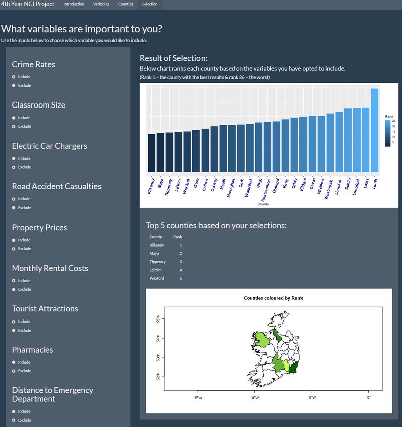
Data Analytics Project

                       File Format                CSV (initially .PX)
                       Data Format                Structured
                       Number of Columns          19 (All Chr)
                       Number of records (rows)   6,770

Source:        This data is sourced from Irelands open data portal and is published by the
               CSO. (CJA07 - Recorded Crime Offences Under Reservation (Number) by Garda
               Station, Type of Offence and Year - data.gov.ie, 2020)

Name:          Mainstream Primary Schools by Class Size

Description:   This dataset is available in the ‘.PX’ format. The dataset contains the number
               of children in every mainstream primary school class for all schools in the
               Republic of Ireland (the number of classes varies from 1 to 40 per school). The
               data is for the 2019 / 2020 school year and is summarised by the school.

Attributes:    The raw dataset attributes are:
                       File Format                CSV (initially .PX)
                       Data Format                Structured
                       Number of Columns          49 (8 x Chr & 41 int)
                       Number of records (rows)   3,106

Source:        This dataset is sourced from Irelands open data portal and is published by the
               CSO. (ED121 - Mainstream Primary Schools by Class Size, Teacher Size of
               School, Year and Statistic - data.gov.ie)

Name:          E-Car charger Network

Description:   The original source of this data was from Open Charge Map. (Open Charge
               Map - The global public registry of electric vehicle charging locations) Their
               dataset is Accessed via an API. However, the API is capped at 500 records, but
               there are many more chargers in the republic of Ireland. They do not have a
               premium API offering to obtain greater than 500 records, and the only filter
               option their API has is country.
                                                                             P a g e 8 | 95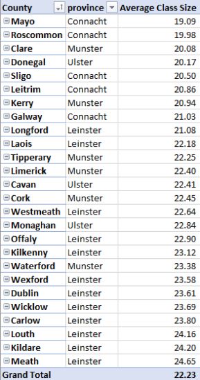
Data Analytics Project

               Contact was made with ESB E-cars, who very nicely supplied their current list
               of all chargers on their network in Ireland. The list is an immaculate list with
               charger name, address and charging speed. The problem is that ESB only
               accounts for approximately 65% of the public charging network. ('EasyGo |
               Charging Network', 2021) The other prominent provider in Ireland is EasyGo.
               When contacted, they were helpful, pointing to their website, which has a
               map (and list) of their charging network and the other providers.
               The data on their site is not downloadable, so the first attempt was to use a
               web scraper to extract the data using the 'rvest' package in R.
               The next problem encountered was that the list of chargers displayed on the
               screen reflected the area visible on the accompanying map. The effect of this
               feature meant a web scraper could not be used to extract the data, as each
               time the site opens, it uses IP's address’s current location to set the centre of
               the map, and if other areas of the country are required, the map must be
               moved manually. The second option was to zoom the map out to a province
               and copy the list displayed into an excel sheet. This approach worked, but the
               extracted data from the site needed some work to get it into a usable state
               (see pre-processing in the next section of the report).

Attributes:    The raw dataset attributes are:
                       File Format                CSV
                       Data Format                Semi-Structured
                       Number of Columns          1 Chr
                       Number of records (rows)   2,826 (5    per   charger
                                                  location)

Source:        This dataset is extracted from the website of a privately owned, public
               charging network operator. (‘EasyGo | Charging Network’, 2021)

Name:          Traffic Collisions and Casualties by County

Description:   This data is sourced from Irelands open data portal and is published by the
               Road Safety Authority. This dataset contains a single line summary per

                                                                              P a g e 9 | 95
Data Analytics Project
county with the number of collisions (both fatal & injury) and the number of
casualties (both fatal & injury).
Attributes: The raw dataset attributes are:
File Format CSV
Data Format Structured
Number of Columns 7 (1 x Chr & 6 x int)
Number of records (rows) 26 (1 per county)
Source: (ROA27 - Traffic Collisions and Casualties by County, Year and Statistic -
data.gov.ie, 2020)
Name: Average Earnings
Description: This dataset was deemed unnecessary as the premise of t analysis is based on
remote working, so earnings based on the county of residence are not valid
for the analysis.
Name: Broadband Speed
Description: Not for the lack of trying, but this dataset has been excluded from the analysis
as a source of this data was unavailable. Efforts were made to contact
comparison sites to obtain data, but the best that could be obtained was a
nationwide speed average. Contact with National Broadband Ireland (NBI) was
also attempted, they are responsible for the roll-out of the national broadband
plan, but no reply has been received at the time of writing. The alternative was
to use a dataset over four years old, which a decision was made not to do as a
lot has changed in the broadband domain in that period.
P a g e 10 | 95Data Analytics Project
Name: Property Sale Prices
Description: The dataset contains the sale price of every property sale (Jan – Nov 2020) in
the Republic of Ireland. This dataset was most recently updated on December
9th, 2020.
Attributes: The dataset attributes are:
File Format CSV
Data Format Structured
Number of Columns 9 (all Chr)
Number of records (rows) 40,353
Source: This data is published by the Property Services Regulatory Authority.
(Property Services Regulatory Authority, 2020)
Name: Transport – Travel Times
Description: It was decided not to add this dataset to the analysis as the topic centres
around remote working, and travel times would not be a factor.
Name: Weather
Description: This dataset was not pursued as it adds no value to the analysis, and no
additional insight would be gained from using it.
P a g e 11 | 95Data Analytics Project
Name: Tourist Attractions
Description: This dataset is available as an API GET call. The data set is loaded directly into
a data frame in R from the API. The dataset contains the name and address of
every tourist attraction registered with Failte Ireland.
Attributes: The dataset attributes are:
File Format API / Link to source
Data Format Structured
Number of Columns 8 (6 x Chr & 2 x num)
Number of records (rows) 3,324
Source: This dataset is sourced from Failte Ireland (Fáilte Ireland)
Name: Monthly Rental Costs
Description: This dataset reports on the average rent by location (e.g., town or area) and
county for the republic of Ireland. This dataset was most recently updated on
December 1st, 2020, with Q2 2020 data.
Attributes: The dataset attributes are:
File Format CSV
Data Format Structured
Number of Columns 7 (6 x chr & 1 x num)
Number of records (rows) 447
Source: This data is published by the Residential Tenancies Board (Residential
Tenancies Board, 2020) and was accessed via the CSO website.
P a g e 12 | 95Data Analytics Project
Name: Outpatient Waiting Lists
Description: The dataset contains the count of patients on an outpatient waiting list on
different dates during 2020. The most recent data will be used in the analysis.
The hospital summarises the data and contains a count by speciality,
adult/child grouping, age profile & time band (waiting time in months).
Attributes: The dataset attributes are:
File Format CSV
Data Format Structured
Number of Columns 10 (all Chr)
Number of records (rows) 55,969
Source: This data is published by The National Treatment Purchase Fund (OP Waiting
List by Group Hospital - OP Waiting List by Group Hospital 2020 - data.gov.ie,
2020) and was accessed via Irelands open data portal. This dataset was
updated on August 27th, 2020.
Name: Air Quality
Description: A full nationwide dataset on this subject was unobtainable, so Air Quality has
been removed from the analysis. The best data set I could locate was from the
EPA, but this was only available for cities.
Name: Registered Pharmacies
Description: The dataset contains the count of pharmacies by county, with Dublin split
into 25 (Co Dublin, Dublin 1 et cetera). The data was last updated on
December 1st, 2020.
P a g e 13 | 95Data Analytics Project
Attributes: The dataset attributes are:
File Format CSV
Data Format Structured
Number of Columns 2 (1 x Chr & 1 x int)
Number of records (rows) 50
Source: This dataset is published by the Pharmaceutical Society of Ireland and
available Irelands open data portal. (PSI Registered Pharmacies - December
2020 - data.gov.ie, 2020)
Name: Population count and density by county
Description: This dataset is for use in conjunction with other datasets to create additional
measures that can be used in the analysis.
Source: This dataset is sourced from Wikipedia (‘List of Irish counties by population’,
2020), with the population data confirmed by checking against the CSO
dataset. (Population at Each Census 1841 to 2016, 2020)
Name: Average Distance to Emergency Hospitals at ED Level
Description: This data was used in the CSO report, "Measuring Distance to Everyday
Services in Ireland". For emergency departments, the shortest-path analysis
was performed on hospitals where adult emergency care is provided. It was
last updated on February 17th, 2020.
This data set was added to the project after the outpatients waiting list data
set had to be excluded following the transformation tasks, which identified no
data for some counties in the Republic of Ireland.
P a g e 14 | 95Data Analytics Project
Attributes: The dataset attributes are:
File Format CSV
Data Format Structured
Number of Columns 12 (4 x Chr & 8 x int)
Number of records (rows) 3,410
Source: It is available via the geohive site. (Ordnance Survey Ireland, 2020)
Exploratory Analysis
The exploratory data analysis (EDA) will allow me to glimpse the general characteristics of
the dataset, which can be attained by generating descriptive statistics and data visualisations.
This analysis will be completed on the raw data sets to help summarise the data, find
outliers/anomalies, and identify interesting patterns. This analysis will also help identify what
actions need to be undertaken as part of the data transformation stage.
Crime Rate
The total number of reported crimes
(n=564) averaged 393 (s=971) per garda
station, per the 2019 data. The median
number of crimes per Garda station is 63,
indicating that the data set is positively
skewed (a more significant number of low
numbers). Figure 1 shows the spread by
Garda Station and the high number of garda
stations with low numbers.
Of the ten Garda Station with the highest
numbers, seven are in Dublin, with Pearse Figure 1
Street been the highest (10,210 crimes).
P a g e 15 | 95Data Analytics Project
Classroom Size
Some exploratory analysis using a ‘ggplot2’ column chart in ‘R’ shows students per county
(Appendix 14) using the totals column. All counties have some data, and there is no blank /
missing data. A check using 'summary' in R to verify that every
school had at least one classroom with students (Figure 2) was
also completed.
The number of students (n=3,106) averaged 22 (s=5) per
class in the current school year. The median number of
students per class is 22, indicating that the data set has a
symmetrical distribution. The histogram shown in Appendix 14 Figure 2
reflects this.
E-car chargers
The exploratory analysis for this data set was completed post-pre-processing and
transformation as the raw data was not in a condition that it could be analysed in any way.
The number of electric car chargers (n=26) averaged 49 (s=64) per county. The median
number of chargers per county is 49, indicating that the data set is positively skewed (greater
number of low numbers).
The bulk of the counties fall in the region of 24
chargers – 47 chargers (Figure 3), with only two
outliers (Cork & Dublin). A map chart can be
seen in Appendix 3.
Figure 3
Road Accident Casualties
Some exploratory analysis shows the number of casualties per county (Appendix 4). All
counties have some data, and there is no blank / missing data. Dublin stands out as the county
with a large number of casualties. The data will be normalised later to the number of
casualties per 100k population.
P a g e 16 | 95Data Analytics Project
The number of casualties (fatal & injured)
(n=26) averaged 305 (s=428) per county. The
range is large at 2,231, with one very high outlier
causing this (Figure 4).
Figure 4
Property sale prices
Exploratory data analysis completed with a histogram (R ggplot2) identifies a small
number of outlier sales over €1m (~1%). The outliers can be seen by looking at a histogram
of all sales (Appendix 5: All Property Sales). A second histogram with a more focused
perspective looking solely at the sales above €1m shows that a small number of the overall
sales are for a value greater than 1 million euro (Appendix 5).
Additionally, sales at the other end of the scale were also investigated. There are a small
number of sales below €50k also (Appendix 5). Using Google to research some of the below
€20k sales (full address of the property is available on the register) and some appear to be
residents buying out the local council's interest in a shared ownership scheme, I cannot find
any apparent reason for the others.
A decision was made to remove sales below €20k and above €1m from the dataset as they
will impact the average, but realistically very few properties will be sold in these two brackets.
The final nationwide population histogram shows a clear picture of the property sales in
2020 (Appendix 5) and using a facet wrap in ggplot to look at this by each county to make sure
good content can be seen.
Before removing the sales below €20k and above €1m, the sold property price (n=40,353)
averaged €310k (s=€1.1m). After removing the sales below €20k and above €1m, the sold
property price (n=39,512) averaged €265k (s=€160k). Interestingly, the mode of this sales
data is €150k (505 sales). The data set has a symmetrical distribution (skewness =1.3).
P a g e 17 | 95Data Analytics Project
Attractions
Figure 5
Exploratory data analysis completed with a bar chart (R ggplot2) to count the number of
attractions by the county has identified that there are a small number of attractions where
the address does not include a county (Appendix 6) and confirmed by counting NAs in R
(Figure 5).
These will need to be resolved in the transformation of this dataset before moving on.
Rental Costs
Initial exploratory analysis shows that there are 47 locations with no average rental value
(see appendix 9 & figure 6)
Figure 6
The monthly rental amount (n=447) averaged €1,193 (s=€484) across all locations and all
property types. The median rental amount is €1,111, indicating that the data set has a
symmetrical distribution (skewness = 0.52). The histogram shown in Appendix 9 reflects this.
Outpatient waiting list
Initial review of data shows only one missing record (Figure 7) from this large dataset.
This missing record is in the ‘Time Bands’ column, which I will investigate and update if
required, as I will use this column to measure the average wait time.
Figure 7
P a g e 18 | 95Data Analytics Project
The dataset has multiple records for each key date, and as only the most recent data will
be used in the analysis, all other key dates will be removed from the dataset. In addition to
this, it has been decided to split this data set into multiple data sets:
Adult - Waiting time
Adult - Count on waiting list
Child - Waiting time
Child - Count on waiting list
An initial summary of the raw data shows
that there are 611k patients on the outpatient
waiting list on 27/08/2020, and ~14% of these
are children (Figure 8). There will be further
analysis done on this data set after
transformation.
Figure 8
Registered Pharmacies
Exploratory data analysis completed with a bar chart (R ggplot2) to count the number of
registered pharmacies by the county has identified that County Dublin data has been split into
different areas. (Appendix 10). These will need to be resolved in the transformation of this
dataset before moving on. There is also a “Grand Total” dimension that will also need to be
removed.
P a g e 19 | 95Data Analytics Project
Population
Census 2016 population data
were used to derive new measures as
well as normalise data sets. The total
population is 4.7m, and a county by
count breakdown can be seen in
Figure 9.
Figure 9
Distance to an Emergency Department
A review of the data in R shows that there are no missing values (Figure 10).
Figure 10
Data is by location, with 3,409 location across the 26 counties. Distance to an ED is in a
range format, and this will need to be converted to a kilometre value in the transformation
stage.
Location Count
Less than 5km 397
5 - < 10km 263 An initial count shows that the 25km – 50km
10 - < 25km 918 range is the most common (Figure 11).
25 - < 50km 1410
Further analysis will be completed after the
50km or more 421
data is transformed.
Grand Total 3409
Figure 11
P a g e 20 | 95Data Analytics Project
Methodology
The methodology I used for this project is KDD (Knowledge, Discovery & Data Mining).
This methodology is a core data analytics methodology and is best suited to this data analysis
project. As KDD is an iterative process, outcomes can be refined, and conclusions can be
enhanced as the data is transformed, allowing for more relevant results. This iterative process
will benefit the project as each of the datasets will be evaluated initially and again as they are
merged into a larger dataset and can be tweaked or modified to allow for better integration
into the analysis.
The five stages of KDD are:
Interpretation /
Selection Pre-Processing Transformation Data Mining
Evaluation
In addition to this, a published journal on Domain Knowledge in the initial stages of KDD
(Szczuka et al., 2014) highlights the benefits of the overall analysis by increasing domain
knowledge on the data subjects. With this in mind, there is time incorporated into the project
data selection stage to study the data to be familiar with the data subjects before proceeding.
Selection
To identifying the datasets for the analysis, the first task was to identify the question that
was to be answered.
“If moving from Dublin (or anywhere else),
which county would offer the best quality of life?”
The next step was to look at what data would help answer this question, focusing on
datasets that a typical family would consider noteworthy. The resulting list of twenty datasets
was further whittled down to fifteen after some high-level research. The remaining datasets
(Figure 12) are, in my opinion, datasets that would add the best value to my analysis and
would be of interest to the report readers.
Full details of each data set can be found in Data Selection (section 2) of this report.
P a g e 21 | 95Data Analytics Project
Figure 12
Pre-Processing
The pre-processing stage consisted of cleaning and preparing the raw data to obtain
consistent, tidy data. Having read Hadley Wickham's paper on tidy data (Wickham, 2014) and
applied the four main principles to my pre-processing:
1. Each attribute (variable) should be in its own column.
2. Each observation should be in a different row.
3. One table per topic
4. When using multiple tables, they should have a column in common (primary key)
As most of the data was clean when acquired, there was minimal cleansing, although
some restructuring was required. An individual R file for each data set made it easier to
manage and save the processed data to the database when complete.
This section provides details of the pre-processing work carried out on each dataset
before beginning the transformation work.
The following data sets were sourced from the CSO via Irelands Open Data Portal
(Data.gov.ie, no date) in the ‘.PX’ format.
• Recorded Crime Offences Under Reservation (Number) by Garda Station
• Mainstream Primary Schools by Class Size
This format requires the PxWin software package developed by the Swedish statistics
office (Statistics Sweden, 2016) to read and convert to alternative formats. The software has
converted these files to '.CSV' for convenience.
P a g e 22 | 95Data Analytics Project
Below is a high-level summary of the actions taken to tidy the data for each dataset:
Data Set Details of pre-processing
Recorded Crime Offences Check for missing data using Missmap (see Appendix
8) & sapply (sum NAs)
Remove crime data for years 2003 – 2018 as only
data for 2019 was used in the analysis.
Some Garda divisions are spread over two counties,
and there was a requirement to split these into their
respective counties Details below (2)
Primary Schools by Class Size Check for missing data on key fields and at least one
classroom for each school using Missmap (Appendix
14) & sapply (sum NAs)
Remove unrequired columns from the data set.
• Roll Number
• Academic year
• School Address (excluding county)
• Eircode
• Local Authority
E-Car charger Network Pease next paragraph (1) below for details on
conversion from raw data
Check for missing data using Missmap (Appendix 3) &
sapply (sum NAs)
Traffic Accident Casualties Check for missing data using Missmap (Appendix 4) &
sapply (sum NAs)
Property Sale Prices Check for missing data using Missmap & sapply (sum
NAs) (Appendix 5)
The price variable was in a character format
containing ‘€’ & ‘,’ symbols (e.g., €120,000.00).
These needed to be removed using lapply and gsub
functions in R.
Variable converted to an integer.
Unwanted columns were removed.
• Date of Sale
• Address
• Postal Code
• Property Description
• Size Description
P a g e 23 | 95Data Analytics Project
Data Set Details of pre-processing
Tourist Attractions Check for missing data using Missmap & sapply (sum
NAs) (Appendix 6)
• 3 x attractions with missing county details.
• ‘which(is.na) function used to find indexes of
missing counties.
• Google attraction to find the county of
attraction.
• Added county to the data set.
Remove unwanted columns.
• Name
• URL
• Telephone
• Longitude & Latitude
• Address Locality & Country
Monthly Rental Costs Check for missing data using Missmap & sapply (sum
NAs) (Appendix 9)
• Found observations (47) with no average
monthly rent cost
Outpatient Waiting Lists Check for missing data using Missmap & sapply (sum
NAs) (Appendix 11)
• 1 Time band was found to be missing.
• ‘which(is.na) function used to find indexes of
missing time band.
• When viewed, this was for a key date other than the
date I planned to use – ignored.
Removed observations for all archive dates other
than the most recent (27/08/2020)
Registered Pharmacies Check for missing data using Missmap & sapply (sum
NAs) (Appendix 10).
Convert X variable (Count of pharmacies) to integer.
Population counts and density Remove the ‘,’ symbol from the population variable
by county and convert it to an integer.
Check for missing data using Missmap & sapply (sum
NAs) (Appendix 12)
Convert variables to an integer.
Remove Northern Ireland counties from the data
set.
Rename columns.
Average Distance to Emergency Check for missing data using Missmap & sapply (sum
Hospitals NAs) (Appendix 13)
Removed unwanted columns.
• FID & ObjectID
• ED Name
• Shape Area & Length
P a g e 24 | 95Data Analytics Project
(1) As mentioned in the above data selection section, the E-Car charging network data
was troublesome to get. After contacting a couple of sources, the EasyGo website was
identified as having a map (and list) of their charging network and the other providers in
Ireland. However, extracting this data was not straight forward.
The first attempt to obtain the data was using the 'rvest' library in R to scrape the page,
but this failed to read the list because the table has been dynamically generated based on the
area of Ireland shown in the accompanying map. That was verified by using the CSS Selector
Gadget Chrome addon.
The solution was to copy the displayed table in four sections (one for each province as this
was the most significant area that the map could zoom out to). Each section was then
concatenated together in MS Excel.
The resulting list in Excel
was all in a single column, with
five rows per charger location. A
combination of lookups,
concatenate, index & match and
substitute formulae allowed the
data to be converted into a
usable table (Figure 13).
Figure 13
(2) To complete the analysis, the data set had to be modified as the sum of crimes is by
Garda Station, including the Garda station location and division. There are 115 garda stations
(total = 564) that their county could not quickly be identified as their division is spread out
over two counties.
Division
Laois/Offaly Division
Cavan/Monaghan Division
Roscommon/Longford Division
Sligo/Leitrim Division
Kilkenny/Carlow Division
Laois/Offaly Division
An attempt was made to source a dataset/list of garda stations and their complete
address, but the CSO dataset containing this has been discontinued. The garda website was
also checked, but this uses a map feature or a search by division option. The data on Wikipedia
was examined as a possible source but was found to be incomplete.
P a g e 25 | 95Data Analytics Project
The solution was to create a list in ‘R’ that could be used to look up the details needed
(sourced from Wikipedia & Google) and merged it with my dataset using an inner join function
in ‘R’. A new subset was then created, which uses the amended division (single county).
Transformation
For the project, transformation involved converting each dataset from its raw state (post-
pre-processing) to an appropriate state to perform my analysis. This transformation included
the alignment of each dataset to a universal unit of measure (County) and ensuring the
required metric is correctly calculated before the datasets were merged. Additional measures
were also calculated to normalise the data, plus each data set was ranked.
The tasks required were identified in the earlier data pre-processing stage and the
exploratory analysis for each data set. After completion, each data set was saved to the SQLite
database.
Crime Data
Figure 14
Figure 14 shows a snapshot of the raw data before the transformation. The transformation of
the crime dataset into the required state, the following tasks were completed:
o Using aggregate, sum up the count of offences by Garda station.
o Using amended division column, identify which county each Garda station is located.
Create a vector that contains each county.
Use a 'For' loop to search through the Division column and use 'grepl' to
compare counties' vector to find the appropriate county (Figure 15).
Figure 15
P a g e 26 | 95Data Analytics Project
o Using aggregate, sum up the count of offences by county.
o Data merged with population dataset using 'inner join' function.
o The number of crimes per 100k population calculated.
o Normalise function applied to crimes per 100k population (Appendix 17).
o The rank column created referencing normalised data.
Classroom size
Figure 16
The transformation of the classroom data from raw (Figure 16 – before pre-processing)
into the required state, the following tasks were completed:
o Calculate the average classroom size per school – using
‘rowMeans’ in R.
o Calculate the average classroom size per county - using
‘aggregate’ in R.
o Normalise function applied to average class size (Appendix 17).
o The rank column created referencing normalised data.
To validate the calculation performed in R, MS Excel was used to generate
a pivot table (Figure 17) calculating the average classroom size per school
and compared this to the R output for a sample population. This validation
found no errors. Figure 17
Interestingly, all counties in Leinster except two (Longford & Laois) have
an average classroom size more significant than the national average.
E-car chargers
The transformation of the electric car charger data into the necessary state required the
following tasks were completed:
o Calculate the total number of car chargers per county - using ‘aggregate’ in R.
o Using the population data set, merge kilometres square size for each county
o Calculate the number of chargers per 100 km2.
o Normalise function applied to chargers per 100 km2 (Appendix 17).
o The rank column created referencing normalised data.
P a g e 27 | 95Data Analytics Project
Traffic Accidents Casualties
Figure 18
The transformation of the traffic accidents data from raw (Figure 18) into the necessary
state, the following tasks were completed:
o Remove all columns other than “All killed & injured casualties”.
o Merge with population data using the 'inner join' function.
o Calculate the number of casualties per 100k population.
o Normalise function applied to casualties per 100k (Appendix 17).
o The rank column created referencing normalised data.
A summary in ‘R’ after data transformation shows that the average casualties (includes
killed and injured) per county is 305. When this is normalised, the average per county is 172
per 100k population (Figure 19).
Figure 19
Some further exploratory analysis after transformation using a ‘ggplot2’ bar chart, we can
see which counties are above the average and below the average. Interestingly, Dublin is the
county closest to the average (Appendix 4).
Property Sale prices
Figure 20
P a g e 28 | 95Data Analytics Project
The transformation of the property sale price data (Figure 20 shows a sample of raw data)
into the requisite state needed the following tasks to be performed.
The exploratory analysis identified some outliers that will be removed to make the data
more useable, and these include all sales above €1m and all sales
below €20k.
o Remove outliers identified in exploratory analysis.
Figure 21 is a summary post removal of the outliers.
o Calculate the average sale price per county using the
aggregate function. Figure 21
o Format value to currency as a new column
o Remove decimal places.
o Normalise function applied to the average sale price (Appendix 17).
o The rank column created referencing normalised data.
Following the transformation of this dataset, the final output from a ggplot2 bar chart can
be seen in appendix 5: Average property sale price per county.
Attractions
Figure 22
The transformation of the attraction’s dataset into the required state (Figure 22 – sample
of the raw data set) required that the following tasks to be completed.
o The number of offences by county was calculated using the aggregate function.
o Using the population data set, merge kilometres square size for each county
o Calculate the number of attractions per 100 km2.
o Normalise function applied to attractions per 100 km2 (Appendix 17).
o The rank column created referencing normalised data.
Post transformation bar chart can be seen in Appendix 7: Count of Failte Ireland
Attractions per County
P a g e 29 | 95Data Analytics Project
Rent Costs
Figure 23
The transformation of the rental price dataset into the required state (Figure 23 – sample
of the raw data set) required the following tasks to be completed. The exploratory analysis
identified that 47 observations have no average rent. In reviewing the locations without a
value, there are other locations in the affected counties with values (e.g., Waterford has 21
locations, including an overall average for Waterford on the report). The easiest solution is to
remove all locations except the overall county average.
o Remove observations for all but overall county average values (Figure 24)
Create a vector that contains each
county.
Use a 'For' loop to compare counties'
vector to find the appropriate
county.
The new county column was then
used to compare to the location
column and remove any observations Figure 24
where the two columns did not
match.
o Remove columns other than county and rent.
o Copy value column to new column “average” and convert to currency (for use in
charts)
o Normalise function applied to average rent cost (Appendix 17).
o The rank column created referencing normalised data.
Following the data transformation, a ‘ggplot’ bar chart shows the average rental value per
month per county, with a horizontal line added to show the nationwide average (Appendix
9). Dublin has the highest rental cost, with Laois the closest country to the average.
P a g e 30 | 95You can also read