Data-Driven Air Quality Characterization for Urban Environments: A Case Study - ORCA
←
→
Page content transcription
If your browser does not render page correctly, please read the page content below
SPECIAL SECTION ON ADVANCED SOFTWARE AND DATA ENGINEERING FOR SECURE SOCIETIES

Received November 5, 2018, accepted November 21, 2018, date of publication December 3, 2018,
date of current version December 31, 2018.
Digital Object Identifier 10.1109/ACCESS.2018.2884647

Data-Driven Air Quality Characterization for
Urban Environments: A Case Study
YUCHAO ZHOU 1 , SUPARNA DE 1 , (Member, IEEE), GIDEON EWA2 ,
CHARITH PERERA 3 , (Member, IEEE), AND KLAUS MOESSNER 1 , (Senior Member, IEEE)
1 Institute for Communication Systems, University of Surrey, Guildford GU2 7XH, U.K.
2 Department    of Electronic Engineering, University of Surrey, Guildford GU2 7XH, U.K.
3 School   of Computer Science and Informatics, Cardiff University, Cardiff CF24 3AA, U.K.
Corresponding author: Suparna De (s.de@surrey.ac.uk)
This work was supported by the European Commission, Horizon 2020 Programme, TagItSmart! Project, under Contract 688061.

   ABSTRACT The economic and social impact of poor air quality in towns and cities is increasingly being
   recognized, together with the need for effective ways of creating awareness of real-time air quality levels
   and their impact on human health. With local authority maintained monitoring stations being geographically
   sparse and the resultant datasets also featuring missing labels, computational data-driven mechanisms are
   needed to address the data sparsity challenge. In this paper, we propose a machine learning-based method to
   accurately predict the air quality index, using environmental monitoring data together with meteorological
   measurements. To do so, we develop an air quality estimation framework that implements a neural network
   that is enhanced with a novel non-linear autoregressive neural network with exogenous input model,
   especially designed for time series prediction. The framework is applied to a case study featuring different
   monitoring sites in London, with comparisons against other standard machine-learning-based predictive
   algorithms showing the feasibility and robust performance of the proposed method for different kinds of
   areas within an urban region.

   INDEX TERMS Air quality estimation, air pollution, machine learning prediction, neural network.

I. INTRODUCTION                                                                                  activities with toxic air in towns and cities across the
With the growing population of the world and the migra-                                          UK. Poor air quality has clear public health impacts, with
tion of people to urban areas [1], it becomes imperative to                                      40,000 deaths annually in the UK (9,500 in London) directly
create an intelligent and sustainable environment that offers                                    attributable to air pollution and exacerbating health condi-
citizens a high quality of life and is geared towards sup-                                       tions with those with heart or lung conditions [3]. Spikes in air
porting their well-being. The direct effect of this urban drift                                  pollution levels have also been directly linked with increased
has had profound effects on social, economic and ecological                                      hospital and GP visits [4], pointing to additional costs faced
systems, causing stresses on the environment and society.                                        by the public health service in treating conditions exacerbated
The social and economic implications include impacts from                                        by poor air quality. This calls for effective ways of creating
human activities such as transport, industrialization, combus-                                   awareness of real-time air quality levels and their impact on
tion, construction etc., all of which have a direct or indirect                                  human health.
bearing on the environment. These pollution sources have                                            Since air pollution is highly location dependent [2] and
led to release of pollutants such as Nitrogen dioxide (NO2 ),                                    air quality monitoring sensors installed at fixed-site sta-
Particulate Matter (PM), Sulphur dioxide (SO2 ) etc. into the                                    tions, though very accurate, have high installation costs, are
atmosphere.                                                                                      bulky and geographically sparse (the UK’s DEFRA Auto-
   It is recognized that air pollution is influenced by urban                                    matic Urban and Rural Monitoring Network (AURN) has
dynamics [2]. Recent media reports1 have highlighted the                                         168 sites covering the entire UK [5]), this poses challenges for
links between road traffic and large-scale construction                                          evidence-based real-time air quality-related decision making,
                                                                                                 both for city authorities and citizens. Secondly, the data from
  1 https://www.theguardian.com/environment/2018/aug/28/too-dirty-to-                            these monitoring stations has lots of missing labels due to the
breathe-can-london-clean-up-its-toxic-air                                                        maintenance schedules of the devices in the station [6].
                                             2169-3536 2018 IEEE. Translations and content mining are permitted for academic research only.
77996                                              Personal use is also permitted, but republication/redistribution requires IEEE permission.        VOLUME 6, 2018
                                            See http://www.ieee.org/publications_standards/publications/rights/index.html for more information.
Y. Zhou et al.: Data-Driven Air Quality Characterization for Urban Environments: A Case Study Since there are a large number of air pollutants, which can and previous pollutant values. The selected AQI calculation combine actively or reactively to form secondary pollutants, model also proposes and evaluates two approaches for AQI countries have adopted the Air Quality Index (AQI) as a characterization and prediction: the first of which trains the measure of pollutants in the air. It is an easily understandable NARX algorithm directly on the calculated historical AQI value that shows how polluted the air is or how polluted it values, and the second predicts individual pollutant values will be in future. This information can be used to warn the before feeding them into the AQI calculation model. Eval- public or sensitive groups about the state of pollution of the uations based on a real-world dataset, and comparison to environment. the state-of-the-art methods in terms of standard evalua- Beginning with the first use in Toronto in 1969, AQI cal- tion metrics, i.e., Root Mean Squared Error, Mean Absolute culation and prediction has gained popularity and is widely Percentage Error, and Band Accuracy, show the feasibility adopted by many countries [7]. The complexity and number and performance improvements achieved from the proposed of factors affecting the AQI has motivated the use of computa- approach. tional intelligence techniques in the prediction of air quality, The rest of the paper is organized as follows. Section 2 pro- achieving higher accuracy than statistical methods such as vides a review of the related work and techniques for AQI moving average or linear or Gaussian interpolation [8]. The and pollutant estimation. The details of the AQI calculation emerging paradigm of urban computing [9], which aims to model and meteorology factors characteristics are described analyze the correlations and patterns from urban big data in Section 3. Section 4 presents the AQI estimation frame- to infer unknown knowledge [10], has researched various work, including algorithmic details of the NARX predictive aspects of air pollution, for instance, by employing data- model. Section 5 presents the experiments performed on a informed air quality prediction algorithms (to mitigate the dataset collected from a real-world deployment of monitoring data sparsity challenge [11]), with the developed Machine- sites across several boroughs of the city of London and also Learning (ML)-based algorithms achieving a high perfor- discusses the evaluation results based on the standard metrics mance in terms of the prediction accuracy and efficiency by comparing to existing methods. Section 6 concludes the [8], [12], [13]. Most of these research works implement paper and outlines the future research directions. techniques to predict and identify patterns relevant to indi- vidual pollutant concentrations, for example, PM2.5 [6], [14], II. RELATED WORK Carbon Monoxide (CO) [12], [13], [15], PM10 [8], [16] Prediction of air quality levels is important for communi- and Nitrogen Oxides (NOx ) [8], [15]–[17]. Other allied cating pollution risks and exposure level. However, it is works seek to employ supervised methods that take into a complex measure to calculate since the form and dis- account historical AQI values in order to perform short-term persal patterns of pollutants are affected by environmental predictions of AQI measures for the same or neighboring and meteorological factors. The early approach was human- regions [18], [19]. centered, where data collected from different monitoring However, it has been noted that there should be three stages stations were evaluated based on human experience; hence, involved in predicting AQI [20]: 1) establishment of an Air making it unreliable. Currently, computational intelligence quality model, 2) identification of meteorology factors and approaches involve use of smart algorithms such as decision forecast, and 3) doing the actual AQI forecast and estimation trees, neural networks, self-organizing maps, support vec- based on identified algorithms. The AQI calculation model tor machines etc. in predicting air quality. This method is choice is important since pollutants vary from place to place, advantageous because of its high accuracy and computational for example, an urban area may be concerned about NO2 efficiency [21]. because of large vehicular presence, an industrialized area Zhang et al. [22] identified the major techniques for AQI might want to monitor SO2 and a city like Madrid may be forecasting to include simple empirical approach and statisti- interested in pollen because of its prevalence in this region. cal approach. The empirical approach is based on persistence, Thus, the AQI model needs to consider individual pollu- which factors in current AQI into the prediction of future tants or a combination of them. Meteorology is an influenc- AQI since it assumes that the current pollutant value has a ing factor since it has been established that factors such as direct effect on tomorrow’s predicted value. This approach temperature, atmospheric pressure, relative humidity, wind is simple and good for stationary conditions but can’t handle speed and wind direction are dominant factors that influence sudden changes in pollutant and weather. Statistical approach pollutant concentration and by extension AQI [16]. relies on the fact that weather and pollutant concentrations are To implement the requisite three phases and to address the related statistically i.e. there is correlation between these two data sparsity and unlabeled data challenges, this paper sets out elements and therefore regression and trained neural network a comprehensive air quality estimation framework that imple- functions are employed to forecast pollutant concentration. ments an AQI model encompassing a predictive algorithm for air quality index, given pollutant and meteorology data. A. MACHINE LEARNING-BASED APPROACHES The novel predictive method applies the Non-linear Autore- Zhang et al. [22] mention the common algorithms to include gressive neural network with exogenous input (NARX) time Classification And Regression Tree (CART), Artificial Neu- series prediction model that considers meteorological inputs ral Network (ANN), and fuzzy logic. Their work noted that VOLUME 6, 2018 77997
Y. Zhou et al.: Data-Driven Air Quality Characterization for Urban Environments: A Case Study

ANN has fast computational speed and an ability to learn and            neural network-based approach in [14] uses a spatial trans-
adapt itself to new instances. Moustris et al. [15] applied an          formation component for spatial correlation and a distributed
ANN model for short-term forecasting of SO2 , NO2 , Ozone               fusion network to merge all the influential factors for PM2.5
(O3 ) and CO levels across seven monitoring sites in Athens,            forecasting.
with evaluation statistics showing a good agreement between
predicted and observed pollutant values. The study concluded            C. URBAN COMPUTING APPROACHES
that ANN can be used effectively for time series prediction             Allied research on transport-related themes has considered
and is optimized for problems with big state variables or large         the impact of weather changes on predicting traffic levels
dimensions. Hourly concentration of NO2 and NO and mete-                at different points in a city [23], and predicting transport
orology were used in [17] to forecast their values using neural         carbon emissions within a city [24]. Recent studies have
network and Support Vector Machine (SVM), with SVM’s                    explored urban models to predict air quality in city districts
ability to set the size of the hidden layers automatically pro-         by considering a range of spatio-temporal urban big data
viding better performance than ANN. Another finding from                sources such as meteorology, vehicular traffic and points of
this was that factor-less prediction i.e. prediction without            interest (POI) [2]. It is worth noting that different cities and
external variables, is fine but additional external variables           their public spaces are characterized differently based on their
greatly improve prediction. The downside of this is that if             specific natural and built environment [23], which needs to
the external variables are predicted, then it could worsen the          be considered while calculating and predicting the pollution
performance of the algorithm due to accumulated prediction              index and discovering the latent temporal and spatial patterns.
error. The use of ANN for hourly prediction of pollutants                  From the review of existing works, it is apparent that
was also demonstrated in [16], with known pollutant con-                several authors have used neural networks in their work to
centration values at 1, 2 and 3 hour, respectively, prior to            model and predict air quality and pollutant concentration. The
the prediction, used to approximate the impact of background            choice of this machine learning algorithm is strongly based
factors such as industrial, restaurant and resident emissions.          on its fast-computational attributes and its ability to learn and
This method was used to predict pollutant concentrations                adapt to new instances. Hassan and Li [25] noted that air
an hour in advance. Comparison of this ANN-based method                 quality prediction has complex and non-linear patterns. These
with multiple linear regression models shows that regression            patterns of data can be efficiently handled by neural networks.
models perform better for predicting CO and PM10 values,                Additional features in air quality prediction increase the
with mixed results for NO2 (comparable performance) and                 dimension of data, and Hassan and Li [25] stated that ANN is
O3 (ANN performs markedly better). The authors also intro-              naturally suited for problems with large number of state vari-
duced an ‘unknown-background’ ANN method, where the                     ables. Neural networks’ ability to make generalizations given
predicted concentrations were used as background factors                an input and its non-mapping capability makes it a good tool
for the following hour prediction, resulting in improved per-           for time series prediction. Thus, in this work, we explore a
formance for the ANN method. Grid-based forecasting of                  neural network-based algorithm and incorporate a time delay
PM10 levels using ANN for a spatial classifier that co-trains           to take into account prior pollutant concentrations into the
a semi-supervised model with spatial features such as points-           prediction of future AQIs. Compared to the existing works,
of-interest density and highway length, was used in [8]. This           our work considers all individual pollutant concentrations to
was extended with a temporal classifier based on conditional            provide a comprehensive AQI characterisation and prediction
random field that considered temporal features such as traffic          framework.
and meteorology. To address the problem of data sparsity
from geographically sparse air quality monitoring stations              III. BACKGROUND
installed by government agencies, HazeEst [13] and the work             In this section, we first establish the adopted AQI calculation
in [12] combined the data from static sites with mobile sensor          model, setting out how to calculate Air Quality Index (AQI)
data to forecast CO values for the metropolitan area of Sydney          based on the collected dataset. The characteristics of the sens-
by training and evaluating a number of regression models.               ing sites that are used as the data sources are then presented
Their findings show that SVR has the same estimation accu-              and analyzed. Then we present the statistics of the collected
racy as decision tree regression, but higher than multi-layer           meteorological and pollution data.
perceptron and linear regression.
                                                                        A. AQI CALCULATION
B. DEEP LEARNING APPROACHES                                             This section sets out the adopted AQI calculation model,
Recent studies [6], [14] have investigated the use of dif-              which is the first stage for AQI estimation for an urban region.
ferent deep learning neural networks to perform forecasting                Choosing an appropriate model for representing AQI is
of pollutant concentrations. The Deep Air Learning (DAL)                challenging. A common and widely used model is that by the
model [6] uses a sparse auto-encoder to impose sparsity                 United States (US) Environmental Protection Agency (EPA),
constraints on the input units to enable the irrelevant input           which identifies six major pollutants as AQI indicators. These
features to be ignored and the main features relevant to the tar-       include NO2 , CO, O3 , SO2 , PM2.5 and PM10 . The EPA model
get to be explicitly revealed for association analysis. The deep        has widely been adopted by many countries, with slight

77998                                                                                                                                  VOLUME 6, 2018
Y. Zhou et al.: Data-Driven Air Quality Characterization for Urban Environments: A Case Study
modifications on the pollutant threshold level. The Depart- TABLE 1. Information of sensing sites.
ment of Environmental and Food Research Agency (DEFRA)
model is only applicable in the United Kingdom as it does
not factor in CO in the AQI calculation. This is because of
the steady decrease in carbon monoxide emissions in the
UK over the past decade, due to decrease in CO emission
sources such as road transport, iron and steel production
and in the domestic sector as well [26]. On the other hand,
the Common Air Quality Index (CAQI) proposed for use in
Europe, which uses the same interpolation formula as the EPA
model for calculating the individual AQI of pollutants, has
a low tolerance of pollutants. This limits its applicability to
serve as the basis of a warning system in countries outside
Europe.
In this paper, we adopt the EPA model for AQI calculation. both pollution and meteorological data are monitored and
This is because it can be applied across diverse regions, accessible from these sites. These seven selected monitoring
with a single pollutant concentration or a combination of sites are located in five boroughs of London. The frame-
two or more of these enough to compute AQI. As a result, work developed in this paper has been applied to real data
the model enables the pollutants of interest in an area to be sources obtained in London, UK, and contains the follow-
considered and also allows for different pollutants to form the ing datasets: meteorological: temperature, wind speed, wind
key determinant for the AQI of that region, which may be the direction, rainfall, humidity, solar radiation and barometric
case due to the specific natural and built environment of that pressure, collected every hour; air pollutants: real valued
region. concentrations of six kinds of pollutants, consisting of NO2 ,
To compute AQI using the EPA model, the concentration of PM10 , PM2.5 , CO, SO2 and O3 , reported by the ground-based
pollutants is measured and their Individual Air Quality Index monitoring stations every hour. The datasets were collected
(IAQI) is computed using the formula in equation 1, as given over a number of years (2013-17), covering the first five
in [27]. The highest IAQI value becomes the AQI and the months of the year, i.e. January to end of May (inclusive),
pollutant with the highest AQI becomes the key pollutant: since we found these months to have the most complete
IHi − ILo datasets.
AQIp = × (CP − BPLo ) + ILo (1)
BPHi − BPLo
TABLE 2. Data statistics of sensing sites.
where AQIp is the index for pollutant p, CP is the trun-
cated concentration of pollutant p, BPHi is the concentration
breakpoint that is greater than or equal to CP , BPLo is the
concentration breakpoint that is less than or equal to CP , IHi
and ILo are the AQI values corresponding to BPHi and BPLo
respectively.
This model further converts the pollutant concentrations
to a number on a scale of 0 to 500. Any number in excess
of 100 is considered unhealthy. This is further subdivided
into six categories namely ‘‘0-50’’, ‘‘51-100’’, ‘‘101-200’’,
‘‘201-300’’, ‘‘301-400’’, ‘‘401-500’’, with different countries
having slight differences in the breakpoints for the above
categories, which denote different levels of health concerns,
ranging from Good (0-50) to Hazardous (>301).
B. AIR QUALITY MONITORING SITE CHARACTERISTICS
LondonAir,2 the London Air Quality Network (LAQN) web-
site, provides the datasets from the large-scale deployment of
air pollution monitoring sites across London. Sensing sites
are deployed on different kinds of areas, with the desig- As shown in Table 2, all the monitoring sites report data for
nated types covering: Urban Background, Industrial, Rural, temperature, wind speed, wind direction, and NO2 . The other
Suburban, and Kerbside. As different kinds of sites measure observations are measured by some of the sites. The dominant
different observations, the sites in Table 1 are selected as pollutants are NO2 , O3 , and PM10 across the different sites.
The dominant rate is derived by calculating the percentage of
2 https://www.londonair.org.uk/LondonAir/Default.aspx how many times the pollutant dominates in the calculation
VOLUME 6, 2018 77999Y. Zhou et al.: Data-Driven Air Quality Characterization for Urban Environments: A Case Study
of the AQI of the area over the total number of measured the different areas even in different years. This shows that
records. It is apparent from the statistics in Table 2 that there are small variations in temperature values in the inner
the datasets have missing records, for simplification, these boroughs of London, where the monitoring sites are located,
rows are removed during the data cleaning stage of the over the winter and spring seasons for the evaluated years.
experiments. However, this approach may result in some The temperature data for Horley shows a median higher than
meaningful data being omitted. To overcome this problem, that recorded at the other sites, but also contains extremely
missing data estimation approaches, as proposed in [11], can low minimum temperature values of −20 ◦ C, which might
be applied at the pre-processing step to obtain a complete be attributed to the data containing outliers. Wind speed does
dataset. Our approach simply assumes this step has already not vary too much, with the median range from 1 to 2 m/s.
been done and the training dataset is ready to be processed However, the Poles Lane monitoring site reported some wind
by the approach. speed measurements much higher than that from the other
sites. A possible reason for this is that the site is a rural area
and may not have a substantial built environment near the
site, which can act as an obstacle to the wind. Wind direction
shows stable distributions across all sites. Wind direction
was measured within a 360◦ angle (i.e. all directions) and
the measurements were mostly dominated by one direction,
i.e. around 200◦ to the north. Rainfall is reported by only
two of the selected sites in the datasets. Most of the data is
composed of 0 values and several of them are 1, 2, 3, and
4 mm. Humidity is also measured by two sites; however,
there is a large difference in the measured values, with the
‘urban background’ site of Belvedere West reporting higher
humidity values than that of the suburban site in Horley. Solar
radiation and pressure are only available for the Rush Green
site; thus, it cannot be compared to the others.
FIGURE 1. Boxplot comparing the distribution of different meteorological
features for the London monitoring stations.
FIGURE 2. Boxplot showing the distribution of individual pollutant
concentrations for the different London monitoring stations.
C. POLLUTANTS AND METEOROLOGY
Figure 1 shows the boxplots of the meteorological data of Figure 2 provides the boxplots of the measured pollutants
the different sensing sites. Except for the monitoring site values. NO2 is reported by all of the selected sites. NO2 values
of Horley, the temperature data shows a similar pattern for at the kerbside site of Marylebone Road are much larger than
78000 VOLUME 6, 2018Y. Zhou et al.: Data-Driven Air Quality Characterization for Urban Environments: A Case Study
those from the other sites. This is because NO2 is mostly gen-
erated by road traffic and corresponds to the kerbside location
of this sensing site and the urban nature of this location.
On the contrary, Marylebone Road has lower O3 values than
those reported at the other sites, pointing to a possible inverse
correlation; because O3 is a secondary pollutant formed by
the reaction of NOx with hydrocarbons under ultraviolet light.
The other observations of PM10 and PM2.5 show similar dis-
tributions but differences in the extreme values. For example,
Marylebone Road contains high PM10 values, while Erith has
large values reported for PM10 and PM2.5 , pointing to a link to
its industrial location. CO and SO2 are only measured at the
Marylebone Road site in our datasets. These two pollutants
show low concentrations at this site and are not considered
the main source of pollution in London.
FIGURE 4. Air quality estimation framework.
which shows the second approach being proposed in this
work, Pollutant2AQI, trains a prediction model directly with
the meteorological data and the previous pollutant values to
predict pollutant values. The individually predicted pollutant
values are then used to compute the final estimates of AQI
values.
The Learning Model in the framework applies a Nonlin-
ear Autoregressive Neural network with eXogenous input
(NARX) [28], [29] to provide time series pollution data/AQI
prediction with meteorological data as exogenous input.
NARX is based on recurrent dynamic neural network, which
FIGURE 3. Boxplot comparing the air quality index distributions for the
different London monitoring stations. has a memory of its previous state. The NARX will learn a
function of equation:
Figure 3 shows the AQI distributions of the different sens- y(t) = f (yt−d , xmeteorological ) (2)
ing sites. Calculated AQI values of Rush Green and Horley
show low values throughout, with more than 75% falling where yt−d is the previous value of y and d is the output
within the ‘Good’ band and the maximum AQI value in the time delay (1 in our experiments), xmeteorological is a vector
Moderate band. The AQIs of Belvedere West, Erith, Poles of meteorological data.
Lane, and Ntl Physical Lab show a larger variance than the The NARX can be trained by steepest descent algorithm,
previous two sites. Although most of them are within the Newton’s method as well as Levenberg Marquardt (LM) algo-
ranges of the Moderate and Good bands, some values are rithm [30], [31]. LM algorithm is applied in our framework
high and extend to the ‘Unhealthy’ and ‘Very Unhealthy’ and introduced below. The aim of the training is to get the
bands. For the kerbside Marylebone Road site, most values weights for least square error. The sum of squared error of
are Good or Moderate, but the maximum calculated AQI NARX is defined as a function E(ω) of weights vector ω with
reaches the ‘Hazardous’ range. N samples.
N
1X
IV. AIR QUALITY ESTIMATION FRAMEWORK E(ω) = (e(ω))2 (3)
Figure 4 presents the proposed air quality estimation frame- 2
q=1
work, which combines meteorological data as well as pollu-
The Gauss-Newton method provides a solution of chang-
tant data with a one-step temporal delay to provide estimates
ing weights 1ω for a step as follows:
of AQI values. The two approaches developed in this work
h i−1
are shown in Figure 4. Both approaches begin with a data 1ω = − ∇ 2 E(ω) ∇E(ω) (4)
cleaning phase. The left-hand side of Fig. 4, which depicts
the first approach developed in this work for AQI estimation, where ∇ 2 E(ω) is the Hessian matrix and ∇E(ω) is the gradi-
AQIPredict, computes AQIs based on the original pollutant ent, which can be calculated by following equations:
concentrations. It then trains a prediction model that applies
meteorological data and the previously calculated AQIs to ∇ 2 E(ω) = J T (ω)J (ω) + S(ω) (5)
T
predict AQIs. On the other hand, the right-hand side of Fig. 4, ∇E(ω) = J (ω)e(ω) (6)
VOLUME 6, 2018 78001Y. Zhou et al.: Data-Driven Air Quality Characterization for Urban Environments: A Case Study
where J (ω) is the Jacobian matrix of size N × P, P being the Algorithm 1 LM Training
size of ω; 1. INPUT: Training dataset d
∂e1 (ω) ∂e1 (ω) ∂e1 (ω)
2. OUTPUT: Converged network net
∂ω1 · · · · · · 3. Compute outputs of the network net based on the inputs
∂ωp ∂ωP
.. .. . .. ..
in d using Equations (12) and (13)
. . .. . .
4. Compute the sum of squared errors E of net using
∂eq (ω) ∂eq (ω) ∂eq (ω)
Equation (3)
J (ω) = ··· ···
∂ω1 ∂ωp ∂ωP
5. Compute the Jacobian matrix J using Equations (15)
.. .. .. .. ..
(14) (11) and (7)
. .
. . .
6. Get changing of weights 1ω using Equation (10)
∂eN (ω) ∂eN (ω) ∂eN (ω)
··· ··· 7. Compute sum of squared errors Enew of a network using
∂ω1 ∂ωp ∂ωP
new weights ωnew = ω + 1ω
(7) 8. IF Enew < E
and 9. Reduce µ in Equation (10) by β
N
X 10. Apply ωnew to net
S(ω) = eq (ω)∇ 2 eq (ω) (8) 11. IF converged
q=1 12. Stop and return net
13. ELSE
Gauss-Newton method assumes S(ω) ≈ 0, thus,
h i−1 14. Repeat from Line 3
1ω = J T (ω)J (ω) J T (ω)e(ω) (9) 15. END IF
16. ELSE
while the LM algorithm makes the following modification to 17. Increase µ by β,
it: 18. Repeat from Line 6
h i−1
1ω = J T (ω)J (ω) + µI J T (ω)e(ω) (10) 19. END IF
20. The algorithm is converged when the norm of the gra-
where I is an identity unit matrix and µ is a parameter dient ∇E(ω) (Equation (6)) is less than a predefined
controlling the size of the trust region. When µ is large, value, or when the sum of squared errors E has been
the method turns into a steepest descent method with a small reduced to a certain error goal.
step size 1/µ, whereas it turns into Gauss-Newton method
when µ = 0. If one step reduces overall error, µ is divided
by a factor β. Otherwise, µ is multiplied by the factor. By
∂e (ω) Algorithm 1. LM Training describes the process of train-
defining δik = q k = f 0 (netik ), the elements in Jacobian
∂neti
ing a neural network with LM algorithms. Given a Train-
matrix can be written as
ing dataset d, LM algorithm iteratively adapts weights in
∂eq (ω) ∂eq (ω) ∂eq (ω) ∂netik
Jq,p = = = = δik oj (11) the network until it is converged. In the first iteration,
∂ωp ∂ωi,j
k ∂netik ∂ωi,j
k
it calculates outputs of an initial network net based on
Equations (12), (13), and inputs in d (Line 3). With those
where q is the qth sample, p is the pth weight, ωi,j k indicates
outputs and original outputs in d, the sum of squared errors
the weight connects unit j to unit i in the kth layer, netik is the E can be obtained according to Equation (17) (Line 4). The
input of unit i in the kth layer, and oj is the output of unit i algorithm then computes the Jacobian matrix and gets chang-
from unit j in the (k−1)th layer. The relations of them are: ing of weights of net (Line 5-6). New weights are calculated
Mk−1 and applied to a network to compute sum of squared errors
X
netik = ωi,j
k k−1
oj + bki (12) Enew based on d (Line 7). If Enew < E, µ in Equation (10)
j is reduced by β, the new weights are applied to the net to
where Mk−1 is the number of units in layer k−1; and continue the next iteration (from Line 3); otherwise µ in
Equation (10) is increased by β, the algorithm re-computes
oki = f (netik ) (13) (from Line 6) changing of weights of net and compares new
This can be computed by backpropagation algorithm errors with E (Line 8-19). During this check, if the algorithm
T converges under the condition at Line 20, the final trained net
δ k = f 0 (netk )ωk+1 δ k+1 (14) is returned.
where f 0 (netk ) is the derivative of function in of a unit in
layer k with respect to its input, with a modification at the V. EXPERIMENTS AND RESULTS
final layer. To evaluate our proposed AQI estimation methods, we design
experiments to compare the two proposed approaches for
δ L = −f 0 (netL ) (15)
AQI prediction introduced in Figure 4 with different learn-
where L indicates the final layer. ing algorithms, i.e., Linear Regression (LR) [32], Logistic
78002 VOLUME 6, 2018Y. Zhou et al.: Data-Driven Air Quality Characterization for Urban Environments: A Case Study
Regression (LoR) [33], SVR [34], [35], and NARX [30], [31],
with the datasets described in Section III. The algorithms
are implemented using the Statistics and Machine Learning
Toolbox and Deep Learning Toolbox in Matlab R2017b.
The NARX neural network applies 10 hidden layers. The
meteorological data are set without any time delay while
the pollution data/AQIs are set with one-step time delay.
The experiments randomly choose 75% data for training and
15% for testing. For the proposed NARX-based method,
another 15% are used for validation. All the methods are
performed 10 times and evaluated by using the mean values
of the following evaluation metrics: Root Mean Squared
Error (RMSE), Mean Absolute Percentage Error (MAPE),
and band accuracy. RMSE and MAPE are calculated as per
equations 16 and 17, and band accuracy is the percentage of
how many predicted AQIs are in the same band of actual AQIs
over the total number of data points in the test set.
v
u n
u1 X
RMSE = t (ŷi − yi )2 (16)
n
i=1
n
100 X yi − ŷi
MAPE = (17)
n yi
i=1
where n is the number of data points in the test set; ŷi is the
predicted value for the ith input, and yi is the corresponding
target value.
A. AQI PREDICTION: RESULTS AND DISCUSSION
In the results’ diagrams, we use AQIPredict to indicate
Approach 1 that uses meteorological data and historical val-
ues of AQI (calculated from the individual pollutants’ con-
centrations using Eq. 1, prior to training) to predict future
AQI values. We use Pollutant2AQI to present Approach 2 that
uses meteorological data and the historical pollutants values
to predict individual pollutant values and then computes the
AQIs based on predicted values, using Eq. 1. FIGURE 5. Results of AQI prediction of different ML approaches. (a) Root
mean squared error (RMSE). (b) Mean absolute percentage error (MAPE).
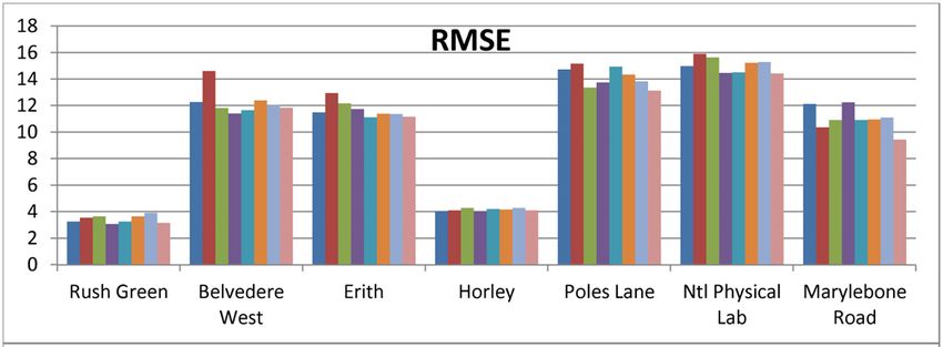
Figure 5 (a), (b) and (c) show the results for RMSE, MAPE (c) Heatmap of band accuracy.
and band accuracy, respectively, for the predicted AQI values.
It is clear that the results vary a lot across the different sensing
sites. This is because firstly, the different monitoring sites are achieving a band accuracy of close to 100% (over 99.6%, see
sited differently (e.g. kerbside vs. rural location) and located Fig. 5c). With respect to RMSE and MAPE, the proposed
in different kinds of areas which have different meteorologi- NARX methods perform the best on both approaches. It is
cal and pollution characteristics. Secondly, these sensing sites worth noting that even though the RMSE values do not show
measure different meteorological and pollution data, thus much difference between the evaluated machine learning
features of the model are different between different sites. algorithms, the MAPE values of LoR on both AQIPredict
Thirdly, pollutants’ concentrations are dispersed differently and Pollutant2AQI are much worse than the others. This is
and dominate different areas, depending upon on a number due to the fact that the AQI data values from Rush Green are
of factors such as industrial activities, vehicular emissions, small, hence, a small number of errors may not reflect much
human activities such as construction, etc. on the RMSE value but may show up in the MAPE which is
According to Table 2, Rush Green is a site recording six significantly affected when the calculation involves the ratio
kinds of meteorological data but only one type of pollu- of small actual values.
tion data: NO2 . Its AQI in Fig. 3 shows that the pollution Another similar sensing site is Horley, which records four
values range from 0 to around 100 and most of them are meteorological features and two pollutants’ data: NO2 and
below 25, i.e., the AQIs are always in the ‘Good’ band. For PM10 (with PM10 the dominant pollutant). The mean values
these reasons, all the methods perform well on this dataset of AQIs of this site are slightly higher than that of Rush Green,
VOLUME 6, 2018 78003Y. Zhou et al.: Data-Driven Air Quality Characterization for Urban Environments: A Case Study nevertheless, almost all the AQIs fall within the ‘Good’ band. AQIPredict NARX achieves the best RMSE, Pollutant2AQI Hence, the band accuracies of predicted values from this NARX achieves the best MAPE, while AQIPredict LoR site are also close to 100 percent (over 99.1%, see Fig. 5c). achieves the best band accuracy. RMSE and MAPE values are low for all the methods. RMSE To summarise, for RMSE, Pollutant2AQI NARX and values are close to each other as shown in Fig. 5a, but AQIPredict NARX perform the best on datasets from three the MAPE results of the Pollutant2AQI methods are less sites each, with AQIPredict LR showing the best performance than those of AQIPredict methods. Among them, the pro- on the seventh case. For MAPE values (see Fig. 5b), Pol- posed Pollutant2AQI NARX method performs the best for lutant2AQI NARX performs the best on datasets from four both evaluations. For band accuracy, Pollutant2AQI NARX sites, AQIPredict NARX performs the best on two, and Pollu- reaches an accuracy of 99.13%, slightly less than the best tant2AQI SVR performs the best on one. It is a mixed picture achieved result of 99.42% obtained by Pollutant2AQI LR and for band accuracy as shown in Fig. 5c, with Pollutant2AQI Pollutant2AQI LoR. NARX showing the best performance for three datasets, Belvedere West is a site with four meteorological features AQIPredict LR, AQIPredict LoR, and Pollutant2AQI SVR and four kinds of pollution data: NO2 , PM10 , O3 (dominant separately showing the best performance on one dataset each, pollutant), and PM2.5 . AQIs of this site ranges from 0 to and Pollutant2AQI LR and Pollutant2AQI LoR tied in for around 250, covering five bands. Most of the AQIs are located similar accuracies on the last one. Taking into account all the in the Good and Moderate bands. With regards to the evalu- datasets from the seven sites, Pollutant2AQI NARX performs ation results for this site, Pollutant2AQI NARX performs the the best on most of the datasets, and provides competitive best for all three metrics. results for the rest. This indicates that Pollutant2AQI NARX The Erith sensing site monitors three meteorological fea- has robust performance for different kinds of datasets and can tures and three kinds of pollutants: NO2 , PM10 (dominant), be recommended for AQI prediction. and PM2.5 . The AQIs of this site range from 0 to around 170, covering four bands, with the majority of the AQI values falling within the Good and Moderate bands. The AQIPredict LR method performs the best for RMSE (Fig. 5a) and band accuracy (Fig. 5c), while the Pollutant2AQI SVR performs the best for MAPE (Fig. 5b). Overall, the Pollutant2AQI methods have higher RMSE values but lower MAPEs. This shows that Pollutant2AQI methods can perform accurate pre- dictions when the actual values are small; however, for points where actual values are large, the predicted values of Pol- lutant2AQI methods are further from the actual values than those of other methods, which results in large RMSE values but still small MAPE values. Poles Lane and Ntl Physical Lab are two similar sites, which monitor the same three meteorological features and two kinds of pollution data: NO2 and O3 (dominant). Boxplot figures in Figure 3 show that their AQIs’ distributions are also similar. Compared to the other sites, RMSEs of these two sites are larger, band accuracies are smaller, but MAPEs do not show much difference. An interesting finding is that AQIPredict NARX performs the best for the RMSE and MAPE evaluations for both sites, but Pollutant2AQI NARX has a better band accuracy than AQIPredict NARX. For Poles Lane, Pollutant2AQI NARX achieves the best band accuracy, while for Ntl Physical Lab, band accuracy is about 5% lower than those of Poles Lane, and Pollutant2AQI SVR achieves the best band accuracy. FIGURE 6. Results of pollution data prediction of different learning The Marylebone Road kerbside site measures three algorithms. meteorological features and five kinds of pollution data: NO2 (dominant), PM10 , O3 , CO and SO2 . The majority of B. POLLUTANT PREDICTION: RESULT AND DISCUSSION the AQI values of this site are close to 50, which is the In addition to AQI prediction, we also compared MAPEs boundary between the Good and Moderate band. However, for the prediction of the individual pollutant values (as part the maximum AQI values reach the Hazardous band, i.e., the of the Pollutant2AQI approach) by the different methods, values cover the entire range of the 6 AQI bands; from Good i.e., LR, LoR, SVR, and NARX. The results are presented to Hazardous. For the prediction performance for this site, in Figure 6. We get the worst performance with LoR as 78004 VOLUME 6, 2018
Y. Zhou et al.: Data-Driven Air Quality Characterization for Urban Environments: A Case Study

the training algorithm across most of the datasets, with the                        REFERENCES
only exception being the MAPE results for PM10 data from                            [1] M. Finch. (2015). Urban Migration. [Online]. Available: www.uk.fujitsu.
Horley and the CO data from Marylebone Road (second low-                                com/innovation/megatrends
                                                                                    [2] J. Y. Zhu, C. Sun, and V. O. K. Li, ‘‘An extended spatio-temporal Granger
est MAPE value). For NO2 , the proposed NARX approach                                   causality model for air quality estimation with heterogeneous urban big
performs the best for 6 sites, while SVR performs the best                              data,’’ IEEE Trans. Big Data, vol. 3, no. 3, pp. 307–319, Sep. 2017.
on data from Belvedere West. Both SVR and NARX get the                              [3] BBC. (2018). Pollution Hotspots Revealed: Check Your Area. [Online].
                                                                                        Available: https://www.bbc.co.uk/news/science-environment-42566393
same MAPE on NO2 data from Marylebone Road. However,                                [4] C. P. Goeminne et al., ‘‘The impact of acute air pollution fluctuations on
the NARX method does not appear to be the best one for                                  bronchiectasis pulmonary exacerbation. A case-crossover analysis,’’ Eur.
predicting PM10 data. Among the four sites monitoring PM10                              Respiratory J., vol. 52, no. 1, Jul. 2018, Art. no. 1702557.
                                                                                    [5] DEFRA. (2018). UK AIR—Air Information Resource. [Online]. Available:
concentrations, LR achieves the two best MAPEs, while LoR                               https://uk-air.defra.gov.uk
and SVR achieving the best MAPE values on one dataset                               [6] Z. Qi, T. Wang, G. Song, W. Hu, X. Li, and Z. Zhang, ‘‘Deep air learning:
each. For O3 data, NARX performs the best for two datasets,                             Interpolation, prediction, and feature analysis of fine-grained air quality,’’
                                                                                        IEEE Trans. Knowl. Data Eng., vol. 30, no. 12, pp. 2285–2297, Dec. 2018.
with LR and SVR performing well on one each. SVR also                               [7] J. Garcia, J. Colosio, and P. Jamet, ‘‘Air quality indexes,’’ in Proc. 16th
performs the best on one PM2.5 dataset with NARX performs                               Conf. Environ. Commun. Inf. Soc., 2002, p. 112.
the best on the other one. NARX performs well for both SO2                          [8] Y. Zheng, F. Liu, and H.-P. Hsieh, ‘‘U-Air: When urban air quality infer-
                                                                                        ence meets big data,’’ in Proc. 19th ACM SIGKDD Int. Conf. Knowl.
and CO datasets.                                                                        Discovery Data Mining, Chicago, IL, USA, 2013, pp. 1436–1444.
   Overall, NARX can achieve a good performance for pre-                            [9] Y. Zheng, L. Capra, O. Wolfson, and H. Yang, ‘‘Urban computing: Con-
diction of pollution data except for that of PM10 . Therefore,                          cepts, methodologies, and applications,’’ ACM Trans. Intell. Syst. Technol.,
                                                                                        vol. 5, no. 3, pp. 1–55, 2014.
for predicting AQIs, NARX can be used on areas whose dom-                          [10] S. De, Y. Zhou, I. L. Abad, and K. Moessner, ‘‘Cyber–physical–social
inant pollutant is not PM10 , with LR proving to be a better                            frameworks for urban big data systems: A survey,’’ Appl. Sci., vol. 7, no. 10,
choice for such locations. This is in agreement with findings                           p. 1017, 2017.
                                                                                   [11] Y. Zhou, S. De, W. Wang, R. Wang, and K. Moessner, ‘‘Missing data
in [16], where multiple linear regression models achieved                               estimation in mobile sensing environments,’’ IEEE Access, vol. 6, no. 1,
better results than ANN for mean relative and absolute error                            pp. 69869–69882, Dec. 2018, doi: 10.1109/ACCESS.2018.2877847.
percentages as well as for RMSE for PM10 concentration                             [12] K. Hu, V. Sivaraman, H. Bhrugubanda, S. Kang, and A. Rahman, ‘‘SVR
                                                                                        based dense air pollution estimation model using static and wireless sensor
predictions.                                                                            network,’’ in Proc. IEEE SENSORS, Oct./Nov. 2016, pp. 1–3.
                                                                                   [13] K. Hu, A. Rahman, H. Bhrugubanda, and V. Sivaraman, ‘‘HazeEst:
VI. CONCLUSIONS AND NEXT STEPS                                                          Machine learning based metropolitan air pollution estimation from fixed
                                                                                        and mobile sensors,’’ IEEE Sensors J., vol. 17, no. 11, pp. 3517–3525,
In this paper we propose two approaches for AQI estimation                              Jun. 2017.
and prediction, both based on meteorological and historical                        [14] X. Yi, J. Zhang, Z. Wang, T. Li, and Y. Zheng, ‘‘Deep distributed fusion
pollutant data; one learns a model based on the previous AQI                            network for air quality prediction,’’ in Proc. 24th ACM SIGKDD Int. Conf.
                                                                                        Knowl. Discovery, Data Mining, London, U.K., 2018, pp. 965–973.
and meteorological data to predict AQIs, the other learns                          [15] K. P. Moustris, I. C. Ziomas, and A. G. Paliatsos, ‘‘3-day-ahead forecasting
models based on the previous pollution data and meteoro-                                of regional pollution index for the pollutants NO2 , CO, SO2 , and O3
logical data to predict pollution concentrations first and then                         using artificial neural networks in Athens, Greece,’’ Water, Air, Soil Pollut.,
                                                                                        vol. 209, no. 1, pp. 29–43, Jun. 2010.
compute AQIs. Both approaches can get good band accuracy                           [16] M. Cai, Y. Yin, and M. Xie, ‘‘Prediction of hourly air pollutant concentra-
(over 75%), as shown on the evaluations conducted across                                tions near urban arterials using artificial neural network approach,’’ Transp.
various datasets. The best approach is the latter approach                              Res. D, Transport Environ., vol. 14, no. 1, pp. 32–41, 2009.
                                                                                   [17] I. Juhos, L. Makra, and B. Tóth, ‘‘Forecasting of traffic origin NO and
combined with neural network, which achieves the lowest                                 NO2 concentrations by support vector machines and neural networks using
RMSE and MAPE across most of the evaluated datasets. This                               principal component analysis,’’ Simul. Model. Pract. Theory, vol. 16, no. 9,
approach gets very good band accuracies (more than 81%)                                 pp. 1488–1502, 2008.
                                                                                   [18] Y. Zheng et al., ‘‘Forecasting fine-grained air quality based on big data,’’
on all the datasets. However, by further analyzing the indi-                            in Proc. 21th ACM SIGKDD Int. Conf. Knowl. Discovery Data Mining,
vidual pollutant value prediction step, we found that a neu-                            Sydney, NSW, Australia, 2015, pp. 2267–2276.
ral network-based method is not the optimum at predicting                          [19] W. Wang, S. De, Y. Zhou, X. Huang, and K. Moessner, ‘‘Distributed sensor
                                                                                        data computing in smart city applications,’’ in Proc. IEEE 18th Int. Symp.
PM10 data. Therefore, we recommend using linear regression                              World Wireless, Mobile Multimedia Netw. (WoWMoM), Jun. 2017, pp. 1–5.
to predict AQI if the dominant pollution is PM10 in the                            [20] M. Sharma, S. Aggarwal, P. Bose, and A. Deshpande, ‘‘Meteorology-based
area of interest. In summary, the results show the feasibility                          forecasting of air quality index using neural network,’’ in Proc. IEEE Int.
                                                                                        Conf. Ind. Inform. (INDIN), Aug. 2003, pp. 374–378.
of our proposed approaches for predicting AQIs based on                            [21] K. Karatzas, A. Bassoukos, D. Voukantsis, F. Tzima, K. Nikolaou, and
meteorological data and the historical pollutant data/AQIs.                             S. Karathanasis, ‘‘ICT technologies and computational intelligence meth-
   In the future, we plan to analyze correlations between                               ods for the creation of an early warning air pollution information sys-
                                                                                        tem,’’ in Proc. Int. Conf. EnviroInfo (Environ. Inform. Ind. Ecol.), Aachen,
sensing sites located close to each other to uncover latent                             Germany, 2008, pp. 482–489.
similarities in pollutant or AQI patterns and to analyze if they                   [22] Y. Zhang, M. Bocquet, V. Mallet, C. Seigneur, and A. Baklanov, ‘‘Real-
are influenced by other environment factors such as green                               time air quality forecasting, part I: History, techniques, and current status,’’
                                                                                        Atmos. Environ., vol. 60, pp. 632–655, Dec. 2012.
cover or traffic. We also plan to further extend the analysis                      [23] Y. Ding, Y. Li, K. Deng, H. Tan, M. Yuan, and L. M. Ni, ‘‘Detecting and
of impact on air quality from different types of sensing areas                          analyzing urban regions with high impact of weather change on transport,’’
across different cities. Another future work is to infer the                            IEEE Trans. Big Data, vol. 3, no. 2, pp. 126–139, Jun. 2017.
                                                                                   [24] X. Lu, K. Ota, M. Dong, C. Yu, and H. Jin, ‘‘Predicting transportation
latent diurnal and seasonal pollution data patterns in different                        carbon emission with urban big data,’’ IEEE Trans. Sustain. Comput.,
parts of a city according to its built environment.                                     vol. 2, no. 4, pp. 333–344, Oct./Dec. 2017.

VOLUME 6, 2018                                                                                                                                                  78005
Y. Zhou et al.: Data-Driven Air Quality Characterization for Urban Environments: A Case Study
[25] R. Hassan and M. Li, ‘‘Urban air pollution forecasting using artificial GIDEON EWA received the B.Eng. degree in
intelligence-based tools,’’ in Air Pollution, V. Villanyi, Ed. Rijeka, Croatia: computer engineering from the University of Uyo,
IntechOpen, 2010. Nigeria, and the M.Sc. degree in mobile and satel-
[26] T. Ricardo-Aea et al., ‘‘Air pollution in the UK 2013,’’ lite communication from the University of Surrey,
Dept. Environ., Food Rural Affairs, Tech. Rep., Sep. 2014, pp. 1–81. U.K., in 2016. He is currently a Satellite System
[Online]. Available: https://uk-air.defra.gov.uk/assets/documents/reports/ Engineer with the Center for Satellite Technology
cat05/1409261329_air_pollution_uk_2013_issue_1.pdf Development, a research center under the National
[27] AirNow.gov. (May 2016). Technical Assistance Document for the Report-
Space Research and Development Agency, Abuja,
ing of Daily Air Quality—The Air Quality Index (AQI). Accessed:
Nigeria. His research interests are in wireless com-
Oct. 29, 2018. [Online]. Available: https://airnowtest.epa.gov/sites/default/
files/2018-05/aqi-technical-assistance-document-may2016.pdf munications, Internet of Things, smart cities, and
[28] T. Lin, B. G. Horne, P. Tiňo, and C. L. Giles, ‘‘Learning long-term machine learning.
dependencies in NARX recurrent neural networks,’’ IEEE Trans. Neural
Netw., vol. 7, no. 6, pp. 1329–1338, Nov. 1996.
[29] H. T. Siegelmann, B. G. Horne, and C. L. Giles, ‘‘Computational capa-
bilities of recurrent NARX neural networks,’’ IEEE Trans. Syst., Man,
Cybern. B, Cybern., vol. 27, no. 2, pp. 208–215, Apr. 1997.
[30] M. T. Hagan and M. B. Menhaj, ‘‘Training feedforward networks with
the Marquardt algorithm,’’ IEEE Trans. Neural Netw., vol. 5, no. 6,
pp. 989–993, Nov. 1994.
[31] R. Battiti, ‘‘1st-order and 2nd-order methods for learning—Between
steepest descent and Newton method,’’ Neural Comput., vol. 4, no. 2,
pp. 141–166, Mar. 1992. CHARITH PERERA (M’14) received the B.Sc.
[32] J. Neter, M. H. Kutner, C. J. Nachtsheim, and W. Wasserman, Applied degree (Hons.) in computer science from Stafford-
Linear Statistical Models, vol. 4. Homewood, IL, USA: Irwin, 1996. shire University, U.K., the MBA degree in busi-
[33] D. W. Hosmer, Jr., S. Lemeshow, and R. X. Sturdivant, Applied Logistic ness administration from the University of Wales,
Regression, vol. 398. Hoboken, NJ, USA: Wiley, 2013. Cardiff, U.K., and the Ph.D. degree in computer
[34] A. J. Smola and B. Schölkopf, ‘‘A tutorial on support vector regression,’’ science from The Australian National University,
Statist. Comput., vol. 14, no. 3, pp. 199–222, Aug. 2004.
Canberra, Australia. He was with the Informa-
[35] H. Drucker, C. J. Burges, L. Kaufman, A. Smola, and V. Vapnik, ‘‘Support
tion Engineering Laboratory, ICT Centre, CSIRO.
vector regression machines,’’ in Proc. Adv. Neural Inf. Process. Syst., vol. 9,
1997, pp. 155–161. He is currently a Lecturer (Assistant Professor)
with Cardiff University, U.K. His research inter-
ests are Internet of Things, sensing as a service, privacy, middleware plat-
YUCHAO ZHOU received the B.S. degree in forms, and sensing infrastructure. He is a member of ACM.
telecommunications engineering with manage-
ment from a joint program between the Bei-
jing University of Posts and Telecommunications,
China, and the Queen Mary University of London,
U.K., in 2011, and the M.Sc. degree in commu-
nications networks and software and the Ph.D.
degree in electronic engineering from the Univer-
sity of Surrey, Guildford, U.K., in 2012 and 2018,
respectively. He is currently a Research Fellow
with the Institute for Communication Systems, University of Surrey. His
research interests include semantic Web, search techniques for the Web of
Things, and Internet of Things applications in smart cities.
KLAUS MOESSNER (M’97–SM’13) was involved
in the definition and evaluation of cooperation
SUPARNA DE (M’14) received the M.Sc. and management between autonomous entities and in
Ph.D. degrees in electronic engineering from the the UniverSelf Project. He was a Technical Man-
University of Surrey in 2005 and 2009, respec- ager of the iCore Project and the H2020 Project
tively. She is currently a Senior Research Fellow CPaaS.io. He was a Project Leader of IoT.est and
with the Institute for Communication Systems, SocIoTal. He is currently a Professor with the
University of Surrey. She leads technical work Institute for Communication Systems, University
areas related to various aspects of service provi- of Surrey. He currently leads the iKaaS Project and
sioning and data analysis in the Internet of Things Working Area 6 with the System Architecture in
domain in several EU projects such as TagItSmart, the 5G Innovation Centre, University of Surrey. His research interests include
iKaaS, IoT.est, iCore, and IoT-A. Her research cognitive networks, knowledge generation, and reconfiguration and resource
has been supported by grants from the EC H2020 and FP7 programs and management. He was the Founding Chair of the IEEE DYSPAN Working
through DTI, U.K.-funded programs. Her current research interests include Group (WG6) on sensing interfaces for future and cognitive communication
knowledge engineering methods, machine learning for data analytics, Web systems.
of Things, and semantic association analysis. She is a member of ACM.
78006 VOLUME 6, 2018You can also read