Decadal Oscillation in the Predictability of Palmer Drought Severity Index in California - MDPI
←
→
Page content transcription
If your browser does not render page correctly, please read the page content below
climate
Article
Decadal Oscillation in the Predictability of Palmer
Drought Severity Index in California
Nazzareno Diodato 1 , Lelys Bravo de Guenni 2 , Mariangel Garcia 3          and Gianni Bellocchi 1,4, *
 1    Met European Research Observatory, 82100 Benevento, Italy; scodalabdiodato@gmail.com
 2    Division of Statistics, Northern Illinois University, DeKalb, IL 60115, USA; lelysbravo@gmail.com
 3    Computational Science Research Center, San Diego State University, San Diego, CA 92182-7720, USA;
      mvgarcia@sdsu.edu
 4    UCA, INRA, VetAgro Sup, Unité Mixte de Recherche sur Écosystème Prairial (UREP),
      63000 Clermont-Ferrand, France
 *    Correspondence: gianni.bellocchi@inra.fr; Tel.: +33-4-4376-1601

 Received: 23 November 2018; Accepted: 1 January 2019; Published: 3 January 2019

 Abstract: Severity of drought in California (U.S.) varies from year-to-year and is highly influenced
 by precipitation in winter months, causing billion-dollar events in single drought years. Improved
 understanding of the variability of drought on decadal and longer timescales is essential to support
 regional water resources planning and management. This paper presents a soft-computing approach
 to forecast the Palmer Drought Severity Index (PDSI) in California. A time-series of yearly data
 covering more than two centuries (1801–2014) was used for the design of ensemble projections to
 understand and quantify the uncertainty associated with interannual-to-interdecadal predictability.
 With a predictable structure elaborated by exponential smoothing, the projections indicate for the
 horizon 2015–2054 a weak increase of drought, followed by almost the same pace as in previous
 decades, presenting remarkable wavelike variations with durations of more than one year. Results
 were compared with a linear transfer function model approach where Pacific Decadal Oscillation and
 El Niño Southern Oscillation indices were both used as input time series. The forecasted pattern shows
 that variations attributed to such internal climate modes may not provide more reliable predictions
 than the one provided by purely internal variability of drought persistence cycles, as present in the
 PDSI time series.

 Keywords: drought; ensemble forecast; exponential smoothing; transfer function modelling

1. Introduction
     Drought is a fundamental feature of the climate of North America, where several regions of
western United States (U.S.) have experienced protracted decadal-scale dry periods in the past
centuries [1] Hydrologic droughts in western U.S. were already widespread and persistent during the
so-called Medieval Climatic Anomaly, roughly in the period 900–1300 AD [2], with mega-drought
in southern California during 832–1074 AD and 1122–1299 AD [3,4]. Multi-year droughts have also
recurred in more recent times, e.g., in 1818–1824, 1827–1829, 1841–1848 and 1855–1865 (Figure 1),
causing tremendous disruption on social, agricultural, ecological and economic fronts [5]. Five major
droughts followed, which ended in 1924, 1935, 1950, 1960 and 1977. As well, the one started in 2012 [1]
resulted in statewide proclamations of emergency [6]. Much of the water supply for California is
derived from the Sacramento-San Joaquin River Delta (located in Northern California) via pumps
located at the southern end of the delta. However, in recent times, California’s water resources
have been subject to increased stress from a combination of factors including a growing population,
groundwater deficit, limitations on extraction of water for the protection of fish, and increased

Climate 2019, 7, 6; doi:10.3390/cli7010006                                     www.mdpi.com/journal/climate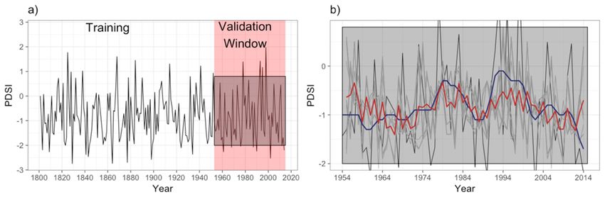
Climate 2019, 7, 6 2 of 17
competition
Climate 2018,for
6, x available water [6]. Over 2012–2016, drought conditions impacted surface2 of
FOR PEER REVIEW water
18
supplies, and increased agricultural demand and land subsidence owing to groundwater extraction.
supplies,
These factorsand increased
inspired agricultural demand
the development and land
of legislation subsidence
to regulate owing to groundwater
groundwater resources and extraction.
financially
Thesesustainable
support factors inspired the development
groundwater management of as
legislation to regulate
well as cleanup groundwater
and storage resources
[7]. Water and
management
financially
in the state (whichsupporthassustainable
been studiedgroundwater
extensivelymanagement
[8]) showsasthat
wellthe
as California
cleanup andcasestorage [7]. Water of
is exemplary
the management
preparednessinand the state (which
response has beenrequired
measures studied extensively
to cope with [8])extreme
shows that the California
drought case is to
events, adapt
exemplary of the preparedness and response measures required to cope with extreme drought
them and build long-term resilience [9]. How drought may change in future is of great concern as
events, adapt to them and build long-term resilience [9]. How drought may change in future is of
global warming continues [10]. Yet, how has an extreme drought occurrence over California shifted as
great concern as global warming continues [10]. Yet, how has an extreme drought occurrence over
a result of the change in climate since historical times? How can we see droughts coming? If we are
California shifted as a result of the change in climate since historical times? How can we see droughts
dry during one drought year, will we likely be dry for other drought years, and then for a decade or
coming? If we are dry during one drought year, will we likely be dry for other drought years, and
more?
thenHow
for acyclical
decadewill these patterns
or more? be and
How cyclical how
will arepatterns
these they predictable
be and how overare
multidecadal time-scales?
they predictable over
To answer
multidecadal time-scales? To answer these questions, we examined (with focus on California)the
these questions, we examined (with focus on California) uncertainties in estimating
future ramifications
uncertainties of years ofthe
in estimating drought, and how drought
future ramifications changes
of years may recur
of drought, in thedrought
and how near future using
changes
the may
Palmer Drought
recur Severity
in the near futureIndex
using(PDSI).
the Palmer Drought Severity Index (PDSI).
Figure 1. Mapped
Figure patterns
1. Mapped patternsofofreconstructed
reconstructedPDSI
PDSI for
for some intervalsin
some intervals in19th
19thcentury
centuryacross
across
thethe U.S.
U.S.
(modified from
(modified Cole
from et al.
Cole [5]).
et al. [5]).
ManyMany of ofdrought
drought indices
indicesdeveloped
developed for for thethe purpose
purpose of drought
drought monitoring
monitoringare arebased
basedonon
meteorological
meteorological andand hydrological
hydrological variables,
variables,whichwhichshow show thethe size, duration,
duration,severity
severityandandspatial
spatial extent
extent
of droughts.
of droughts. The The PalmerDrought
Palmer DroughtSeverity
Severity Index
Index(PDSI)(PDSI)isissuch
suchananexample.
example. Originally developed
Originally developedby
Palmer
by Palmer [11], it is one of the most well-known and widely used drought indices
it is one of the most well-known and widely used drought indices in the U.S. [12,13] in the U.S. [12,13] and
andbeyond
beyond[14–17]
[14–17] PDSI
PDSI values are are
values computed
computed alongalongthe soil
themoisture balancebalance
soil moisture that requires time series
that requires time
of of
series temperature,
temperature, precipitation,
precipitation, ground moisture
ground moisturecontent (or available
content water-holding
(or available capacity)
water-holding and
capacity)
andpotential
potentialevapotranspiration.
evapotranspiration. TheThe
calculation
calculation algorithm
algorithmof PDSI—either
of PDSI—either in itsinoriginal version
its original by
version
Palmer [11] or in modified ones [18] is thus a reflection of how much
by Palmer [11] or in modified ones [18] is thus a reflection of how much soil moisture is currently soil moisture is currently
available compared to that for normal or average conditions. The PDSI incorporates both
available compared to that for normal or average conditions. The PDSI incorporates both precipitation
precipitation and temperature data in a simplified, though reasonably realistic, water balance model
and temperature data in a simplified, though reasonably realistic, water balance model that accounts
that accounts for both supply (rain or snowfall water equivalent) and demand (temperature,
for both supply (rain or snowfall water equivalent) and demand (temperature, transformed into
transformed into units of water lost through evapotranspiration), which affect the content of a two-
units of water lost through evapotranspiration), which affect the content of a two-layer soil moisture
layer soil moisture reservoir model (a runoff term is also activated when the reservoir is full). Not
reservoir model
explicitly (a runoff
bounded, term typically
the PDSI is also activated
falls in the whenrangethe reservoir
from is full).
−4 (extreme Not explicitly
drought) bounded,
to +4 (extremely
the wet).
PDSI Thetypically
PDSI is falls in the range from
a dimensionless quantity−4 (extreme
for comparisondrought) to +4
across (extremely
regions wet). The
with radically PDSI is
different
a dimensionless quantity for comparison across regions with radically different
precipitation regimes. This means that there are limitations in the use of this index at specific scales, precipitation regimes.
Thisfor
means
which that there
other are limitations
drought in the
indices have beenusedeveloped
of this index at specific scales,
to characterize for which other
local agricultural and drought
socio-
indices have been
economic contextsdeveloped
[19]. to characterize local agricultural and socio-economic contexts [19].
Land-atmosphere
Land-atmosphereinteractionsinteractions cancan introduce
introduce persistence
persistence into into droughts
droughts because
becausereduced
reduced
precipitation
precipitation lowers
lowers soilsoil moisture,reduces
moisture, reducessurfacesurface evapotranspiration
evapotranspiration and, and,with
withless
lessvapor
vapor in in
thethe
atmosphere, further reduces
atmosphere, further reduces precipitation. precipitation. In this sequence, soil moisture adjustment
this sequence, soil moisture adjustment occurs with occurs with a
lengthofoftime,
a length time,whichwhich introduces
introduces aa laglag and
andaamemory.memory.Depending
Depending onon situations, there
situations, might
there be abe
might
strong coupling between soil moisture and precipitation, and land
a strong coupling between soil moisture and precipitation, and land surface processes can lead surface processes can lead to to
persistence [20]. The calculation of PDSI is intended to model soil moisture
persistence [20]. The calculation of PDSI is intended to model soil moisture persistence (or memory). persistence (or memory).
The combination of past wet/dry conditions with past PDSI data means that the PDSI for a given time
Climate 2019, 7, 6                                                                                3 of 17

The combination of past wet/dry conditions with past PDSI data means that the PDSI for a given
time step (generally one month) can be seen as a weighed function of current moisture conditions
and a contribution of PDSI over previous times [21]. In the light of this persistence structure, PDSI
chronologies can be used to reconstruct drought conditions, but persistence can also be a criterion to
be used as a measure of predictability [16].
     This paper deals with time series analysis (TSA) related to PDSI dynamics. Several statistical
TSA approaches were applied to predict climate variables, including their extremes [22,23]. Mossad
and Alazba [24] proved the potential ability of these modelling approaches to forecast drought.
However, drought forecasts performed at monthly time-scale for early warning [25–29] do not
account for long-term patterns of evolution, which are essential to study and monitor drought
from a climate perspective [30]. Here, we target annual to decadal time scales. We investigate
to what extent TSA model simulations may provide reliable forecasts of future hydrological
changes. Although research on meteorological drought (that is, when dry weather patterns
dominate) is particularly difficult because of the complex and heterogeneous character of drought
processes, their temporal trends respond to climate fluctuations (e.g., large-scale atmospheric
circulations). Specifically, the work explores a homogenized long series of annual PDSI data (1801–2014)
as derived for California by Griffin and Anchukaitis [1] and accessible at https://www1.ncdc.
noaa.gov/pub/data/paleo/treering/reconstructions/california/griffin2015drought.txt (identifier
‘precip-ONDJFMAMJ-rec-2rmse’, providing precipitation anomalies serving as reasonable proxy
of PDSI data taken at the lower limit of twice the root mean square error). Then the study assesses the
response of an exponential smoothing (ES) model, using an ensemble prediction approach. ES [31,32]
and autoregressive integrated moving average (ARIMA) models [33] are the most representative
methods in TSA. In this study, ES was used because it is known to be optimal for a broader class
of state-space models than ARIMA models [32]. ES responds easily to changes in the pattern of
time series [34] and is often referred to as a reference model for time-pattern propagation into the
future [35,36]. It is also less complex in its formulation and, as such, it was expected to be easier in
identifying the causes of unexpected results. The ensemble approach has been adopted as a way to
consider uncertainty in hydrological forecasting, and thus enhance accuracy by combining forecasts
made at different lead times, as in Armstrong [37] and in previous authors’ papers [38–41]. A lengthy
PDSI series offers a unique opportunity to explore past interannual-to-interdecadal climate variability,
under the assumption that the past interannual climate variability, with its internal dependence
structure, can be used to replicate future PDSI ramifications at the local scale. This approach was
compared with the more traditional TSA approach using transfer function models (TFM), introduced
by Box and Jenkins [42] and re-visited by Shumway and Stoffer [43]. In this case, input time series of
El Niño Southern Oscillation (ENSO) and the Pacific Decadal Oscillation (PDO) were considered as
impulse inputs to the output PDSI time series. An approximate ensemble approach was also developed
under the transfer function models (TFM) framework for comparison purposes with the ES results.
For California, there are now accessible accurate long-time series of PDSI. Our focus is motivated
because severe and widespread drought are of particular concern for this U.S. state [44].

2. Materials and Methods

2.1. Environmental Setting and Data
     The California’s climate varies widely, from hot desert to subarctic, depending on latitude,
elevation, and proximity to the coast. California’s coastal regions, the Sierra Nevada foothills, and
much of the Central Valley have a Mediterranean climate, with warm to hot, dry summers, and mild,
moderately wet winters (Figure 2a,b). The influence of the ocean generally moderates temperature
extremes, creating warmer winters and substantially cooler summers in coastal areas. The rainy period
in most of the country is from November to April (Figure 2a). Prevailing westerly winds from the
Pacific Ocean also bring moisture. The average annual rainfall in California is about 350 mm, with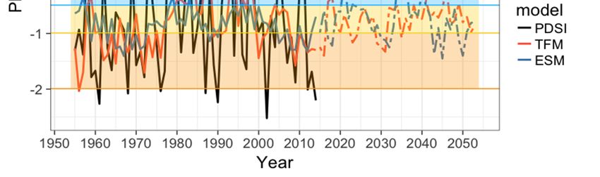
Climate 2019, 7, 6 4 of 17
the northern parts of the state generally receiving higher rain amounts than the south. The reference
Climate 2018, 6, x FOR PEER REVIEW 4 of 18
evapotranspiration follows a more complex pattern, mostly in relation to elevation and distance from
sea (Figure 2c). Temperature and evapotranspiration are especially important in California, where
sea (Figure 2c). Temperature and evapotranspiration are especially important in California, where
water storage
water storageand distribution
and distributionsystems
systemsare
arecritically
critically dependent on winter/spring
dependent on winter/spring rainfall,
rainfall, andand excess
excess
water demand is typically met by groundwater withdrawal [45]. The PDSI time series
water demand is typically met by groundwater withdrawal [45]. The PDSI time series derived from derived from
Griffin andand
Griffin Anchukaitis
Anchukaitis [1][1]reconstructed
reconstructeddrought
drought conditions for California.
conditions for California.
Figure 2. (a)
Figure Rainfall
2. (a) monthly
Rainfall monthlyregime
regimewith
withrelative bioclimaticpatterns
relative bioclimatic patternsfor
forCalifornia;
California;(b)(b) mean
mean annual
annual
smoothed
smoothed 20-km spatial
20-km precipitation
spatial overover
precipitation the period 1961–1990;
the period (c) the(c)
1961–1990; corresponding annualannual
the corresponding reference
evapotranspiration (arranged via (arranged
reference evapotranspiration LocClim FAOvia software,
LocClim http://www.fao.org/land-water/land/land-
FAO software, http://www.fao.org/land-
water/land/land-governance/land-resources-planning-toolbox/category/details/en/c/1032167).
governance/land-resources-planning-toolbox/category/details/en/c/1032167).
2.2.2.2.
Exponential Smoothing
Exponential Smoothing
TheTheexponential
exponential smoothing
smoothing(a(apopular
popular scheme
scheme to to produce
producesmoothedsmoothedtime time series)
series) is aisrelatively
a relatively
simple
simpleprototype
prototypemodel
modelfor forTSA-based
TSA-based forecasting, analysis and
forecasting, analysis and re-analysis
re-analysisofofenvironmental
environmental
variables
variables [46,47].
[46,47]. It It useshistorical
uses historicaltime
time series
series data under
under the theassumption
assumptionthat the
that thefuture
future will likely
will likely
resemble the past, in an attempt to identify specific patterns in the data, and
resemble the past, in an attempt to identify specific patterns in the data, and then project and extrapolate then project and
extrapolate
those patternsthose patterns
into the futureinto the future
(without (without
using the model usingto the model to
identify identify
the causestheof causes of patterns).
patterns). Compared
Compared
to other to other
techniques techniques
(e.g., moving(e.g., movingwhich
averages), averages),
equally whichweightequally
pastweight past observations,
observations, exponential
exponential
smoothing smoothingexponentially
apportions apportions exponentially
decreasing decreasing
weights as weights as observations
observations get older.
get older. This This
means
means that recent observations are given relatively more weight
that recent observations are given relatively more weight in forecasting than older observations. in forecasting than older
observations. To compute predictions based on the observed time series of PDSI data, we made use
To compute predictions based on the observed time series of PDSI data, we made use of available
of available knowledge concerning the period of the system under investigation [48]. The following
knowledge concerning the period of the system under investigation [48]. The following periodic
periodic simple exponential smoothing [35] was selected as reference model for time-pattern
simple exponential smoothing [35] was selected as reference model for time-pattern propagation into
propagation into the future:
the future:
F ((X ))tR+m = = α · · St (1) (1)
It− p
where ( ) represents the m-step-ahead forecast from the annual series of the variable X (PDSI)
where F ( X )tR+m represents the m-step-ahead forecast from the annual series of the variable X (PDSI) on
on N years for an ensemble of R runs; St is the smoothed PDSI at decadal scale centered on time-year
N years for an(2));
t (Equation ensemble
α is theof R runs; Sparameter
smoothing t is the smoothed PDSI
for the data; It−patisdecadal scale centered
the smoothed cycle index the end t
onattime-year
of period t, its number being defined by the periods p in the seasonal cycle (Equation (3))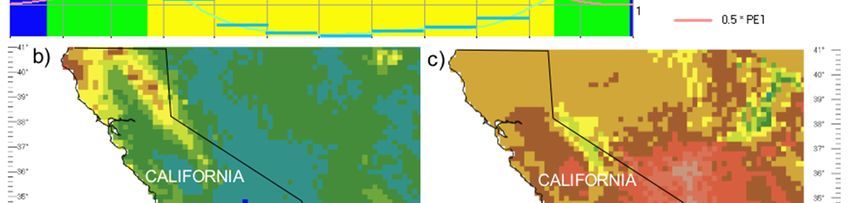
Climate 2019, 7, 6                                                                                   5 of 17

(Equation (2)); α is the smoothing parameter for the data; It−p is the smoothed cycle index at the end of
period t, its number being defined by the periods p in the seasonal cycle (Equation (3))

                                                      Xt
                                          St = α ·         + (1 − α)·St−1                               (2)
                                                     It− p

                                                      Xt
                                        It− p = δ·           + (1 − δ)· It−1                            (3)
                                                     S( X )t
where δ is smoothing parameter for cyclical indices.

2.3. Transfer Function Models
     Results from seasonal exponential smoothing (that uses the temporal dependence structure of the
time series itself to reproduce the time series behavior in the future) were compared to an alternative
methodology based on transfer function models (TFM). It represents a linear transfer function approach
where input time series potentially impacting the drought behavior at large spatial scales are used
as explanatory time series variables in a lagged regression model. The methodology called TFM
was introduced by Box and Jenkins [25] and re-visited by de Guenni et al. [49] and Shumway and
Stoffer [43] (2017) to forecast monthly rainfall in the coast of Ecuador based on El Niño indices and
model the impact of El Niño on fish recruitment, respectively.
     In a TFM, the output series (in this case PDSI) can be represented as:

                     Y (t) = α1 ( B)· X1 (t) + α2 ( B)· X2 (t) + . . . + αk ( B)· Xk (t) + η (t)        (4)

where X1 (t), X2 (t), . . . , Xk (t) are the input time series to be considered as explanatory variables
contributing to the temporal dynamics of the output series Y(t) and η(t) is a stationary random process.
The terms α1 (B), α2 (B), . . . , αk (B) are fractional polynomials in the back-shift operator B (such that
BS (X(t) = X(t − s)) of the form:

2.4. Model Validation Methods
      To ensure the optimal runs over the hold back prediction (testing validation), model
parameterization was achieved by minimizing together the Root Mean Squared Error (RMSE) and the
Mean Absolute Scaled Error (MASE), and maximizing the correlation coefficient (R). The commonly
used RMSE quantifies the differences between predicted and observed values, and thus indicates
how far the forecasts are from actual data. A few major outliers in the series can skew the RMSE
statistic substantially because the effect of each deviation on the RMSE is proportional to the size of
the squared error. The overall, non-dimensional measure of the accuracy of forecasts MASE [50] is
less sensitive to outliers than the RMSE. The MASE is recommended for determining comparative
accuracy of forecasts [51], because it examines the performance of forecasts relative to a benchmark
forecast. It is calculated as the average of the absolute value of the difference between the forecast
and the actual value divided by the scale determined by using a random walk model (naïve reference
model on the history prior to the period of data held back for model training). MASE < 1 indicates
that the forecast model is superior to a random walk. The correlation coefficient between estimates
and observations [52] (anti-correlation) (perfect correlation)—assesses linear relationships, in that
forecasted values may show a continuous increase or decrease as actual values increase or decrease.
Its extent is not consistently related to the accuracy of the estimates. WESSA R–JAVA web [53] was
used to assess model simulations with spreadsheet-based support.
      In order to quantify long-range dependence and appraise the cyclical-trend patterns in the series,
we estimated the Hurst [54] H exponent (rate of chaos), which is related to the fractal dimension
D = 2 − H of the series. Long memory occurs when 0.5 < H < 1.0, that is, events that are far apart are
correlated because correlations tend to decay very slowly. On the contrary, short-range dependence
0.0 < H < 0.5 is characterized by quickly decaying correlations, i.e., past trends tend to revert in the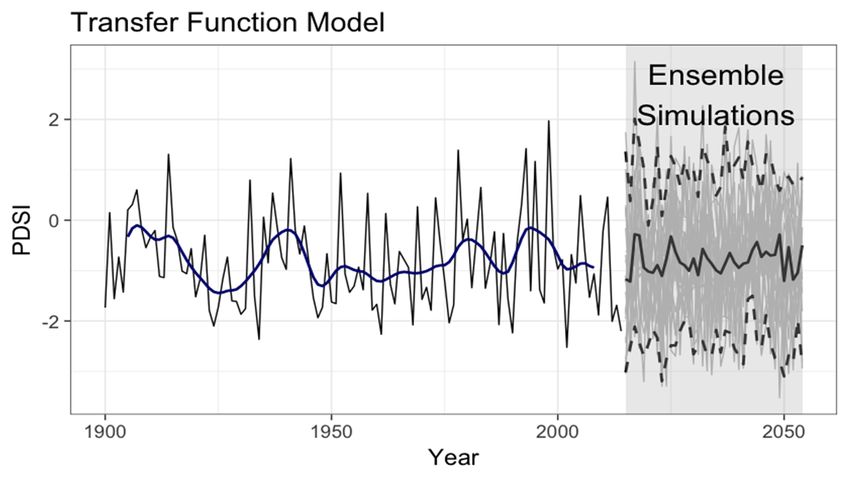
Climate 2019, 7, 6 6 of 17
future (an up value is more likely followed by a down value). Calculating the Hurst exponent is
not straightforward because it can only be estimated and several methods are available to estimate
it, which often produce conflicting estimates [55,56]. Using SELFIS (SELF-similarity analysis [55],
we referred to two methods, which are both credited to be good enough to estimate H [57]: the widely
used rescaled range analysis (R/S method) [58], and the ratio variance of residuals method, which is
known
Climateto2018,
be unbiased almost
6, x FOR PEER through all Hurst range [59]. Long-memory in the occurrence 6ofof PDSI
REVIEW 18
values was also analyzed to see if the memory characteristic is correlated with the length of the time
values was also analyzed to see if the memory characteristic is correlated with the length of the time
series. To determine whether this characteristic changes over time, the Hurst exponent was not only
series. To determine whether this characteristic changes over time, the Hurst exponent was not only
estimated for the full time series (1801–2014), but also for a shorter series starting in 1901 (the most
estimated for the full time series (1801–2014), but also for a shorter series starting in 1901 (the most
recent period, which is also the period held out of the calibration process).
recent period, which is also the period held out of the calibration process).
3. Results and Discussion
3. Results and Discussion
3.1. Data Analysis
3.1. Data Analysis
The first step in any time-series analysis and forecasting is to plot the observations against time,
The first step in any time-series analysis and forecasting is to plot the observations against time,
to gain an insight into possible trends and/or cycles associated with the temporal evolution of datasets.
to gain an insight into possible trends and/or cycles associated with the temporal evolution of
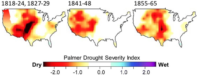
Figure 3a shows that the PDSI time series presents important inter-annual and decadal variability,
datasets. Figure 3a shows that the PDSI time series presents important inter-annual and decadal
with
variability, changes
smooth with smoothin its structure
changes in itsand turning
structure andpoints
turningwhich
pointshelp
whichinhelp
orienting the choice
in orienting of the
the choice
most
of the most appropriate forecasting method [60]. Two homogeneity tests indicate a stepwise shiftininthe
appropriate forecasting method [60]. Two homogeneity tests indicate a stepwise shift
observational seriesseries
the observational in theinyears justjust
the years before 1920.
before 1920.The
TheBuishand
Buishand range test[61]
range test [61]places
places
thethe change
change
point
point in 1969, whereas the Mann-Whitney-Pettitt test [62] locates it in 1920 but the two tests areare
in 1969, whereas the Mann-Whitney-Pettitt test [62] locates it in 1920 but the two tests notnot
significant (p > 0.10), from which the series can be considered as relatively stationary.
significant (p > 0.10), from which the series can be considered as relatively stationary.
Figure 3. (a)
Figure 3. Observed Palmer
(a) Observed Drought
Palmer Severity
Drought IndexIndex
Severity time-series (blue(blue
time-series curvecurve
1801–2014) with training
1801–2014) with
andtraining
validation periods; (b)
and validation for the
periods; (b)validation period,period,
for the validation the simulated series
the simulated (plume,
series light
(plume, grey)
light with
grey)
both theboth
with ensemble mean (red
the ensemble meancurve) and the
(red curve) observed
and Gaussian
the observed FilterFilter
Gaussian withwith
11-year smoothing
11-year smoothing(bold
grey curve).
(bold grey curve).
TheThe
smoothed
smoothedperiodogram
periodogram of of the
the PDSI
PDSI time series
series (Figure
(Figure4)4)was
wascalculated
calculated byby using
using thethe
smoothing method [63] implemented in the R software [64] This estimate shows
smoothing method [63] implemented in the R software [64] This estimate shows that most of the total that most of the total
variability
variability in in
thethe seriesis isassociated
series associatedwith
with both
both short
short and
and large
large frequencies.
frequencies.TheThemultiple
multipleobserved
observed
maxima
maxima in power
in the the power spectrum
spectrum confirm
confirm the complex
the complex interactions
interactions of several
of several physicalphysical drought-
drought-triggering
triggering
processes processes
acting acting
at several at several
time scales.time
The scales.
maximum The maximum
estimatedestimated spectraloccurs
spectral density densityatoccurs at
frequency
frequency 0.185, which corresponds to a cycle of 5.4 years [65]. This cycle might
0.185, which corresponds to a cycle of 5.4 years [65]. This cycle might be associated with El Niño be associated with El
Niño phenomenon,
phenomenon, but otherbut other frequencies
frequencies have alsohave also an important
an important contribution
contribution to the series
to the overall overallvariability.
series
variability.
3.2. Validation Results and PDSI Time Series Predictability
The whole of the PDSI time series (214 years of data from 1801 to 2014) was segregated into sub-
sets for the purposes of training and validation (Figure 3a). The choice of 1801 as starting time of the
series was driven by the necessity of having a sufficient amount of data for training without laying
too long back in time, considering that with at least 50 observations are necessary for performing
time-series analysis/modelling [66]. On the other hand, with at least 150–200 observations potentially
reliable forecasts can be obtained for 30 to 50 steps ahead [67]. Forecasts were performed for the 40-
year follow-up period (Figure 3b). Alternative initial conditions were simulated for each run, taking
periods with a different start year (in 10-year steps-up from year 1801 to 1900) and periodical cycles
(41, 42 and 43 years) for model training (training datasets).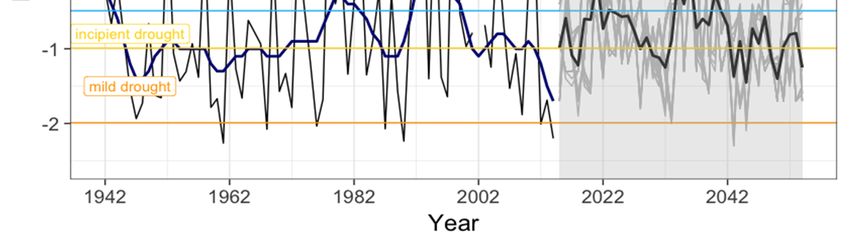
Climate 2019, 7, 6                                                                                                  7 of 17
   Climate 2018, 6, x FOR PEER REVIEW                                                                           7 of 18

      Figure 4. Smoothed
         Figure 4. Smoothed  periodogram
                              periodogramofofthethePDSI
                                                   PDSI time series(bandwidth
                                                        time series (bandwidthisisa ameasure
                                                                                      measureof of
                                                                                                thethe width
                                                                                                    width     of the
                                                                                                          of the
      frequency  interval
         frequency        used
                    interval usedininthe
                                       thesmoothing
                                           smoothingprocedure).
                                                     procedure).

3.2. Validation   Results and
         For 1954–2014         PDSI3b),
                           (Figure    Time
                                         theSeries Predictability
                                              simulation   results for validation testing are quite promising,
   judging
      The whole of the PDSI time series (214 years of (red
              by the closeness   of ensemble   prediction  mean   datacurve)  to theto
                                                                        from 1801    observed
                                                                                        2014) was 11-year Gaussianinto
                                                                                                      segregated
sub-sets for the purposes of training and validation (Figure 3a). The choice of 1801 as starting high
   Filter  (black curve)  PDSI  evolution.  The  results indicate that the ES model   performs    well at both time of
theand
    serieslow  frequency
             was  driven byvariability,   which
                              the necessity       is consistent
                                             of having            withamount
                                                         a sufficient   inter-annual
                                                                                of datatoforinter-decadal  climate-
                                                                                              training without  laying
   variability. In fact, the residuals between predicted and observed time-series are coherent in the
too long back in time, considering that with at least 50 observations are necessary for performing
   validation period: residual histograms and Q-Q plots do not identify substantial departures from
time-series analysis/modelling [66]. On the other hand, with at least 150–200 observations potentially
   normality in both the official run with the longest training time (Figure 5a,a1) and the average
reliable forecasts can be obtained for 30 to 50 steps ahead [67]. Forecasts were performed for the
   (ensemble mean) of all the runs (Figure 5b,b1).
40-year follow-up period (Figure 3b). Alternative initial conditions were simulated for each run, taking
         The data are somewhat right-skewed; however, the right tail of the distribution is fairly closely
periods    with a different
   approximated               start year
                     by the normal       (in 10-year
                                     distribution,     steps-up
                                                    with          from
                                                          some high      year 1801
                                                                     extreme        to 1900) and periodical cycles
                                                                               values.
(41, 42 and 43 years) for model training (training datasets).
      For 1954–2014 (Figure 3b), the simulation results for validation testing are quite promising,
judging by the closeness of ensemble prediction mean (red curve) to the observed 11-year Gaussian
Filter (black curve) PDSI evolution. The results indicate that the ES model performs well at both high
and low frequency variability, which is consistent with inter-annual to inter-decadal climate-variability.
In fact, the residuals between predicted and observed time-series are coherent in the validation period:
residual histograms and Q-Q plots do not identify substantial departures from normality in both the
official run with the longest training time (Figure 5a,a1) and the average (ensemble mean) of all the
runs (Figure 5b,b1).
      The data are somewhat right-skewed; however, the right tail of the distribution is fairly closely
approximated by the normal distribution, with some high extreme values.
      In the validation stage, RMSE and MASE were equal to 1.0 and 0.68, respectively, which indicate
a satisfactory performance, and that the forecast model is superior to a random walk. The estimated
Hurst (H) exponent values are reported in Table 1.

      Table 1. Estimated values of the Hurst (H) exponent (with two methods) for the PDSI annual series as
      a whole and for a reduced number of years.

     Hurst (H) Exponent/Estimation Method            Whole Series (1801–2014)         Reduced Series (1901–2014)
                Rescaled range (R/S)                             0.611                            0.743
              Ratio variance of residuals                        0.611                            0.550

     With the R/S method, the H was found to be greater than 0.6 in both the whole series (0.611) and
the sub-set 1901–2014 (0.743), which is around the threshold of 0.65 used by [68] to identify series than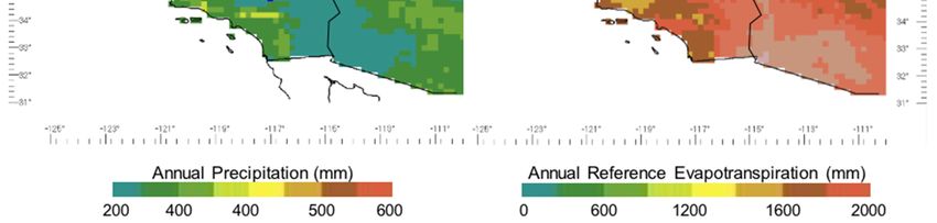
Climate 2019, 7, 6                                                                                                   8 of 17

can be predicted accurately. In the case of the variance of residuals method, we have a situation in
which obtained results are hard for interpretation. With an increase of the number of series terms
(amount of observations), the Hurst exponent is expected to get closer to 0 [69], i.e., the memory effect
decreases. However, with the variance residuals method, the estimated Hurst exponent moves away
from 0.5 with the whole of the time series (0.611 against 0.550 with the sub-set 1901–2014). These
apparently contradictory results can be reconciled by considering that a complex concept such PDSI is
hardly captured by one metric, the Hurst exponent, which (depending on the estimation method used)
may not reflect the changes of heading direction [70]. Indeed, the whole of the series (Figure 3a) shows
frequent and sudden pulses of drought, with a change-point in 1917, as identified by the Buishand
test [61], observed in coincidence with the early 20th century pluvial centered on 1915, which has
received much attention in the western U.S. [21]. By combining these results, it can be stated that the
California’s PDSI series is related with either a short-range or a long-range memory (in turn reflecting
influences on the occurrence of droughts of both large-scale and small-scale climate systems), which
assumes    that 6,some
   Climate 2018,   x FORdependence
                         PEER REVIEW structure exists that advocates the foreseeability of the series. We   thus
                                                                                                       8 of 18
performed our forecasting analysis on the original time series of PDSI data.

      Figure 5. (a,a
         Figure     1 )aResidual
                5. (a,  1) Residualhistogram
                                     histogramandandnormal
                                                       normal Q-QQ-Q plot  betweenPDSI
                                                                      plot between  PDSIforecasted
                                                                                         forecastedandand observed
                                                                                                        observed in in
         validation period  for the  official run; (b, b  ) Residual  histogram and normal  Q-Q  plot between
      validation period for the official run; (b,b1 ) Residual histogram and normal Q-Q plot between PDSI
                                                         1                                                    PDSI
         forecasted
      forecasted andand   observed
                       observed   ininvalidation
                                       validationperiod
                                                    periodforfor the
                                                                 the ensemble
                                                                     ensemble mean.
                                                                               mean.

3.3. Simulation  Experiment
         In the validation stage, RMSE and MASE were equal to 1.0 and 0.68, respectively, which indicate
   a satisfactory performance, and that the forecast model is superior to a random walk. The estimated
      Once the performance of the ES model was established, the model trained over 1801–2014 periods
   Hurst (H) exponent values are reported in Table 1.
was run to produce an ensemble of forecast paths of annual PDSI for 2015–2054. Our major interest was
directedTable
          towards   assessing
               1. Estimated     the predictability
                             values  of the Hurst (H)of interdecadal
                                                      exponent        variations.
                                                               (with two  methods)Several    forecast
                                                                                    for the PDSI      members
                                                                                                  annual series show
for the coming   decades   (Figure    6) some  trajectories
         as a whole and for a reduced number of years.      following   a cyclical pattern,  in which  PDSI   may fall
below and above “incipient drought”, with negligible monotonic, long-term trend. However, moving
         Hurst (H) Exponent/Estimation Method Whole Series (1801–2014) Reduced Series (1901–2014)
forward, ongoing changes in atmospheric circulation and associated precipitation and temperature
                   Rescaled range (R/S)                         0.611                         0.743
variability in the  western
                Ratio varianceU.S.   raise questions about the
                                of residuals                      stationarity of extreme drought
                                                                0.611                         0.550    estimates [71].

         With the R/S method, the H was found to be greater than 0.6 in both the whole series (0.611) and
    the sub-set 1901–2014 (0.743), which is around the threshold of 0.65 used by [68] to identify series
    than can be predicted accurately. In the case of the variance of residuals method, we have a situation
    in which obtained results are hard for interpretation. With an increase of the number of series terms
    (amount of observations), the Hurst exponent is expected to get closer to 0 [69], i.e., the memory effect
    decreases. However, with the variance residuals method, the estimated Hurst exponent moves away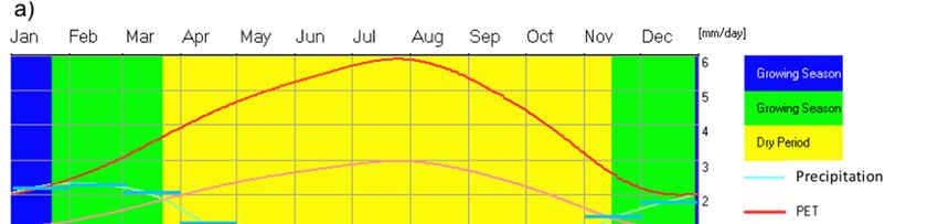
The band of warm ocean water that develops inter-annually in the central and east-central
    equatorial Pacific, El Niño Southern Oscillation (ENSO), is the major source of climate variability
    affecting different parts of the world [72,73]. However, the Pacific Decadal Oscillation (PDO), i.e., the
    variation of sea surface temperatures in the Pacific Ocean north of 20° N with a warm phase and a
    cool2019,
Climate  phase7, 6can modulate the interannual relationship between ENSO and the global climate [74]. The         9 of 17
    teleconnection of precipitation in California with climate phases such as the PDO and ENSO are
    reported in literature. A warm (positive) PDO is thought to have a similar spatial precipitation
      When examining
    signature    as a positivethe  projection
                                ENSO            of PDSI
                                       (wet in the        overSouthwest
                                                    American     four futureanddecades
                                                                                dry in the(2015–2054),   the ensemble
                                                                                            Pacific Northwest),  and
mean    value    (Figure   6, black  bold   curve)  is observed    to roughly   lie around   the
    a cool (negative) PDO has a similar signature as a negative ENSO [75]. ENSO has an important  “incipient  drought”
class,  approaching
    influence           “mild drought”
                on the rainfall  regime in around     2030,
                                             California andalthough
                                                             most of thesome
                                                                          U.S.members
                                                                               with mostpush    to “extreme
                                                                                           dramatic           drought”.
                                                                                                     impacts during
Around    2020 and
    the winter         2036,
                  season      PDSI
                          [76]. Theforecasts
                                    PDO is alsoapproach
                                                   relevant“near  normal”
                                                             because        with
                                                                      its cool    some
                                                                               phase     members
                                                                                     is linked      which
                                                                                               to dry      are inclined
                                                                                                       conditions in
up Southern     California
    to “incipient            and neighboring
                      wet spell”.               states
                                   After the year      [77].the
                                                     2040,   A plot
                                                                PDSIof resumes
                                                                       all available ENSO time
                                                                                 decreasing   andseries jointly
                                                                                                    remains     withthe
                                                                                                             below
    the PDOdrought”
“incipient     and PDSIfor time  series is shown in Figure 7.
                              years.

      Figure   6. Evolution
          Figure  6. Evolutionof of
                                 observed
                                    observedannual
                                             annualPDSI
                                                    PDSI(black
                                                         (blackcurve)
                                                                curve)with
                                                                        withits
                                                                              itssmoothed
                                                                                  smoothed 11-year    Gaussian filter
                                                                                             11-year Gaussian    filter in
      boldin blue
              boldcurve
                    blue (1942–2014),    and exponential
                           curve (1942–2014),            smoothing
                                                and exponential       forecastsforecasts
                                                                 smoothing       (2015–2054)    with plume
                                                                                         (2015–2054)     withprediction
                                                                                                               plume
      (light  gray) and
          prediction      thegray)
                      (light  ensemble    mean
                                    and the     valuemean
                                            ensemble (boldvalue
                                                           black(bold
                                                                  line).black
                                                                         PDSIline).
                                                                                classes
                                                                                    PDSIareclasses
                                                                                             also reported.
                                                                                                   are also reported.

3.4. Comparison with the Transfer Function Modelling Approach
     The band of warm ocean water that develops inter-annually in the central and east-central
equatorial Pacific, El Niño Southern Oscillation (ENSO), is the major source of climate variability
affecting different parts of the world [72,73]. However, the Pacific Decadal Oscillation (PDO), i.e.,
the variation of sea surface temperatures in the Pacific Ocean north of 20◦ N with a warm phase and
a cool phase can modulate the interannual relationship between ENSO and the global climate [74].
The teleconnection of precipitation in California with climate phases such as the PDO and ENSO
are reported in literature. A warm (positive) PDO is thought to have a similar spatial precipitation
signature as a positive ENSO (wet in the American Southwest and dry in the Pacific Northwest),
and a cool (negative) PDO has a similar signature as a negative ENSO [75]. ENSO has an important
influence on the rainfall regime in California and most of the U.S. with most dramatic impacts during
the winter season [76]. The PDO is also relevant because its cool phase is linked to dry conditions in
Southern California and neighboring states [77]. A plot of all available ENSO time series jointly with
the PDO and PDSI time series is shown in Figure 7.
     Sample cross-correlation functions (Figure 8) show that, among all ENSO indices, the ONI series
produced the highest cross-correlation with the PDSI series at a lag of −1 (=0.43), with the ONI series
leading by one time step (one year) the PDSI series. However, since this series is rather short (available
from 1950 onwards), we selected the next highly correlated series with PDSI, i.e., el Niño3.4 index
(=0.35 at lag −1), with the Niño3.4 series leading the PDSI series. Since the PDO time series is available
from year 1900, this was considered the initial year for the analysis. The model training period was the
interval 1900–1953 and the model validation period was the interval 1954–2014. The latter coincides
with the validation period used for the ES approach (Section 3.3). An ARIMA model was fitted to the
PDO series for the training period. An autoregressive model of order 1 (AR(1)) was adequate for the
series. Figure 9a2 presents the sample cross-correlation function (CCF) between the PDO series (X)
and the PDSI series (Y), and the sample CCF between the pre-whitened X series (residuals after fitting
an ARIMA model), with the filtered Y series (after applying the AR(1) filter) presented in Figure 9a1).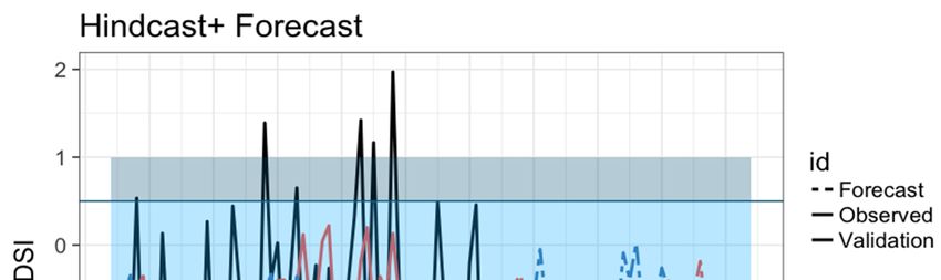
Climate 2019, 7, 6                                                                                                        10 of 17
      Climate 2018, 6, x FOR PEER REVIEW                                                                       10 of 18

      Figure    7. Time7. series Time
            Figure                   of PDO, series
                                                ENSO indicesof    (source:
                                                                     PDO, https://www.esrl.noaa.gov/psd/data/
                                                                                ENSO         indices       (source:
            https://www.esrl.noaa.gov/psd/data/climateindices/list)
      climateindices/list)    and PDSI. MEI-1871 and MEI-1950 are      andthe
                                                                            PDSI. MEI-1871 ENSO
                                                                              Multivariate  and MEI-1950    are the
                                                                                                    Index series  starting
            Multivariate
      in 1871   and 1950 ENSO    Index seriesindices
                           simultaneously;     startingNiño1+2,
                                                        in 1871 and  1950 Niño34
                                                                 Niño3,   simultaneously; indices
                                                                                  and Niño4    are Niño1+2,
                                                                                                   the meanNiño3,
                                                                                                             Sea Surface
            Niño34 and
      Temperature         Niño4 areinthe
                        anomalies        mean
                                       the    Sea Ocean
                                           Pacific Surfaceregions:
                                                            Temperature
                                                                    0–10anomalies  in the
                                                                          S, 90 W–80   W; Pacific
                                                                                          5 N–5Ocean
                                                                                                  S, 150regions:
                                                                                                         W–90 W; 0– 5 N–5
            10 S, 90 W–80 W; 5 N–5 S, 150 W–90 W; 5 N–5 S, 170–120 W; 5 N–5 S, 160 E–150 W, respectively; ONI
      S, 170–120 W; 5 N–5 S, 160 E–150 W, respectively; ONI is the Oceanic Niño Index; PDO is the Pacific
    Climate 2018,
            is the6,Oceanic
                     x FOR PEER
                             NiñoREVIEW
                                  Index; PDO is the Pacific Decadal Oscillation; SOI is the Southern Oscillation 11 of 18
      Decadal Oscillation; SOI is the Southern Oscillation Index.
            Index.

            Sample cross-correlation functions (Figure 8) show that, among all ENSO indices, the ONI series
      produced the highest cross-correlation with the PDSI series at a lag of −1 (=0.43), with the ONI series
      leading by one time step (one year) the PDSI series. However, since this series is rather short
      (available from 1950 onwards), we selected the next highly correlated series with PDSI, i.e., el Niño3.4
      index (=0.35 at lag −1), with the Niño3.4 series leading the PDSI series. Since the PDO time series is
      available from year 1900, this was considered the initial year for the analysis. The model training
      period was the interval 1900–1953 and the model validation period was the interval 1954–2014. The
      latter coincides with the validation period used for the ES approach (Section 3.3). An ARIMA model
      was fitted to the PDO series for the training period. An autoregressive model of order 1 (AR(1)) was
      adequate for the series. Figure 9a2 presents the sample cross-correlation function (CCF) between the
      PDO series (X) and the PDSI series (Y), and the sample CCF between the pre-whitened X series
      (residuals after fitting an ARIMA model), with the filtered Y series (after applying the AR(1) filter)
      presented in Figure 9a1).

      Figure 8. Sample
         Figure        cross-correlation
                8. Sample cross-correlationfunctions
                                             functions between  the PDSI
                                                       between the  PDSIseries
                                                                           seriesand
                                                                                  andallallENSO
                                                                                            ENSO  indices
                                                                                                indices   shown
                                                                                                        shown in in
      Figure 7. Numbers
         Figure 7. Numbersindicate
                            indicatethe
                                      theassociated
                                          associatedlag
                                                     lagat
                                                        at the
                                                           the peak value.
                                                               peak value.

      Similarly, an ARIMA model was fitted to the El Niño3.4 series for the training period.
An autoregressive model of order 2 (AR(2)) was adequate for the series. Figure 10b1 presents the
sample cross-correlation function (CCF) between El Niño 3.4 series (X) and the PDSI series (Y), and
the sample CCF between the pre-whitened X series (residuals after fitting an ARIMA model) and
the filtered Y series (after applying the AR(2) filter) in Figure 10b1 . Figure 9b1,b2 show a significant
spike at lag = −1 for the CCF between Niño3.4, and PDSI series and PDO and PDSI series. After
filtering the input and output time series to discard the autocorrelation effects, Figure 9a1,a2 show
the persistent significant leading impact of the Niño3.4 and the PDO series on the PDSI series one

          Figure 9. (a1) Sample cross-correlation function (CCF) between the pre-whitened Pacific Decadal
Climate 2019, 7, 6 11 of 17
year in advance (lag = −1). From the sample CCF functions and according to Box and Jenkins [42],
a transfer function model of order (r1 , s1 , d1 ) = (1, 1, 1) for input series X1 (t) = Niño3.4, and order
(r2 , s2 , d2 ) = (1, 0, 1) for input series X2 (t) = PDO, was proposed for this data set. In this case
α1 ( B) = (δ01 + δ11 B) B1 / 1 − ω11 B1 and α2 ( B) = (δ02 ) B1 / 1 − ω12 B1 .
The final model to be fitted is of the form:
Yt = α1 Yt−1 + α2 Yt−2 + α3 Nino3.4t−1 + α4 Nino3.4t−2 + α5 PDOt−1 + ηt (5)
Following Shumway and Stoffer [43], this model was initially fitted by least squares and the
ARIMA model associated to the estimated residuals η was identified. As a second step, the model
was refitted assuming autocorrelated errors following an ARIMA model with order identified in the
previous step.8. Figure
Figure Sample 10 shows the autocorrelation
cross-correlation and
functions between thepartial autocorrelation
PDSI series and all ENSOfunction of theinestimated
indices shown
residuals, suggesting a white noise structure with no additional
Figure 7. Numbers indicate the associated lag at the peak value. refitting required.
Climate 2018, 6, x FOR PEER REVIEW 12 of 18
Following Shumway and Stoffer [43], this model was initially fitted by least squares and the
ARIMA
Figure model (a1)associated to the estimated residuals between
was identified. As a second step, the model
Figure 9.9.(a1) Sample cross-correlation
Sample cross-correlation function
function(CCF)
(CCF) between thethe
pre-whitened
pre-whitened Pacific Decadal
Pacific Decadal
wasOscillation
refitted assuming
(PDO)seriesautocorrelated
series denoted
denoted as errors following an ARIMA model with order identified in the
Oscillation (PDO) as XXand
andthe
thefiltered
filteredPDSI
PDSI series denoted
series denotedas Y
asfor
Y the
for training period;
the training period;
previous
(a2)the step.
thesample Figure
sampleCCF 10
CCFbetween shows
between the the
the PDO autocorrelation and partial autocorrelation function of the
(a2) PDOseries
seriesand
andthethePDSI
PDSIseries; (b1)
series; CCF
(b1) pre-whitened
CCF pre-whitened Niño3.4 and and
Niño3.4
estimated residuals, suggesting a white noise structure with no additional
the filtered PDSI; (b2) the sample CCF between the Niño3.4 series and the PDSI series. refitting required.
the filtered PDSI; (b2) the sample CCF between the Niño3.4 series and the PDSI series.
Similarly, an ARIMA model was fitted to the El Niño3.4 series for the training period. An
autoregressive model of order 2 (AR(2)) was adequate for the series. Figure 10b1 presents the sample
cross-correlation function (CCF) between El Niño 3.4 series (X) and the PDSI series (Y), and the
sample CCF between the pre-whitened X series (residuals after fitting an ARIMA model) and the
filtered Y series (after applying the AR(2) filter) in Figure 10b1. Figure 9b1,b2 show a significant spike
at lag = −1 for the CCF between Niño3.4, and PDSI series and PDO and PDSI series. After filtering the
input and output time series to discard the autocorrelation effects, Figure 9a1,a2 show the persistent
significant leading impact of the Niño3.4 and the PDO series on the PDSI series one year in advance
(lag = −1). From the sample CCF functions and according to Box and Jenkins [42], a transfer function
model of order ( , , ) = (1,1,1) for input series ( ) = Niño3.4, and order ( , , ) =
(1,0,1) for input series () = , was proposed for this data set. In this case ( ) = ( +
) /(1 − ) and ( ) = ( ) /(1 − ).
The final model to be fitted is of the form:
= + + 3.4 + 3.4 + + (5)
Figure (a) Cross-correlation
10. 10.
Figure and (b)
(a) Cross-correlation andpartial autocorrelation
(b) partial functions
autocorrelation (ACF and
functions PACF,
(ACF andrespectively)
PACF,
of the estimatedofresiduals
respectively) (η̂t ) for
the estimated (^ )model.
the fitted
residuals for the fitted model.
Figure 1111
Figure compares
comparesthe theobserved
observedvalues
values (black line) with
(black line) withthe
thefitted
fittedvalues
valuesforfor
thethe training
training period
period
(blue line)
(blue and
line) thethe
and observed
observedvalues
valueswith
withthe
the fitted values for
fitted values forthe
thevalidation
validationperiod
period (red
(red line).
line). TheThe
95%95%
prediction intervals
prediction intervalsare also
are alsoshown
shownininthe
theanalysis.
analysis.Figure 10. (a) Cross-correlation and (b) partial autocorrelation functions (ACF and PACF,
respectively) of the estimated residuals (^ ) for the fitted model.
Figure 11 compares the observed values (black line) with the fitted values for the training period
(blue line) and the observed values with the fitted values for the validation period (red line). The 95%
Climate 2019, 7, 6 12 of 17
prediction intervals are also shown in the analysis.
Figure Observed
11.11.
Figure ObservedPDSI
PDSItime
timeseries
series(black
(black line)
line) with the training
with the trainingdataset
datasettotobuild
buildthethe model
model (blue
(blue
line) for the period 1900–1953, including the filtered observed values (navy blue). Also
line) for the period 1900–1953, including the filtered observed values (navy blue). Also comparison comparison
between
between thethe
observed
observedvalues
values(black
(blackline)
line) and
and predicted valueswith
predicted values withthe
theTF
TFmodel
model forfor
thethe validation
validation
period (1954–2014)
period (red
(1954–2014) line),
(red line),including
includingthe
thecorresponding 95% confidence
corresponding 95% confidenceintervals
intervals(red
(red dash).
dash).
RMSERMSE = 1.0
= 1.0 and
andMASE
MASE==0.950.95during
during the
the validation periodindicate
validation period indicatethat
that the
the TFM
TFM provided
provided an an
improvement
improvement over the
over naive
the naiveforecast.
forecast.Considering that in
Considering that in this
thiscase
casethe
thetraining
training period
period (1900–1953)
(1900–1953) is is
much
much shorter
shorter in in comparisonwith
comparison withthe
thetraining
training period
period used
used forforthe
theESESmethod
method(1800–1953),
(1800–1953), thethe
TMS TMS
Climate 2018, 6, x FOR PEER REVIEW 13 of 18
provides
provides a competitive
a competitive approachasasa aforecasting
approach forecastingmethod
methodfor forthe
the PDSI
PDSI series. The
The histogram
histogramand andQ- Q-Q
Q plots
plots of the ofresiduals
the residuals between
between the the predicted
predicted and and observed
observed values
values forfor
the the PDSItime
PDSI timeseries
seriesduring
duringthe
the validation period shows a satisfactory performance with an approximate normal distribution of
validation period(Figure
the residuals shows 12).
a satisfactory performance with an approximate normal distribution of the
residuals (Figure 12).
Figure 12. Residual histogram and normal Q-Q plot between the PDSI predicted values and observed
PDSIFigure 12. Residual
time series for the histogram
validationand normal
period Q-Q plot between the PDSI predicted values and observed
(1954–2014).
PDSI time series for the validation period (1954–2014).
3.5. Ensemble Forecast with the Transfer Function Model
3.5. Ensemble Forecast with the Transfer Function Model
Once the adequacy of the model was assessed, the model was trained over the period 1900–2014
to produce Once the adequacy
a simulation of the
plume of model
annualwas assessed,
PDSI values the
for model was trained
the period over El
2015–2054. theNiño3.4
period 1900–2014
series and
the PDO series were jointly simulated first, by using a multivariate ARIMA [78] model thatseries
to produce a simulation plume of annual PDSI values for the period 2015–2054. El Niño3.4 and
considers
the PDO series were jointly simulated first, by using a multivariate ARIMA [78] model that considers
dependence between the two series. The simulated values were included as external covariates for the
dependence between the two series. The simulated values were included as external covariates for
PDSI model trained over the period 1900–2014. Simulations are presented in Figure 13 from a model
the PDSI model trained over the period 1900–2014. Simulations are presented in Figure 13 from a
of the form:
model of the form:
Yt = α1=
Yt−1 + α2+Yt−2 + α+ t −1 + +
3 Nino3.43.4 α4 Nino3.4 t−2 ++α5 PDOt−1 +
3.4 + ηt (6)(6)the PDO series were jointly simulated first, by using a multivariate ARIMA [78] model that considers
dependence between the two series. The simulated values were included as external covariates for
the PDSI model trained over the period 1900–2014. Simulations are presented in Figure 13 from a
model of the form:
Climate 2019, 7, 6 = + + 3.4 + 3.4 + + 13 of 17
(6)
Figure
Figure13.13.Observed PDSI time
Observed PDSI timeseries
series (black
(black line)
line) withwith the simulation
the simulation plume plume (grey
(grey lines) forlines) for the
the period
period 2015–2054,
2015–2054, including
including the filtered
the filtered observed
observed series (navy-blue
series (navy-blue line), theline), the of
median median of the simulated
the simulated values
values (thick
(thick greygrey
line)line)
andand
the the
2.5%2.5% (bottom
(bottom dashed
dashed line)line)
andand 97.5%
97.5% quantile
quantile (top(top dashed
dashed line)
line) of the
of the
simulated
simulated values.
values.
TheThe
inter-decadal
inter-decadal cycles observed
cycles observed inin
thetheensemble
ensembleforecast
forecastfrom
fromthe
theES
ESapproach
approach(Figure
(Figure5)5)are
arenot
present
not in this
present case
in since
this a
case seasonal
since
Climate 2018, 6, x FOR PEER REVIEW a component
seasonal was
component not considered
was not in the
considered model.
in the Figure
model. 14 compares
Figure
14 of 14
18
thecompares
two approaches
the two (ES ad TFM)(ES
approaches in the
ad validation
TFM) in theand forecastand
validation periods. With
forecast ES, theWith
periods. projections
ES, the of
projections
with
PDSI over fouroffuture
episodes PDSI overdrought”,
of “mild four(2015–2054)
decades future decades
while the (2015–2054)
lie projections
around liethe
the of around the “incipient
TFMdrought”
“incipient remain class,drought”
around class, of
the “incipient
with episodes
drought”
“mild drought”,region.
while the projections of the TFM remain around the “incipient drought” region.
Figure Comparison
14.14.
Figure Comparisonbetween
between estimates
estimates from the exponential
from the exponentialsmoothing
smoothingmodel
model (ESM)
(ESM) and
and thethe
Transfer Function
Transfer model
Function model(TFM)
(TFM)for
forboth
both the
the validation period(1954–2014)
validation period (1954–2014)and
and the
the forecast
forecast period
period
(2015–2054).
(2015–2054).
3.6. Limitations and Perspectives
3.6. Limitations and Perspectives
Droughts
Droughts occur
occurover
overlong-time
long-timespans,
spans, and
and their timingisisdifficult
their timing difficulttotoidentify
identify and
and predict.
predict. This
This
paper takes the challenge to examine a strategy for structuring knowledge about
paper takes the challenge to examine a strategy for structuring knowledge about drought dynamics, drought dynamics,
forfor
useuse
in in
annual
annualPDSI
PDSIextrapolation
extrapolationforforthe
the coming decades.Extrapolation
coming decades. Extrapolationsufferssuffers when
when a time
a time series
series
is subject
is subjectto to
shocks
shocksorordiscontinuities.
discontinuities. Few
Few extrapolation methodsaccount
extrapolation methods account forfor discontinuities
discontinuities [79].[79].
Instead, when
Instead, whendiscontinuities
discontinuities occur, extrapolation
occur, extrapolation may lead
may to large
lead forecast
to large errors.
forecast For For
errors. example, ENSO
example,
andENSO
PDO canand lead
PDOtocan
strong
leadupward or downward
to strong upward or trends
downwardof drought
trendsindex values index
of drought and frequencies
values and[80].
frequencies
According with[80]. According
Sheffield with Sheffield
and Wood [81], it isand Wood that
plausible [81],thermal
it is plausible
impacts that
onthermal
droughtimpacts on in
frequency
thedrought
long term frequency in to
are likely thedominate
long termprecipitation
are likely to changes.
dominate We precipitation
could thus changes.
expect We could thusand
a monotonic
expecttemperature
positive a monotonic change
and positive temperaturedrought
with increasing change with increasing
frequency acrossdrought
a range frequency
of droughtacross a
metrics
range of drought metrics by the late 21st century. However, the future direction of PDSI series
remains uncertain, because uncertain is the direction of its causal forces (temperature and
precipitation). This is a challenge in PDSI future extrapolation. Forecasts from Esfahani and Friedel
[82] suggested the likelihood for the current moderate drought in California to shift to a mid-range
condition in 2020 and a constant level of PDSI towards 2060. These authors advocate that CaliforniaYou can also read