Decision Analysis of Disturbance Management in the Process of Medical Supplies Transportation after Natural Disasters - MDPI
←
→
Page content transcription
If your browser does not render page correctly, please read the page content below
International Journal of
           Environmental Research
           and Public Health

Article
Decision Analysis of Disturbance Management in the
Process of Medical Supplies Transportation after
Natural Disasters
Yuhe Shi and Zhenggang He *              ID

 School of Transportation and Logistics, Southwest Jiaotong University, Chengdu 610031, China;
 SHI681242@163.com
 * Correspondence: hezhenggang@swjtu.edu.cn; Tel.: +86-028-8763-4338

 Received: 19 June 2018; Accepted: 31 July 2018; Published: 3 August 2018

 Abstract: Public health emergencies, such as casualties and epidemic spread caused by natural
 disasters, have become important factors that seriously affect social development. Special medical
 supplies, such as blood and vaccines, are important public health medical resources, and the
 cold-chain distribution of medical supplies is in a highly unstable environment after a natural
 disaster that is easily affected by disturbance events. This paper innovatively studies the distribution
 optimization of medical supplies after natural disasters from the perspective of disturbance
 management. A disturbance management model for medical supplies distribution is established
 from two dimensions: time and cost. In addition, a hybrid genetic algorithm is introduced to solve
 the model. Disturbance recovery schemes with different weight coefficients are obtained through
 the actual numerical experiments, and experimental results show the effectiveness of the proposed
 model and algorithm. Finally, we discuss the formulation of weight coefficients in the case of
 emergency distribution and general distribution, which provide a reference for emergency decisions
 in disturbance events.

 Keywords: natural disasters; medical supplies transportation; cold-chain distribution; disturbance
 management; hybrid genetic algorithm

1. Introduction
     In recent years, various natural disasters have occurred frequently, such as Hurricane Katrina in
2005, the Wenchuan Earthquake in 2008, and the Typhoon in the Philippines in 2013 [1–4]. After natural
disasters, special medical supplies such as blood and vaccines are the key to reducing casualties
and fighting infectious diseases. The efficient distribution of these special medical supplies is of
great importance to public health and individual health. In general, special medical supplies, such
as blood and vaccines, are extremely sensitive to temperature, and the quality of their cold-chain
distribution is positively correlated with medical efficacy [5]. Only under specific temperatures or
external environment conditions can it be ensured that medical supplies will not lose efficacy or
deteriorate. In the circulation process of medical supplies, the cold-chain logistics are clearly important
for ensuring the immune efficacy and safety of medical supplies [6]. However, the process of cold-chain
distribution, which has the characteristics of high uncertainty, dynamics, and interactions, is easily
affected by a multitude of disturbance events, including demand changes, road interruptions caused
by natural disaster, vehicle refrigeration equipment failure, and so on, thus leading to the original
distribution plan being affected, and even interruptions to the cold-chain.
     Therefore, it is important to address disturbance events scientifically after the occurrence of
natural disasters. After a disturbance event occurs, the distribution order of the remaining service

Int. J. Environ. Res. Public Health 2018, 15, 1651; doi:10.3390/ijerph15081651   www.mdpi.com/journal/ijerph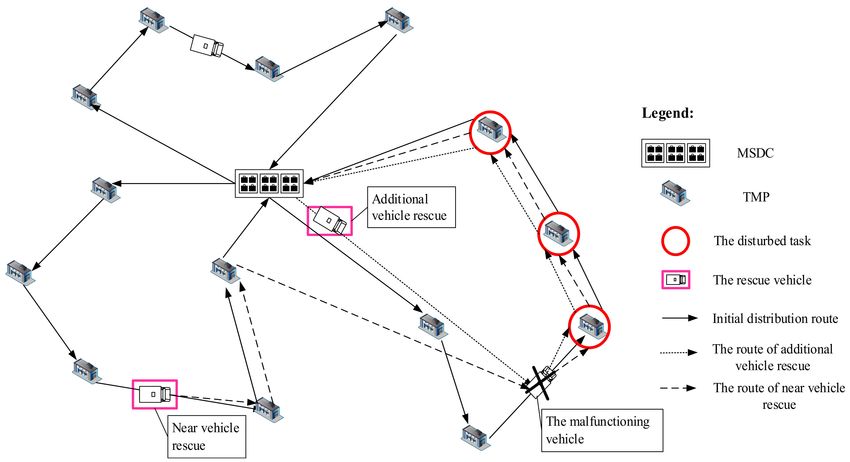
Int. J. Environ. Res. Public Health 2018, 15, 1651                                                 2 of 18

objects should be adjusted, which is bound to result in a chain reaction and cause system confusion.
At this point, we need to consider the impact of the disturbance on the entire cold-chain logistics
and distribution system to generate an adjustment program that minimizes the system disturbance.
Based on this, if the distribution quality and efficiency of medical supplies need to be ensured
simultaneously, the medical supplies’ cold-chain distribution problem will become more complicated.
How to effectively address disturbance events that lead to the interruption of the cold-chain and
maintain the safety and efficiency of medical supplies are urgent problems that need to be solved in
medical supply cold-chain distribution after natural disasters.
     The remaining parts of this paper are organized as follows. In the next section, a literature review
on the disturbance management problem as well as the logistics and distribution of medical supplies
is presented. Section 3 discusses the construction of the disturbance management model for medical
supplies distribution (DMMSD). The hybrid genetic algorithm is introduced to solve the model in
Section 4. Section 5 gives a numerical experiment and results analysis. Finally, Section 6 concludes this
paper and presents expectations for future work.

2. Literature Review
    Since the main idea of the current research is to study the distribution optimization of medical
supplies after natural disasters from the perspective of disturbance management, we review the
studies in two fields: disturbance management in transportation and distribution optimization of
medical supplies.

2.1. Disturbance Management in Transportation
     There have been a large number of disturbance events across all walks of life. At present,
disturbance management has become a hot issue for scholars to study, including aspects such
as aviation disturbance management [7,8], supply chain disturbance management [9,10], machine
scheduling disturbance management [11,12], railway scheduling disturbance management [13], and so
on. As early as the 1970s and 1980s, research on disturbance had begun. The disturbance management
was first applied in the aviation field by Yu [14], and since then, many research results have been
produced on this classical optimization problem. There have also been many achievements in research
on the disturbance management of logistics distribution. Zeimpekis et al. [15] classified the disturbance
problem in logistics distribution and set up a mathematical model with the objectives of minimizing
the delay cost and serving the largest number of customers. A disturbance recovery model of logistics
distribution was established by Potvin et al. [16] to solve the problems of new customer demand and
travel time disturbance, and they introduced an insertion algorithm for this model. Tiguiguchi and
Shimamoto [17] studied the influence of uncertain vehicle traveling time on formulating a distribution
plan and conducted an experiment that introduced changeable traveling time as the disturbance
variable. Ruan and Wang [18] constructed a disturbance recovery model for the joint delivery of
emergency medical supplies to analyze the disturbance of an emergency logistics system due to
transfer point changes, and they designed a genetic algorithm to solve the model. Ding et al. [19]
measured disturbance based on the prospect theory, and a multi-objective disturbance management
model was proposed. Combined with related theories in behavioral science, Liu et al. [20] discussed
the influence of disturbance events on an emergency logistics system from three aspects: demand
point, decision maker, and logistics worker. In conclusion, many scholars have studied disturbance
management in different transportation environments, but there is no literature related to disturbance
events in the transportation of medical supplies.

2.2. Distribution Optimization of Medical Supplies
     Another study related to this article is the logistics and distribution of medical supplies which
requires high safety and punctuality. Based on the needs of theoretical research and practical
application, scholars have conducted a great deal of research on this pertinent problem. According to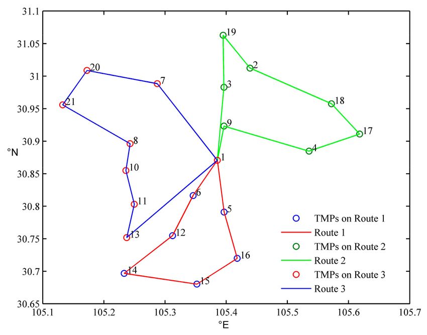
Int. J. Environ. Res. Public Health 2018, 15, 1651                                                   3 of 18

the characteristics of emergency medical blood, Ramezanian et al. [21] proposed an optimization model
for blood supply chain design in both deterministic and robust environments, and the application of
the proposed model was evaluated by a case study in Tehran. The target functions in the integrated
optimization model for the selection of emergency blood transfer points and transport routes proposed
by Wang et al. [22] included having a minimum arrival time for emergency blood, maximum freshness
at the time of reception, and minimization of the total transportation cost. A genetic algorithm
for local neighborhood optimization was designed in their study. Chen et al. [23] considered the
time constraints from the perspective of joint distribution and established an optimization model
for multi-species cold-chain vaccine distribution. To minimize the maximum arrival time and the
average arrival time, Campbell et al. [24] set up a path optimization model for vehicles with emergency
supplies and used a local search algorithm to solve the model. Taking the Haiti earthquake in 2010 as
an example, Battini et al. [25] developed a last mile distribution optimization model for emergency
supplies and analyzed the optimization results under different scenarios. Ruan et al. [26] presented a
two-stage approach for the intermodal transportation of medical supplies by “helicopters and vehicles”
in large-scale disaster responses. Although there has been a large number of studies on the distribution
optimization of medical supplies, few scholars have studied the distribution optimization of special
medical supplies after natural disasters based on the perspective of disturbance management.
      In short, as important medical supplies that are relevant to public health, the cold-chain
distribution environments of blood and vaccine are highly unstable and vulnerable to disturbance.
However, there have been few studies on the disturbance management of medical supply distribution.
Taking vehicle breakdown (failure of refrigerating equipment) in the distribution process as an
example, the idea of disturbance management is used to study the disturbance events in the cold-chain
distribution of medical supplies in this paper. In contrast to the single-objective optimization model,
we measure the disturbance from two dimensions, time and cost, and establish a disturbance
management model for medical supply distribution (DMMSD) with minimum cost and time
disturbance as the objective functions, and we design a hybrid genetic algorithm to solve this problem.
Then, based on an actual case, the distribution schemes of disturbance recovery under different weights
are obtained by our model and algorithm, thus providing a reference for the decision-making process
of medical supply cold-chain distribution disturbance management.

3. Model Formulation

3.1. Problem Description
      After a disaster, the rescue work in the first phase mainly involves the repair of basic facilities,
such as road traffic and communication, as well as the simultaneous rescue of survivors. Then, on the
basis of unimpeded communication and roads, a large number of medical materials are transported
into the disaster area to reduce casualties and reduce the risk of secondary disasters caused by the
outbreak of an epidemic situation [27,28]. This is called the second phase of post-disaster rescue [26,29],
which is the background of this paper and the application environment for the DMMSD.
      The problem studied in this paper can be described as follows. In the second phase of rescue
after a natural disaster, the Medical Supplies Distribution Center (MSDC) distributes medical supplies
to a number of temporary medical points (TMPs) through refrigerated trucks, and the locations of
TMPs are known. There are same types of refrigerated vehicles, and medical supplies that require the
same distribution temperature are transported by the same vehicle. Each refrigerated vehicle starts
from the MSDC and will return to the MSDC after delivering the medical supplies to the designated
TMPs along a known distribution route. The TMPs have time windows in which they receive services,
which means the medical supplies are required to reach the TMP within a certain time interval. In the
absence of any disturbances, the initial known delivery schemes can meet the requirements of the
TMPs and the load limits of the vehicles. When a disturbance event occurs (taking vehicle breakdown
and refrigeration equipment failure during the delivery process as an example), the problems that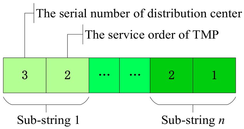
Int. J. Environ. Res. Public Health 2018, 15, 1651                                                  4 of 18

need to be resolved are as follows: the recovery of normal operation of the system as soon as possible,
the completion of the distribution tasks with consideration of the interests of multiple stakeholders,
and the minimization of the time disturbance and cost at the same time.
      After a natural disaster, during the process of cold-chain distribution, any one of many factors,
such as vehicles, cargoes, paths, demands and others, may be disturbed, which will influence the
distribution task. Disturbance events can interrupt the cold-chain. If we continue to deliver medical
supplies according to the initial schemes formulated before the occurrence of the disturbance event,
inevitably some of the demand points will not receive the expected service, and the immune efficacy of
the medical supplies will be affected. Therefore, it is necessary to construct a disturbance management
model and to adjust the distribution schemes according to the disturbance event to utilize adjustment
schemes that minimize the disturbance of the system. In this paper, disturbance management in the
cold-chain logistics distribution of medical supplies is studied with the example of vehicle breakdown
in the distribution process.
      In short, the real environment after natural disasters is more complicated. In order to model the
situation after a natural disaster and make scientific quantitative decision analysis, we refer to the
literature [30–42], and make the following assumptions:

•     As mentioned above, after a natural disaster, any one of a number of factors, such as vehicles,
      cargoes, paths, demands, and others, may be disturbed in the process of cold-chain distribution,
      which will influence the distribution task. In this paper, we assume that the transport capacity
      is disturbed (vehicle breakdown) to study the distribution optimization after a single type of
      disturbance event occurs.
•     After a natural disaster, the rescuers dispatched by the government restore basic communication
      and traffic as soon as possible and rescue the survivors simultaneously. On the basis of unimpeded
      communication and roads, medical supply distribution can be carried out to ensure timely medical
      assistance to the injured and to reduce the risk of secondary disasters caused by the outbreak of
      epidemic situation. So, in this paper, we assume that the communication and roads are basically
      unimpeded during the distribution process of medical supplies.
•     The location and service time windows of TMPs are known.
•     The initial distribution scheme is known, and the same type of refrigerated vehicle is used.
•     In a distribution task, each TMP is only served once.

3.2. Disturbance Processing Strategy
      In the distribution process of medical supplies, a vehicle is not able to continue driving and
the refrigerator cannot continue to work normally—the vehicle breaks down and the issue cannot
be resolved in a short period of time. After the vehicle fails, the pending delivery cargoes and
unfinished delivery tasks will be affected. The subsequent rescue mission includes picking up the
cargoes and completing the unfinished delivery tasks of the disturbed vehicle. If a disturbance occurs
to a distribution vehicle while the vehicle is on its way to the next TMP or the vehicle is servicing
a TMP, it is assumed that the location of the disturbed vehicle is the pseudo demand point and the
rescue vehicle needs to reach this location for rescue. If the vehicle fails when it is still at the MSDC,
only new vehicles can be dispatched to service the affected demand points.
      The problem studied in this paper involves the disturbance management of the vehicle routing
problem with time window (VRPTW); the cargoes need to be delivered in the time window required
by TMPs. Furthermore, because of the characteristics of the medical supplies, it is necessary to store
and transport them under certain temperature conditions. Thus, there are two kinds of rescue strategy:
(1) the additional vehicle rescue strategy, which means new vehicles in the MSDC are dispatched for
rescue in accordance with the original path, and (2) the near vehicle rescue strategy, which assumes
that the locations of the vehicles on the way to deliver cargoes are pseudo distribution centers when the
disturbance event occurs, and that the vehicles in the pseudo distribution centers are deployed to assist
Int. J. Environ. Res. Public Health 2018, 15, 1651 5 of 18
the disturbed vehicle to complete the remaining tasks. A schematic diagram of vehicle breakdown
rescue is shown in Figure 1.
Figure 1. A schematic diagram of vehicle breakdown rescue.
3.3. Parameters and Variables
According to the needs for building the model, this paper uses the following parameters and
variables, as shown in Table 1.
Table 1. The meanings of parameters and variables.
Parameters and Variables Meaning
E Collection of temporary medical points (TMPs)
CE Collection of TMPs that have been served when a disturbance event occurs
Collection of TMPs that have not been served when a disturbance
UE
event occurs
VE Collection of pseudo demand points
V Collection of distribution vehicles
R Collection of vehicles on their way to deliver cargoes
D Collection of vehicles at the Medical Supplies Distribution Center (MSDC)
0 Starting point of the vehicle
F End point of the vehicle after the delivery service is completed
V = R∪D Collection of all available vehicles
RF = UE ∪ VE Collection of task points after the disturbance event occurs
i, j ∈ E ∪ 0 ∪ F,
OP = (i, j, k) Original distribution scheme
k∈V
New distribution scheme, the collection of network nodes changes as
EP
E0 = RF ∪ {0, F }
a Total number of TMPs that have not been served
Total number of the vehicles on the way to deliver cargoes in the original
b
distribution schemeInt. J. Environ. Res. Public Health 2018, 15, 1651 6 of 18
Table 1. Cont.
Parameters and Variables Meaning
Collection of points, P = { p1 , p2 , . . . , p a+b+1 }, where { p1 , p2 , . . . , p a }
represents the TMPs that have not been served; p a+1 is the location of the
disturbed vehicle; { p a+2 , . . . , p a+b } represents the location of the vehicles on
P
the way to deliver cargoes when a disturbance event occurs, that is, the
pseudo distribution centers; p0 is the location of the MSDC, which is the
initial distribution center
dij Distance between pi and p j
s Speed of the refrigerated vehicles
Time that the temperature inside the refrigerated box goes up by 1 ◦ C when
t0
the refrigeration equipment fails to work
T0 Critical temperature at which the medical supplies approach deterioration
Temperature inside the refrigerated box when the refrigerated vehicle is
Tn
normal working
wi Service time of the vehicle for pi
ts Moment of the disturbance event occurs
DTki Time for vehicle k to reach TMP i in the original plan
DTki 0 Time for vehicle k to reach TMP i after adjusting the distribution scheme
Time window of TMP i, including the beginning and end point of the arrival
[ ETi , LTi ]
time required by the TMP
gi Medical supply demands of TMP i in the original distribution scheme
giEP Medical supply demands of TMP i after the disturbance event occurs
Qk Maximum load allowed for refrigerated vehicle k
QkEP Available load of vehicle k that is on its way to deliver cargo
Transportation cost for a unit of distance for a refrigerated vehicle from TMP i
Cij
to TMP j
L( EP) Collection of distribution path edge in the new scheme
L(OP) Collection of distribution path edge in the original scheme
The deviation parameter of the path, when (i, j, k) ∈ L(OP)/L( EP),
Lijk = −1 indicates the path edge between TMP i and TMP j is shown in the
original scheme but not in the new scheme; when
Lijk (i, j, k) ∈ L( EP)/L(OP),Lijk = 1 indicates the path edge between TMP i and
TMP j is shown in the new scheme but not in the original scheme; when
(i, j, k) ∈ L( EP) ∩ L(OP), Lijk = 0 indicates the path edge between TMP i and
TMP j is shown in both the original and new schemes
A 0–1 variable, xijk = 1 represents that vehicle k is driven from TMP i to TMP
xijk
j, otherwise xijk = 0
A 0–1 variable, zijk = 1 represents that vehicle k is driven from the pseudo
zijk
distribution center pi to demand point p j , otherwise zijk = 0
A 0–1 variable, z0jk = 1 represents that vehicle k is driven from the MSDC p0
z0jk
to demand point p j , otherwise z0jk = 0
3.4. Measurement of Disturbance
In this paper, the disturbance of vehicle breakdown is measured from two aspects: the arrival time
disturbance of the medical supplies and the cost disturbance of the distribution. Then, a multi-objective
function model with minimum cost and time disturbances is established.
3.4.1. The Cost Disturbance
After a disturbance event occurs, the original distribution plan is terminated, and a new
distribution plan is started. The cost disturbance is composed of the cost of the path change, the cost
of the additional new vehicle rescue, and the penalty cost that includes the penalty cost of failing toInt. J. Environ. Res. Public Health 2018, 15, 1651 7 of 18
serve the TMPs and the cost of breaking the required time window. We set C1 as the unit cost for a
new vehicle; C2 as the unit penalty cost for distribution failure; µ1 as the waiting cost per unit of time
when the vehicle arrives at the TMP in advance; and µ2 as the penalty cost per unit of time when the
vehicle is late to the TMP. The expression for cost disturbance is
minC = ∑ ∑ ∑ zijk Cij dij Lijk + ∑ ∑ z0jk C1 L0jk + ∑ ∑ ∑ C2 1 − xijk
k ∈ R i ∈ RF j∈ E0 k ∈ D j∈ RF k ∈V i ∈ RF j∈ E0
(1)
+∑ 0 , 0} + µ 0
∑ (µ1 max{ ETi − DTki 2 max{ DTki − LTi , 0})
k ∈V i ∈ RF
In Formula (1), max{ ETi − DTki 0 , 0} indicates the advanced arrival time for vehicle k with service
TMP i, and max{ DTki 0 − LTi , 0} indicates the amount of time by which vehicle k is late to service
TMP i.
3.4.2. The Time Disturbance
After a natural disaster, there are three situations for the time disturbance of medical supplies
arriving at the TMP: (1) the arrival time after adjusting the distribution scheme (DTki 0 ) is exactly the
same as the original planned arrival time (DTki ); (2) the arrival time after adjusting the distribution
scheme (DTki 0 ) is later than the original planned arrival time (DTki ); or (3) the arrival time after
adjusting the distribution scheme (DTki 0 ) is earlier than the original planned arrival time (DTki ).
The third situation has a positive impact on the TMP, but it is likely generated by delaying the delivery
time of other TMPs or increasing delivery vehicles, so we also regard it as a disturbance.
According to the analysis presented above, the disturbance of the medical supplies’ arrival time
for TMP i can be expressed as
λ( DTki − DTki 0 ), λ ∈ {−1, 0, 1} (2)
where λ is a symbolic variable. When DTki 0 = DTki , there is no arrival time disturbance in TMP i
(λ = 0); when DTki 0 > DTki , that is, the arrival time after adjusting the distribution scheme is later
than the originally planned arrival time (λ = 1); when DTki 0 < DTki , that is, the arrival time after
adjusting the distribution scheme is earlier than the originally planned arrival time (λ = −1). Then,
the arrival time disturbance of all of the TMPs can be obtained.
minT = ∑ ∑ λ( DTki − DTki 0 ), λ ∈ {−1, 0, 1} (3)
k ∈ RF i = Eki
where Eki is a collection of TMPs serviced by vehicle k in the original scheme.
3.5. The DMMSD Model Setting
In the second phase of post-disaster rescue, time and cost are the main targets followed by the
three subjects of medical supplies distribution (MSDC, TMP, and distribution operator) in the face of a
disturbance. Based on the analysis of disturbance in Section 3.4, the DMMSD model was constructed
as follows:
minC = ∑ ∑ ∑ zijk Cij dij Lijk + ∑ ∑ z0jk C1 L0jk + ∑ ∑ ∑ C2 1 − xijk
k ∈ R i ∈ RF j∈ E0 k ∈ D j∈ RF k ∈V i ∈ RF j∈ E0
(4)
+∑ ∑ (µ1 max{ ETi − DTki 0 , 0} + µ2 max{ DTki 0 − LTi , 0})
k ∈V i ∈ RF
minT = ∑ ∑ λ( DTki − DTki 0 ), λ ∈ {−1, 0, 1} (5)
k ∈ RF i = Eki
subject to
∑ ∑ xijk ∗ giEP ≤ QkEP ∀k ∈ V (6)
i ∈ RF j∈ E0
∑ ∑ xijk ≤ 1∀i ∈ RF (7)
j∈ E0 k ∈VInt. J. Environ. Res. Public Health 2018, 15, 1651 8 of 18
∑ ∑ z0jk ≤ | D | (8)
k ∈V j∈ RF
1(i, j, k) ∈ L( EP)/L(OP)
Lijk = 0 (i, j, k) ∈ L( EP) ∩ L(OP) (9)
−1(i, j, k) ∈ L(OP)/L( EP)
a + b +1
∑ xi(a+b+1)k = 1k = 1, 2, . . . , b (10)
i =1
( T0 − Tn )/t0 ≥ DTki 0 − ts , Tn ≤ T0 (11)
a + b +1 b
∑ ∑ xijk ti + wi + dij /s = t j j = 1, 2, . . . , a + 1
(12)
i =1 k =1
ETi ≤ ti + wi ≤ LTi i = 1, 2, . . . , n (13)
The model indicates that the objective of our problem is to minimize the deviation between the
adjusted and initial schemes, which means that the degree of disturbance to the system is minimal,
as shown in Expressions (4) and (5). Constraint (6) represents that the demands of TMPs cannot exceed
the current load capacity of the rescue vehicle after the disturbance event occurs. Each task point can
only be served once, and its operation is shown in constraint (7). The maximum number of available
vehicles for rescue is emphasized in constraint (8). Constraint (9) imposes the notion of the definition
of a path deviation parameter in the original and new schemes, including the path added in the new
scheme, the path deleted in the original solution, and the changeless path. Constraint (10) shows the
vehicle returning to the initial distribution center after finishing its service to the TMPs. Constraint (11)
ensures that the disturbed vehicle is rescued before the medical supplies lose efficacy or deteriorate.
The time window set for the TMPs must be met, which is imposed by constraints (12) and (13).
4. Algorithm Design
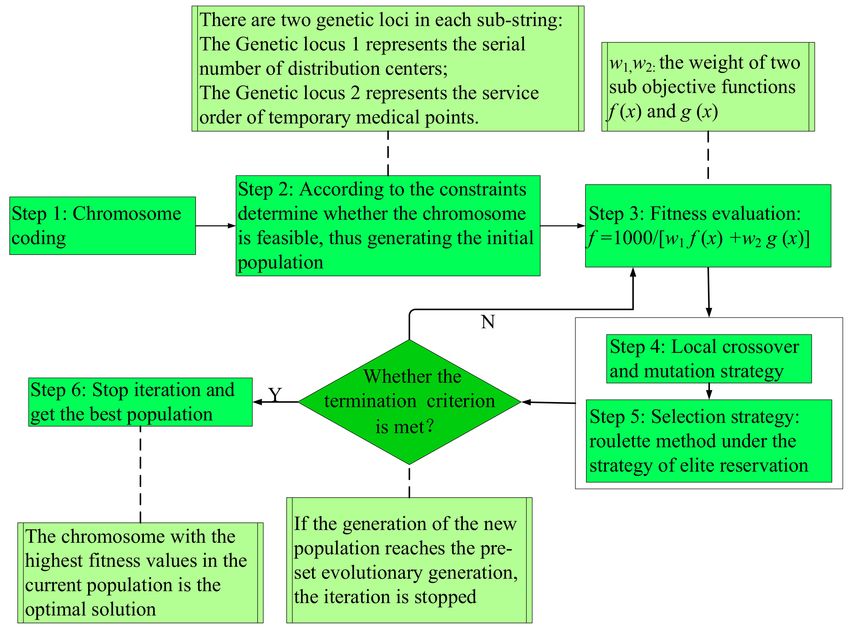
Based on the idea of the genetic algorithm [43–48], a hybrid genetic algorithm (HGA) for solving
the DMMSD model is designed in this section. The specific process is shown in Figure 2.
Figure 2. The specific process of the hybrid genetic algorithm.Int. J. Environ. Res. Public Health 2018, 15, 1651 9 of 18
Step 1: Chromosome coding. One chromosome represents a solution to the problem;
each chromosome consists of n gene strings, and each gene string represents the service status of a
TMP. There are two genetic loci in each substring: genetic locus 1 represents the serial number of the
distribution center and genetic locus 2 represents the service order of TMP. Taking the chromosome in
Figure 3 as an example, substring 1 indicates that TMP 1 is served by pseudo distribution center 3 in
the second order, and substring n indicates that TMP n is served by pseudo distribution center 2 in the
first order.
Figure 3. Example of chromosome coding.
Step 2: Initializing the population. To ensure that the algorithm performs the optimization in a
feasible solution space, each chromosome is decoded after it is generated in the process of population
initialization. The chromosome is judged by constraints (6)–(13). If all of the constraints are satisfied,
the chromosome is viable. Otherwise, new chromosomes will be regenerated through population
initialization or genetic evolution until M chromosomes are obtained.
Step 3: Evaluation of population fitness. In order to intuitively see the subtle changes in the fitness
value in the algorithm convergence graphs, we set the numeric value of the numerator to 1000. The
fitness function set in the HGA is as follows:
1000
f = (14)
w1 f ( x ) + w2 g ( x )
where w1 and w2 represents the weights of two sub-objectives, respectively.
Step 4: Crossover and mutation operation. According to the characteristics of the DMMSD model,
we designed a local crossover and mutation method to improve the evolutionary efficiency of the
algorithm. First, gene strings affected by disturbance are identified in two parent chromosomes.
Then, the identified gene strings and unidentified gene strings are implemented in the local crossover
(cross-probability, PC) and mutation operations (mutation probability, PM) separately to form progeny
chromosomes. Finally, it is determined whether the newly generated progeny chromosomes meet the
constraints until sufficient progeny chromosomes are constructed.
Step 5: Selection strategy. The roulette method under the strategy of elite reservation was chosen
as the selection strategy in this paper. When generating the next-generation population, the parental
population and the best individuals in the temporary population generated by crossover and mutation
operations are directly reserved to the offspring. The other individuals in the new population are
chosen from the parental and temporary populations by the roulette method.
Step 6: Termination conditions of the algorithm. The maximum iteration number of the genetic
algorithm LS is set. The algorithm stops iterating when gen > LS, where gen is the algorithm iteration.
5. Numerical Experimental Design
The numerical experiments include the following three parts: First, the example data from the
medical supplies distribution are used to verify the effectiveness of the DMMSD model in Section 5.1.
Second, we obtain the experimental results and import them into the actual map to analyze the results
in Section 5.2. Finally, the experimental results are discussed in Section 5.3.Int. J. Environ. Res. Public Health 2018, 15, 1651 10 of 18
This paper used MATLAB R2014a to implement the HGA, and all experiments in this paper
were evaluated on PCs with Intel® Core™ (Santa Clara, CA, USA) i7-3610QM CPU@ 2.10 GHz and
4 GB memory.
5.1. Model Experiment
5.1.1. Experimental Parameters
We used a batch of medical supplies distribution data from a county MSDC that provides service
for 20 township TMPs (due to the particularity of natural disasters, the acquisition of real data is
difficult). Information about the MSDC and TMPs, such as the location, demand, and time window is
shown in Table 2 (the MSDC is numbered 1 and the overall mass of the medical supplies is 47 kg per
case). The parameters of the refrigerated vehicles are shown in Table 3 (the maximum load capacity,
maximum travel speed, maximum load volume and other parameters of the vehicle will affect the final
distribution plan), and the model parameters are set in Table 4. The average speed of the refrigerated
vehicles was 30 km/h in the distribution process; 3 CNY/km was the transport cost for per unit
mileage, and the maximum load of the refrigerated vehicle was 670 kg.
Table 2. Required information for MSDC and TMPs.
Demand Acceptable Service Time
Number Longitude (◦ E) Latitude (◦ N)
(Box) Time Window (min)
1 105.385 30.871 0 5:30–17:00 0
2 105.439 31.012 1.5 6:00–8:00 10
3 105.396 30.983 0.5 7:30–9:00 5
4 105.535 30.885 1.5 6:00–8:00 10
5 105.396 30.791 1.5 6:30–8:20 10
6 105.346 30.816 1 7:40–9:30 8
7 105.287 30.989 1 7:00–9:00 8
8 105.243 30.896 0.5 7:20–9:00 5
9 105.396 30.923 1 7:30–9:00 8
10 105.236 30.855 0.5 7:00–8:30 5
11 105.250 30.803 1 7:30–9:30 8
12 105.312 30.755 2 7:30–9:30 15
13 105.237 30.752 0.5 7:30–9:30 5
14 105.233 30.697 1.5 7:30–9:30 10
15 105.352 30.680 1.5 7:30–9:00 10
16 105.418 30.720 1.5 6:50–8:30 10
17 105.618 30.911 1.5 7:00–8:40 10
18 105.572 30.958 1.5 7:00–8:40 10
19 105.395 31.063 0.5 7:50–9:00 5
20 105.172 31.009 1 6:30–8:30 8
21 105.133 30.956 1 7:50–9:00 8
Table 3. Vehicle Parameters.
Parameter Parameter Value Parameter Parameter Value
Outline dimension 4845 × 2000 × 2500 (mm) Container volume 3 m3
Fastest speed 135 km/h Rated load capacity 670 kg
Engine type SOFIM8140.43S4 Fuel type diesel oil
Engine power 95 kw Engine emission volume 2798 mLInt. J. Environ. Res. Public Health 2018, 15, 1651 11 of 18
Table 4. Model parameter settings.
Parameter Parameter Value
t0 15 min
T0 8 ◦C
Tn 2 ◦C
ts 133 min
C1 300 CNY
C2 1000 CNY
µ1 60 CNY/h
µ2 80 CNY/h
PC 0.8
PM 0.2
LS 200
5.1.2. Initial Distribution Scheme
The initial distribution scheme is shown in Table 5 and Figure 4.
Table 5. The initial distribution service order.
Route Number Service Order
1 1-5-16-15-14-12-6-1
2 1-3-19-2-18-17-4-9-1
3 1-7-20-21-8-10-11-13-1
Figure 4. The initial distribution scheme.
5.1.3. A Disturbance Occurs
The simulated situation was as follows: at 133 min after starting the delivery tasks, refrigerated
vehicle 3 breaks down at position AP (105.242◦ E, 30.833◦ N), which is en route from TMP 10 to 11.
CE represents the collection of TMPs that have been served when the disturbance event occurs; UE
represents the collection of TMPs that have not been served when the disturbance event occurs; and
VE represents the collection of pseudo demand points (AP ∈ VE). The state when the disturbance
occurs is shown in Figure 5.Int. J. Environ. Res. Public Health 2018, 15, 1651 12 of 18
Figure 5. The state when the disturbance occurs.
5.2. Experimental Results
5.2.1. Results under Different Objective Weights
After the disturbance event occurs, the DMMSD model proposed in this paper was used to obtain
a rescue scheme for the TMPs that had not been served. The transfer time of the medical supplies
was 10 min. The results under different weights of the objective functions were obtained, which are
presented in Table 6 and Figure 6. Each group of data is iterated ten times, and the best solution is
obtained as shown in Table 6.
Table 6. Results under different objective weights.
Weights w1 = 0.5, w2 = 0.5 w1 = 0.4, w2 = 0.6 w1 = 0.3, w2 = 0.7 w1 = 0.2, w2 = 0.8
The number of vehicles that
complete the remaining 2 2 3 3
distribution Tasks
Path of Vehicle 1 12-AP-11-13-6-1 12-13-AP-11-6-1 12-AP-11-1 12-11-AP-1
Path of Vehicle 2 17-4-9-1 17-4-9-1 17-4-9-1 17-4-9-1
Path of Vehicle 3 AP AP AP AP
Path of Vehicle 4 / / 1-13-6-1 1-13-6-1
f ( x )/CNY 1526.1 1819.7 2400.4 3627.5
g( x )/min 153.7 103.4 99.7 80.5
Average time for solving (s.) 8.4 8.1 8.9 10.2Int. J. Environ. Res. Public Health 2018, 15, 1651 13 of 18
Figure 6. Cont.Int. J. Environ. Res. Public Health 2018, 15, 1651 14 of 18
Figure 6. Distribution schemes under different objective weights.
From the results in Table 6 and Figure 6, we drew the following conclusions:
(1) Different weight coefficients of the objective functions correspond to different disturbance
recovery schemes. As shown in Table 6, we set the weight coefficients of the time and cost objective
functions to four different sets of numerical values (w1 = 0.5, 0.4, 0.3, 0.2; w2 = 0.5, 0.6, 0.7, 0.8);
then, four different disturbance recovery distribution schemes were obtained.
(2) The number of vehicles used in different disturbance recovery distribution schemes is discrepant.
As shown in Table 6, there were different numbers of vehicles in the four distribution schemes.
The original distribution vehicles continued to be used in the first two distribution schemes;
vehicle 1 was dispatched to rescue disturbed vehicle 3 and was responsible for the remaining
TMPs that had not been served in the delivery tasks of vehicles 1 and 3 (i.e., the red route in
Figure 6a,b). Vehicle 4 was added in the latter two distribution schemes to assist vehicle 1 in
completing the service to the remaining TMPs that had not been served in the delivery tasks of
vehicles 1 and 3 (i.e., the red route belongs to vehicle 1 and the purple route belongs to vehicle 4
in Figure 6c,d).
(3) For the time disturbance subobjective, the disturbance gradually decreased with an increase in its
weight, but the disturbance of the distribution cost gradually increased. As seen from the results
in Table 6, f ( x ) gradually increased with the decrease in w1 , and g( x ) continuously decreased
with the increase in w2 . In other words, as the weight coefficient of the cost objective function
decreased, the cost of the disturbance recovery distribution scheme gradually increased, but the
disturbance of the rescue scheme to time gradually decreased.
(4) The different weight coefficient settings of objective functions resulted in the same fitness
value. From the results in Table 6, we found that the same value of f could be obtained from
different values of w1 , w2 , f ( x ), g( x ) by calculations using Formula (14). This means that the
different weight coefficient settings of the objective functions have no influence on the fitness
value of the optimal solution, but different values of cost and time disturbance subobjective
functions are formed; in addition, different disturbance recovery schemes are obtained at the
same time. Therefore, in the face of actual disturbance events, emergency rescue decision makers
should set the appropriate weight combination of objective function according to the current
disturbance situation.
5.2.2. The Convergence of the Algorithm
During the process of solving the results in Section 5.2.1, the convergence of the HGA under
different objective weights is shown in Figure 7.Int. J. Environ. Res. Public Health 2018, 15, 1651 15 of 18
Figure 7. The convergence of the hybrid genetic algorithm (HGA) under different objective weights.
There are many factors that can affect the execution time of the algorithm, such as the size of the
problem and the speed at which the computer executes the instructions (running memory, hardware
quality, etc.). Therefore, when using different computer solutions, the solution time shown in Table 6
may be different. However, from Figure 7, we can clearly see that when solving the model with
different weights, the HGA convergence effect was considerable, and the speed of convergence was
fast. The optimal solution was obtained in the 60–80th generation, which proves that the algorithm
has high stability.
5.3. Analysis of Experimental Results
Medical supplies are important public health supplies. Based on the concept of disturbance
management, the DMMSD model was proposed to make emergency response decisions for disturbance
events in the distribution process of these medical supplies. At the same time, we measured
the disturbance from the two dimensions of time and cost, thus obtaining disturbance recovery
route maps at the different weights to provide a reference for the decision-making of disturbance
management scheduling in medical supplies distribution. However, during the actual distribution
process, emergency decisionmakers responding to disturbance events need to make reasonable
arrangements according to different emergency situations.
After a disturbance event occurs, the rescue decision-makers can weigh the rescue time and cost
according to the urgency and scope of the disaster situation. The research results of this paper canInt. J. Environ. Res. Public Health 2018, 15, 1651 16 of 18
be used as a reference for decision makers' scientific decisions. The specific recommendations are
shown below.
In an emergency distribution environment with a sudden epidemic situation or a large-scale
natural disaster, public health supplies, such as vaccines and blood, need to rapidly be made available
to meet the urgent demands of the TMPs. In this case, time is life. The MSDC needs to deliver the
medical supplies to the TMPs in the shortest possible time to quickly control the epidemic situation or
disease caused by natural disasters. Therefore, keeping the time disturbance of delivering medical
supplies to TMPs at a minimum is the main goal. Thus, at this time, the time disturbance subobjective
function has a very high weighting, and the cost is second.
However, the distribution of public health medical supplies, such as vaccines, can cause significant
costs. Although all costs will be paid during the initial stage of an epidemic situation or large-scale
natural disaster, the urgency for the demand of medical supplies will be gradually reduced after the
epidemic situation is essentially stabilized or during the general distribution process. Meanwhile, there
is a limitation of the actual delivery capacity; thus, what also needs to be considered is the operation
costs of the logistics system. At this time, the weighting of the time disturbance is reduced and the
weighting of the cost is increased.
6. Conclusions
Special medical supplies, such as blood and vaccines, are the key to reducing the number of
casualties and controlling the epidemic after a natural disaster occurs. Therefore, it is obvious that the
quality of distribution of medical supplies is important. In order to quickly respond to disturbance
events during the distribution of medical supplies, a disturbance management model for medical
supplies distribution was proposed in this paper to effectively deal with the interruption of cold-chain
logistics caused by disturbance events and to ensure medical supply distribution is safe and effective.
In this model, based on the concept of disturbance management, the measurement of disturbance is
carried out from two dimensions: time and cost. The objective functions of the model are minimum
cost and minimum time disturbance, and a hybrid genetic algorithm was designed to solve the model.
Furthermore, disturbance recovery schemes under different weight coefficients were obtained through
numerical experiments which provide a reference for the emergency decision makers of disturbance
events to reasonably conduct the disturbance management. The validities of the model and algorithm
were verified.
In future research, we will consider further optimization of the distribution paths in the case of
a combination of disturbances caused by different disturbance events. Meanwhile, real geographic
situations should be taken into consideration in the problem of disturbance management.
Author Contributions: Y.S. implemented the experiments with the guidance of Z.H.
Funding: This work was supported by the National Social Science Foundation of China (No. 13CGL127),
the Science and Technology Plan Program of Sichuan Province (Grant No.2018ZR0066).
Acknowledgments: Yuhe Shi would specifically like to highlight the ongoing support of Songyi Wang from
Chongqing University for his help with the algorithm experiment, and Zhaoxia Guo of Sichuan University for the
revision of this manuscript.
Conflicts of Interest: The authors declare no conflict of interest.
References
1. Han, W.; Chen, L.; Jiang, B.; Ma, W.; Zhang, Y. Major natural disasters in China, 1985–2014: Occurrence and
damages. Int. J. Environ. Res. Public Health 2016, 13, 1118. [CrossRef] [PubMed]
2. Chan, E.Y.Y.; Gao, Y.; Griffiths, S.M. Literature review of health impact post-earthquakes in China 1906–2007.
J. Public Health 2010, 32, 52–61. [CrossRef] [PubMed]
3. Chan, E.Y.Y.; Guo, C.; Lee, P.; Liu, S.; Mark, C.K.M. Health emergency and disaster risk management
(health-EDRM) in remote ethnic minority areas of rural China: The case of a flood-prone village in Sichuan.
Int. J. Disaster Risk Sci. 2017, 8, 156–163. [CrossRef]Int. J. Environ. Res. Public Health 2018, 15, 1651 17 of 18
4. Lo, S.T.T.; Chan, E.Y.Y.; Chan, G.K.W.; Murray, V.; Abrahams, J.; Ardalan, A.; Kayano, R.; Yau, J.C.W. Health
emergency and disaster risk management (health-EDRM): Developing the research field within the Sendai
framework paradigm. Int. J. Disaster Risk Sci. 2017, 8, 1–5. [CrossRef]
5. Nelson, C.M.; Wibisono, H.; Purwanto, H.; Mansyur, I.; Moniaga, V.; Widjaya, A. Hepatitis B vaccine freezing
in the Indonesian cold chain: Evidence and solutions. Bull. World Health Organ. 2004, 82, 99–105. [PubMed]
6. Haidari, L.A.; Brown, S.T.; Ferguson, M.; Bancroft, E.; Spiker, M.; Wilcox, A.; Ambikapathi, R.; Sampath, V.;
Connor, D.L.; Lee, B.Y. The economic and operational value of using drones to transport vaccines. Vaccine
2016, 34, 4062–4067. [CrossRef] [PubMed]
7. Jozefowiez, N.; Mancel, C.; Mora-Camino, F. A heuristic approach based on shortest path problems for
integrated flight, aircraft, and passenger rescheduling under disruptions. Eur. J. Inf. Syst. 2013, 64, 384–395.
[CrossRef]
8. Kohla, N.; Larsenb, A.; Larsenc, J.; Rossd, A.; Tiourinee, S. Airline disruption management—Perspectives,
experiences and outlook. J. Air Transp. Manag. 2007, 13, 149–162. [CrossRef]
9. Ambulkar, S.; Blackhurst, J.; Grawe, S. Firm’s resilience to supply chain disruptions: Scale development and
empirical examination. J. Oper. Manag. 2015, 33–34, 111–122. [CrossRef]
10. Revilla, E.; Sáenz, M.J. Supply chain disruption management: Global convergence vs. national specificity.
J. Bus. Res. 2014, 67, 1123–1135. [CrossRef]
11. Yuan, J.; Mu, Y. Rescheduling with release dates to minimize makespan under a limit on the maximum
sequence disruption. Eur. J. Oper. Res. 2007, 182, 936–944. [CrossRef]
12. Wang, K.; Choi, S.H. A decomposition-based approach to flexible flow shop scheduling under machine
breakdown. Int. J. Prod. Res. 2012, 50, 215–234. [CrossRef]
13. Cacchiani, V.; Huisman, D.; Kidd, M.; Kroon, L.; Toth, P.; Veelenturf, L.; Wagenaar, J. An overview of
recovery models and algorithms for real-time railway rescheduling. Transp. Res. B Methodol. 2014, 63, 15–37.
[CrossRef]
14. Yu, G.; Qi, X. Disruption Management: Framework, Models and Applications; World Scientific: Singapore, 2004.
15. Zeimpekis, V.; Giaglis, G.M.; Minis, I. In A dynamic real-timefleet management system for incident
handling in city logistics. In Proceedings of the IEEE Vehicular Technology Conference, Stockholm, Sweden,
30 May–1 June 2005.
16. Potvin, J.Y.; Xu, Y.; Benyahia, I. Vehicle routing and scheduling with dynamic travel times. Comput. Oper. Res.
2006, 33, 1129–1137. [CrossRef]
17. Taniguchi, E.; Shimamoto, H. Intelligent transportation system based dynamic vehicle routing and scheduling
with variable travel times. Transp. Res. Part C 2004, 12, 235–250. [CrossRef]
18. Ruan, J.; Wang, X. Disruption management of emergency medical supplies intermodal transportation with
updated transit centers. Oper. Res. Manag. Sci. 2016, 25, 114–124.
19. Ding, Q.; Hu, X.; Jiang, Y. A model of disruption management based on prospect theory in logistic distribution.
J. Manag. Sci. China 2014, 17, 1–9.
20. Liu, C.; Zhu, Z.; Liu, L. Disruption management of location-routing problem (LRP) for emergency logistics
system in early stage after earthquake. Comput. Eng. Appl. 2017, 53, 224–230.
21. Ramezanian, R.; Behboodi, Z. Blood supply chain network design under uncertainties in supply and demand
considering social aspects. Transp. Res. Part E 2017, 104, 69–82. [CrossRef]
22. Wang, K.; Ma, Z.; Zhou, Y. A two-phase decision-making approach for emergency blood transferring problem
in public emergencies. J. Transp. Syst. Eng. Inf. Technol. 2013, 13, 169–178.
23. Chen, Y.; Lv, W.; Jiang, J. Research on cold-chain delivery model of multi-vaccines based on time constraint.
Logist. Sci.-Tech. 2017, 40, 24–26.
24. Campbell, A.M.; Vandenbussche, D.; Hermann, W. Routing for relief efforts. Transp. Sci. 2008, 42, 127–145.
[CrossRef]
25. Battini, D.; Peretti, U.; Persona, A.; Sgarbossa, F. Application of humanitarian last mile distribution model.
J. Humanit. Logist. Supply Chain Manag. 2014, 4, 131–148. [CrossRef]
26. Ruan, J.; Wang, X.; Shi, Y. A two-stage approach for medical supplies intermodal transportation in large-scale
disaster responses. Int J. Environ. Res. Public Health 2014, 11, 11081–11109. [CrossRef] [PubMed]
27. Caunhye, A.M.; Nie, X.; Pokharel, S. Optimization models in emergency logistics: A literature review.
Socio-Econ. Plan. Sci. 2011, 46, 4–13. [CrossRef]Int. J. Environ. Res. Public Health 2018, 15, 1651 18 of 18
28. Galindo, G.; Batta, R. Review of recent developments in or/ms research in disaster operations management.
Eur. J. Oper. Res. 2013, 230, 201–211. [CrossRef]
29. Najafi, M.; Eshghi, K.; Dullaert, W. A multi-objective robust optimization model for logistics planning in the
earthquake response phase. Transp. Res. Part E 2013, 49, 217–249. [CrossRef]
30. Omair, M.; Sarkar, B. Minimum quantity lubrication and carbon footprint: A step towards sustainability.
Sustainability 2017, 9, 714. [CrossRef]
31. Habib, M.S.; Sarkar, B. An integrated location-allocation model for temporary disaster debris management
under an uncertain environment. Sustainability 2017, 9, 716. [CrossRef]
32. Ahmed, W.; Sarkar, B. Impact of carbon emissions in a sustainable supply chain management for a second
generation biofuel. J. Clean. Prod. 2018, 186, 807–820. [CrossRef]
33. Sarkar, B.; Ahmed, W.; Kim, N. Joint effects of variable carbon emission cost and multi-delay-in-payments
under single-setup-multiple-delivery policy in a global sustainable supply chain. J. Clean. Prod. 2018, 185,
421–445. [CrossRef]
34. Sarkar, B. Supply chain coordination with variable backorder, inspections, and discount policy for fixed
lifetime products. Math. Probl. Eng. 2016, 2016, 1–14. [CrossRef]
35. Sarkar, B.; Ganguly, B.; Sarkar, M.; Pareek, S. Effect of variable transportation and carbon emission in a
three-echelon supply chain model. Transp. Res. Part E 2016, 91, 112–128. [CrossRef]
36. Sarkar, B. A production-inventory model with probabilistic deterioration in two-echelon supply chain
management. Appl. Math. Model. 2013, 37, 3138–3151. [CrossRef]
37. Sarkar, B.; Sana, S.S.; Chaudhuri, K. An inventory model with finite replenishment rate, trade credit policy
and price-discount offer. J. Ind. Eng. 2013, 2013, 18. [CrossRef]
38. Moon, I.; Shin, E.; Sarkar, B. Min-max distribution free continuous—Review model with a service level
constraint and variable lead time. Appl. Math. Comput. 2014, 229, 310–315. [CrossRef]
39. Sarkar, B.; Saren, S.; Sinha, D.; Sun, H. Effect of unequal lot sizes, variable setup cost, and carbon emission
cost in a supply chain model. Math. Probl. Eng. 2015, 2015, 1–13. [CrossRef]
40. He, Z.; Chen, P.; Liu, H.; Guo, Z. Performance measurement system and strategies for developing low-carbon
logistics: A case study in China. J. Clean. Prod. 2017, 156, 395–405. [CrossRef]
41. He, Z.; Guo, Z.; Wang, J. Integrated scheduling of production and distribution operations in a global MTO
supply chain. Enterp. Inf. Syst. 2018, 19, 94–122. [CrossRef]
42. Guo, Z.; Zhang, D.; Liu, H.; He, Z.; Shi, L. Green transportation scheduling with pickup time and transport
mode selections using a novel multi-objective memetic optimization approach. Transp. Res. D 2016, 60,
137–152. [CrossRef]
43. Wang, S.; Tao, F.; Shi, Y. In Optimization of air freight network considering the time window of customer, In
Proceedings of the IEEE International Conference on Industrial Technology and Management, Oxford, UK,
7–9 May 2018.
44. Wang, X.; Ruan, J.; Zhang, K.; Ma, C. Study on combinational disruption management for vehicle routing
problem with fuzzy time windows. J. Manag. Sci. China 2011, 14, 2–15.
45. Wang, S.; Tao, F.; Shi, Y.; Wen, H. Optimization of vehicle routing problem with time windows for cold chain
logistics based on carbon tax. Sustainability 2017, 9, 694. [CrossRef]
46. Wang, S.; Tao, F.; Shi, Y. Optimization of inventory routing problem in refined oil logistics with the perspective
of carbon tax. Energies 2018, 11, 1437. [CrossRef]
47. Liu, W.Y.; Lin, C.C.; Chiu, C.R.; Tsao, Y.S.; Wang, Q. Minimizing the carbon footprint for the time-dependent
heterogeneous-fleet vehicle routing problem with alternative paths. Sustainability 2014, 6, 4658–4684.
[CrossRef]
48. Wang, S.; Tao, F.; Shi, Y. Optimization of location–routing problem for cold chain logistics considering carbon
footprint. Int. J. Environ. Res. Public Health 2018, 15, 86. [CrossRef] [PubMed]
© 2018 by the authors. Licensee MDPI, Basel, Switzerland. This article is an open access
article distributed under the terms and conditions of the Creative Commons Attribution
(CC BY) license (http://creativecommons.org/licenses/by/4.0/).You can also read