Detailed report on conditions - D6.4 07/2019 local meteorological - iSCAPE ...
←
→
Page content transcription
If your browser does not render page correctly, please read the page content below
Ref. Ares(2019)4383327 - 09/07/2019

Detailed report on local meteorological
conditions
–––––––––                                                                                 ––––
D6.4
07/2019

           This project has received funding from the European Union’s Horizon 2020 research and
          innovation programme under grant agreement No 689954.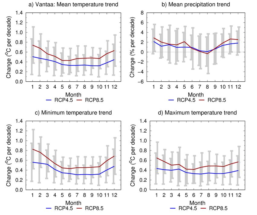
D6.4 Detailed report on local meteorological conditions

Project Acronym and        iSCAPE - Improving the Smart Control of Air Pollution in Europe
Name

Grant Agreement            689954
Number

Document Type              Report

Document version &         V0.4                       WP6
WP No.

Document Title             Detailed report on local meteorological conditions

Main authors               Kirsti Jylhä, Carl Fortelius, Olli Saranko, Kimmo Ruosteenoja,
                           Silvana Di Sabatino, Erika Brattich

Partner in charge          Finnish Meteorological Institute (FMI)

Contributing partners      ARPA-ER, UNIBO

Release date               8.7.2019

The publication reflects the author’s views. The European Commission is not liable for any use
that may be made of the information contained therein.

Document Control Page

Short Description This report documents findings from Task 6.4.1 “Simulation of Climate
                  Change in test case EU Cities”. The report includes climate projections
                  for all iSCAPE target cities: Bologna, Bottrop, Dublin, Guilford, Hasselt
                  and Vantaa. The magnitudes of climatic changes in the six cities by the
                  year 2050 were derived from a large number of climate model
                  simulations. An atmosphere-surface interaction module was then used to
                  study climatic impacts of a “Passive Control System” (PCS) intervention
                  in one of the cities, Vantaa, in the current climate and in a projected future
                  climate. The intervention consisted of increasing the fraction of green
                  spaces and relatively sparsely built suburban-type land use at the
                  expense of more densely built commercial and industrial areas.

                                                                                             -1-
D6.4 Detailed report on local meteorological conditions

Review status   Action          Person                         Date

                Quality Check   Coordination Team

                Internal Review Stefan Greiving (TUDO)
                                Gopinath Kalaiarasan (UoS)

Distribution    Public

                                                                                     -2-
D6.4 Detailed report on local meteorological conditions

Revision history

Version      Date               Modified by                Comments

V0.1                            Kirsti Jylhä, Carl
                                Fortelius, Olli Saranko,
             13/5/2019          Kimmo Ruosteenoja,          The first draft.
                                Silvana Di Sabatino,
                                Erika Brattich

V0.2                            Kirsti Jylhä, Carl       Mainly linguistic modifications.
                                Fortelius, Olli Saranko,
             5/6/2019           Kimmo Ruosteenoja,
                                Silvana Di Sabatino,
                                Erika Brattich

V0.3                                                       Addressed a reviewer’s (Stefan Greiving)
             19/6/2019          The authors
                                                           comments

V0.4                                                       Addressed another reviewer’s (Gopinath
             8/7/2019           The authors
                                                           Kalaiarasan Stefan Greiving) comments

Statement of originality:
This deliverable contains original unpublished work except where clearly indicated otherwise. Acknowledgement of
previously published material and of the work of others has been made through appropriate citation, quotation or
both.

                                                                                                     -3-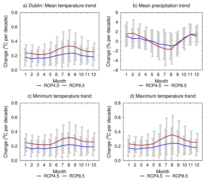
D6.4 Detailed report on local meteorological conditions

Table of Contents

Table of Contents
1      Executive Summary ........................................................................................... - 12 -
2      Introduction ........................................................................................................ - 14 -
3      Regional-scale climate projections for the iSCAPE cities ............................. - 16 -
    3.1    Material and methods ............................................................................................. - 16 -
      3.1.1   Representative Concentration Pathways .......................................................... - 16 -
      3.1.2   Global climate model simulations ...................................................................... - 17 -
      3.1.3   Construction of the climate change projections ................................................. - 18 -
    3.2    Results ..................................................................................................................... - 18 -
      3.2.1   Comparisons of the six iSCAPE cities ............................................................... - 19 -
      3.2.2   Climate change projections for Bologna ............................................................ - 26 -
      3.2.3   Climate change projections for Bottrop ............................................................. - 29 -
      3.2.4   Climate change projections for Dublin ............................................................... - 32 -
      3.2.5   Climate change projections for Guilford ............................................................ - 35 -
      3.2.6   Climate change projections for Hasselt ............................................................. - 38 -
      3.2.7   Climate change projections for Vantaa.............................................................. - 41 -
4      High-resolution simulations for Vantaa ........................................................... - 44 -
    4.1    SURFEX module and the intervention considered .............................................. - 44 -
    4.2    Methodological approach for the current climate ............................................... - 45 -
    4.3    Verification .............................................................................................................. - 46 -
    4.4    Methodological approach for the future climate ................................................. - 51 -
    4.5    Modelled impacts of climate change and green infrastructure.......................... - 53 -
      4.5.1    Impacts of climate change, current green spaces ............................................. - 53 -
      4.5.2    Impacts of the intervention in the present climate ............................................. - 56 -
      4.5.3    Impacts of the intervention under changing climate .......................................... - 58 -
    4.6    Summary and discussion of methods and results .............................................. - 61 -
5      Conclusions ....................................................................................................... - 62 -
6      References / Bibliography ................................................................................. - 64 -

                                                                                                                                         -4-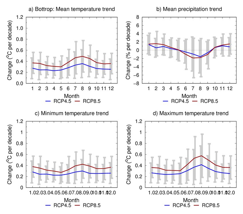
D6.4 Detailed report on local meteorological conditions

List of Tables
TABLE 1: CMIP5 GLOBAL CLIMATE MODELS USED IN CREATING CLIMATE CHANGE PROJECTIONS FOR THE ISCAPE
    CITIES. THE FIRST AND SECOND COLUMNS GIVE THE MODEL ACRONYM AND THE COUNTRY OF ORIGIN; THE EC-
    EARTH MODEL HAS BEEN DEVELOPED BY A CONSORTIUM OF SEVERAL EUROPEAN COUNTRIES. AN ASTERISK
    IN COLUMNS 3–10 INDICATES THAT DATA FROM THE CORRESPONDING MODEL WAS UTILIZED FOR A VARIABLE
    (TAVE: MEAN SURFACE AIR TEMPERATURE; TMIN: DAILY MINIMUM TEMPERATURE; TMAX: DAILY MAXIMUM
    TEMPERATURE; PREC: PRECIPITATION; SOLAR: INCIDENT SOLAR RADIATION AT THE SURFACE; PSL: SEA
    LEVEL PRESSURE; SPEED: SURFACE AIR WIND SPEED; DIR: WIND DIRECTION, STD: THE MONTHLY STANDARD
    DEVIATION OF THE TEMPORAL VARIABILITY OF DAILY MEAN TEMPERATURE). FOR FURTHER INFORMATION
    ABOUT THE INDIVIDUAL MODELS AND KEY REFERENCES, SEE TABLE 9.A.1 OF IPCC (2013). ...................- 17 -
TABLE 2: URBAN CHARACTERISTICS AT VANTAA TIKKURILA BEFORE AND AFTER THE INTERVENTION OF LOWER AND
    LESS DENSE BUILDINGS AND MORE WIDESPREAD GREEN SPACE. ...........................................................- 45 -
TABLE 3: THE MONTHS OF THE CLIMATOLOGICAL TEST REFERENCE YEAR FOR VANTAA (JYLHÄ ET AL., 2011)). - 45 -
TABLE 4: THE MEAN DIFFERENCES AND CORRELATION COEFFICIENTS, WITH P-VALUES, BETWEEN THE MODELLED
    TEST-YEAR DATA AND THE OBSERVED METEOROLOGICAL VARIABLES AT THE HELSINKI-VANTAA AIRPORT
    METEOROLOGICAL STATION. THE MEAN DIFFERENCES ARE CALCULATED USING THE DATA OF THE WHOLE
    TEST-YEAR. .......................................................................................................................................- 46 -

                                                                                                                                                      -5-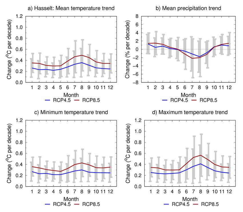
D6.4 Detailed report on local meteorological conditions

LIST OF FIGURES
FIGURE 1: TEMPORAL EVOLUTION OF THE GLOBAL ANTHROPOGENIC TOTAL EMISSIONS (LEFT: PGC/YR) AND
     ATMOSPHERIC ABUNDANCE (RIGHT: PARTS PER MILLION IN VOLUME) OF CARBON DIOXIDE IN 2000–2100
     ACCORDING TO FOUR RCP SCENARIOS; SEE THE LEGEND (BASED ON IPCC, 2013). PAST CARBON EMISSIONS
     (1980-2017) FROM FOSSIL FUEL COMBUSTION, INDUSTRIAL PROCESSES AND LAND-USE CHANGES ARE
     EXTRACTED FROM GLOBAL CARBON PROJECT (2018; HTTPS://WWW.ICOS-CP.EU/GCP/2018). THE
     OBSERVED ABUNDANCE DATA ARE AVAILABLE FOR DOWNLOAD FROM NOAA/ESRL. FOR THE ABUNDANCES
     OF OTHER WELL-MIXED GHGS AND AEROSOLS, SEE ANNEX II OF IPCC (2013). ....................................- 16 -
FIGURE 2: PROJECTED TEMPORAL EVOLUTION OF CHANGES IN 30-YEAR AVERAGES OF (A) ANNUAL MEAN
     TEMPERATURE, (B) ANNUAL MEAN DIURNAL TEMPERATURE RANGE, (C) ANNUAL PRECIPITATION, (D) ANNUAL
     MEAN SOLAR RADIATION FLUX AND (E) ANNUAL MEAN WIND SPEED IN THE SIX ISCAPE CITIES (SEE THE
     LEGEND) UNDER THE RCP8.5 SCENARIO. ............................................................................................- 20 -
FIGURE 3: PROJECTED TRENDS IN (A) MONTHLY MEAN AIR TEMPERATURE, (B) MONTHLY MEAN DIURNAL
     TEMPERATURE RANGE, AND (C) MONTHLY STANDARD DEVIATION OF THE TEMPORAL VARIABILITY OF DAILY
     MEAN TEMPERATURE BETWEEN THE BASELINE PERIOD AND 2040-2069 IN THE SIX CITIES (SEE THE LEGEND)
     UNDER THE RCP8.5 SCENARIO. THE MULTI-MODEL MEAN PROJECTIONS FOR EACH CALENDAR MONTH
     (1=JANUARY, 12=DECEMBER) ARE SHOWN. THE BASELINE PERIOD IS 1981-2010 IN (A-B) AND 1971-2000 IN
     (C). ...................................................................................................................................................- 21 -
FIGURE 4: PROJECTED TRENDS IN (A) MONTHLY PRECIPITATION TOTAL, (B) MONTHLY MEAN INCIDENT SOLAR
     RADIATION, AND (C) MONTHLY MEAN WIND SPEED BETWEEN THE PERIODS 1981-2010 AND 2040-2069 IN THE
     SIX CITIES (SEE THE LEGEND) UNDER THE RCP8.5 SCENARIO. THE MULTI-MODEL MEAN PROJECTIONS FOR
     EACH CALENDAR MONTH (1=JANUARY, 12=DECEMBER) ARE SHOWN. ...................................................- 22 -
FIGURE 5: SCATTER DIAGRAMS SHOWING THE SIMULATED MULTI-MODEL MEAN TRENDS BY THE 2050S IN
     TEMPERATURE, IN CONJUNCTION WITH CHANGES IN (A-B) PRECIPITATION, (C-D) INCIDENT SOLAR RADIATION
     AND (E-F) DIURNAL TEMPERATURE RANGE IN THE ISCAPE CITIES IN WINTER (LEFT) AND SUMMER (RIGHT)
     UNDER FOUR RCP GREENHOUSE GAS SCENARIOS. ..............................................................................- 23 -
FIGURE 6: SCATTER DIAGRAMS SHOWING THE SIMULATED MULTI-MODEL MEAN TRENDS BY THE 2050S IN INCIDENT
     SOLAR RADIATION, IN CONJUNCTION WITH CHANGES IN (A-B) DIURNAL TEMPERATURE RANGE AND (C-D)
     PRECIPITATION IN THE ISCAPE CITIES IN WINTER (LEFT) AND SUMMER (RIGHT) UNDER FOUR RCP
     GREENHOUSE GAS SCENARIOS. ..........................................................................................................- 24 -
FIGURE 7: PROJECTED CHANGES IN THE FREQUENCY DISTRIBUTIONS OF SIMULATED WIND DIRECTIONS IN (A)
     WINTER (DJF), (B) SPRING (MAM), (C) SUMMER (JJA) AND (D) AUTUMN BETWEEN THE PERIODS 1971-2000
     AND 2040-2069 IN THE SIX CITIES (SEE THE LEGEND) UNDER THE RCP8.5 SCENARIO. THE MULTI-MODEL
       MEAN PROJECTIONS FOR EACH CARDINAL AND INTERCARDINAL DIRECTION ARE GIVEN IN PERCENTAGE
       POINTS. TO GET A TREND AS A CHANGE IN PERCENTAGE POINTS PER DECADE, DIVIDE THE VALUES BY SEVEN. -
    25 -
FIGURE 8: PROJECTED TRENDS IN (A) MONTHLY MEAN AIR TEMPERATURE, (B) MONTHLY PRECIPITATION TOTAL, (C)
    MONTHLY MEAN OF DAILY MINIMUM TEMPERATURE, AND (D) MONTHLY MEAN OF DAILY MAXIMUM
    TEMPERATURE BETWEEN THE PERIODS 1981-2010 AND 2040-2069 IN BOLOGNA UNDER THE RCP4.5 AND
    RCP8.5 SCENARIOS. THE MULTI-MODEL MEAN PROJECTIONS FOR EACH CALENDAR MONTH (1 = JANUARY, 12
    = DECEMBER) ARE DEPICTED BY SOLID CURVES (BLUE FOR RCP4.5 AND RED FOR RCP8.5). THE GREY BARS
    INDICATE THE 90 % UNCERTAINTY INTERVALS FOR THE CHANGE (LEFT FOR RCP4.5 AND RIGHT FOR
    RCP8.5). ..........................................................................................................................................- 26 -
FIGURE 9: PROJECTED TRENDS IN (A) MONTHLY MEAN DIURNAL TEMPERATURE RANGE, (B) MONTHLY MEAN
    INCIDENT SOLAR RADIATION, AND (C) MONTHLY STANDARD DEVIATION OF THE TEMPORAL VARIABILITY OF
    DAILY MEAN TEMPERATURE BY THE PERIOD 2040–2069 IN BOLOGNA UNDER THE RCP4.5 AND RCP8.5
    SCENARIOS. THE BASELINE PERIOD IS 1981-2010 (TOP) OR 1971-2000 (BOTTOM). FOR FURTHER
    INFORMATION, SEE THE CAPTION FOR FIGURE 8. ..................................................................................- 27 -
FIGURE 10: PROJECTED TRENDS IN A) MONTHLY MEAN SURFACE AIR PRESSURE AND B) WIND SPEED BETWEEN THE
    PERIODS 1981-2010 AND 2040-2069 IN BOLOGNA UNDER THE RCP4.5 (BLUE) AND RCP8.5 (RED)
    SCENARIOS. FOR FURTHER INFORMATION, SEE THE CAPTION FOR FIGURE 8. .........................................- 28 -
FIGURE 11. PROJECTED MULTI-MODEL MEAN CHANGES IN THE FREQUENCY DISTRIBUTIONS OF SIMULATED WIND
    DIRECTIONS IN WINTER (DJF), SPRING (MAM), SUMMER (JJA) AND AUTUMN BETWEEN THE PERIODS 1971-
    2000 AND 2040-2069 IN BOLOGNA UNDER THE RCP8.5 SCENARIO. THE CHANGES ARE GIVEN IN
                                                                                                                                                            -6-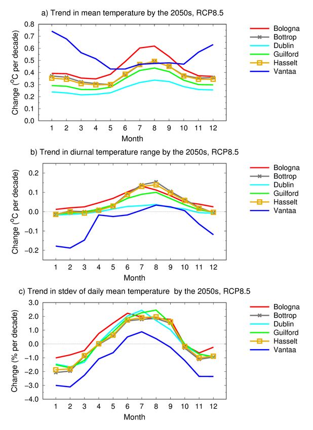
D6.4 Detailed report on local meteorological conditions

       PERCENTAGE POINTS, WITH RED BARS DEPICTING AN INCREASE AND BLUE BARS A DECREASE IN THE
       FREQUENCY. THE CIRCLES INDICATE THE SCALE OF CHANGES FOR EACH CARDINAL AND INTERCARDINAL
    DIRECTION WITH AN INTERVAL OF 0.5%. ..............................................................................................- 28 -
FIGURE 12: PROJECTED TRENDS IN (A) MONTHLY MEAN AIR TEMPERATURE, (B) MONTHLY PRECIPITATION TOTAL,
    (C) MONTHLY MEAN OF DAILY MINIMUM TEMPERATURE, AND (D) MONTHLY MEAN OF DAILY MAXIMUM
    TEMPERATURE BETWEEN THE PERIODS 1981-2010 AND 2040-2069 IN BOTTROP UNDER THE RCP4.5 AND
    RCP8.5 SCENARIOS. THE MULTI-MODEL MEAN PROJECTIONS FOR EACH CALENDAR MONTH (1 = JANUARY, 12
    = DECEMBER) ARE DEPICTED BY SOLID CURVES (BLUE FOR RCP4.5 AND RED FOR RCP8.5). THE GREY BARS
    INDICATE THE 90 % UNCERTAINTY INTERVALS FOR THE CHANGE (LEFT FOR RCP4.5 AND RIGHT FOR
    RCP8.5). ..........................................................................................................................................- 29 -
FIGURE 13: PROJECTED TRENDS IN (A) MONTHLY MEAN DIURNAL TEMPERATURE RANGE, (B) MONTHLY MEAN
    INCIDENT SOLAR RADIATION, AND (C) MONTHLY STANDARD DEVIATION OF THE TEMPORAL VARIABILITY OF
    DAILY MEAN TEMPERATURE BY THE PERIOD 2040–2069 IN BOTTROP UNDER THE RCP4.5 (BLUE) AND
    RCP8.5 (RED) SCENARIOS. THE BASELINE PERIOD IS 1981-2010 (TOP) OR 1971-2000 (BOTTOM). FOR
    FURTHER INFORMATION, SEE THE CAPTION FOR FIGURE 12. .................................................................- 30 -
FIGURE 14: PROJECTED TRENDS IN A) MONTHLY MEAN SURFACE AIR PRESSURE AND B) WIND SPEED BETWEEN THE
    PERIODS 1981-2010 AND 2040-2069 IN BOTTROP UNDER THE RCP4.5 (BLUE) AND RCP8.5 (RED)
    SCENARIOS. FOR FURTHER INFORMATION, SEE CAPTION FOR FIGURE 12. ..............................................- 31 -
FIGURE 15. PROJECTED MULTI-MODEL MEAN CHANGES IN THE FREQUENCY DISTRIBUTIONS OF SIMULATED WIND
    DIRECTIONS IN WINTER (DJF), SPRING (MAM), SUMMER (JJA) AND AUTUMN BETWEEN THE PERIODS 1971-
    2000 AND 2040-2069 IN BOTTROP UNDER THE RCP8.5 SCENARIO. THE CHANGES ARE GIVEN IN
    PERCENTAGE POINTS, WITH RED BARS DEPICTING AN INCREASE AND BLUE BARS A DECREASE IN THE
    FREQUENCY. THE CIRCLES INDICATE THE SCALE OF CHANGES FOR EACH CARDINAL AND INTERCARDINAL
    DIRECTION WITH AN INTERVAL OF 0.5%. ..............................................................................................- 31 -
FIGURE 16: PROJECTED TRENDS IN (A) MONTHLY MEAN AIR TEMPERATURE, (B) MONTHLY PRECIPITATION TOTAL,
    (C) MONTHLY MEAN OF DAILY MINIMUM TEMPERATURE, AND (D) MONTHLY MEAN OF DAILY MAXIMUM
    TEMPERATURE BETWEEN THE PERIODS 1981-2010 AND 2040-2069 IN DUBLIN UNDER THE RCP4.5 AND
    RCP8.5 SCENARIOS. THE MULTI-MODEL MEAN PROJECTIONS FOR EACH CALENDAR MONTH (1 = JANUARY, 12
    = DECEMBER) ARE DEPICTED BY SOLID CURVES (BLUE FOR RCP4.5 AND RED FOR RCP8.5). THE GREY BARS
    INDICATE THE 90 % UNCERTAINTY INTERVALS FOR THE CHANGE (LEFT FOR RCP4.5 AND RIGHT FOR
    RCP8.5). ..........................................................................................................................................- 32 -
FIGURE 17: PROJECTED TRENDS IN (A) MONTHLY MEAN DIURNAL TEMPERATURE RANGE, (B) MONTHLY MEAN
    INCIDENT SOLAR RADIATION, AND (C) MONTHLY STANDARD DEVIATION OF THE TEMPORAL VARIABILITY OF
    DAILY MEAN TEMPERATURE BY THE PERIOD 2040–2069 IN DUBLIN UNDER THE RCP4.5 (BLUE) AND RCP8.5
    (RED) SCENARIOS. THE BASELINE PERIOD IS 1981-2010 (TOP) OR 1971-2000 (BOTTOM). FOR FURTHER
    INFORMATION, SEE THE CAPTION FOR FIGURE 16. ................................................................................- 33 -
FIGURE 18: PROJECTED TRENDS IN A) MONTHLY MEAN SURFACE AIR PRESSURE AND B) WIND SPEED BETWEEN THE
    PERIODS 1981-2010 AND 2040-2069 IN DUBLIN UNDER THE RCP4.5 (BLUE) AND RCP8.5 (RED)
    SCENARIOS. FOR FURTHER INFORMATION, SEE CAPTION FOR FIGURE 16 ...............................................- 34 -
FIGURE 19: PROJECTED MULTI-MODEL MEAN CHANGES IN THE FREQUENCY DISTRIBUTIONS OF SIMULATED WIND
    DIRECTIONS IN WINTER (DJF), SPRING (MAM), SUMMER (JJA) AND AUTUMN BETWEEN THE PERIODS 1971-
    2000 AND 2040-2069 IN DUBLIN UNDER THE RCP8.5 SCENARIO. THE CHANGES ARE GIVEN IN PERCENTAGE
    POINTS, WITH RED BARS DEPICTING AN INCREASE AND BLUE BARS A DECREASE IN THE FREQUENCY. THE
       CIRCLES INDICATE THE SCALE OF CHANGES FOR EACH CARDINAL AND INTERCARDINAL DIRECTION WITH AN
    INTERVAL OF 0.5%. ............................................................................................................................- 34 -
FIGURE 20: PROJECTED TRENDS IN (A) MONTHLY MEAN AIR TEMPERATURE, (B) MONTHLY PRECIPITATION TOTAL,
    (C) MONTHLY MEAN OF DAILY MINIMUM TEMPERATURE, AND (D) MONTHLY MEAN OF DAILY MAXIMUM
    TEMPERATURE BETWEEN THE PERIODS 1981-2010 AND 2040-2069 IN GUILFORD UNDER THE RCP4.5 AND
    RCP8.5 SCENARIOS. THE MULTI-MODEL MEAN PROJECTIONS FOR EACH CALENDAR MONTH (1 = JANUARY, 12
    = DECEMBER) ARE DEPICTED BY SOLID CURVES (BLUE FOR RCP4.5 AND RED FOR RCP8.5). THE GREY BARS
    INDICATE THE 90 % UNCERTAINTY INTERVALS FOR THE CHANGE (LEFT FOR RCP4.5 AND RIGHT FOR
    RCP8.5). ..........................................................................................................................................- 35 -
FIGURE 21: PROJECTED TRENDS IN (A) MONTHLY MEAN DIURNAL TEMPERATURE RANGE, (B) MONTHLY MEAN
    INCIDENT SOLAR RADIATION, AND (C) MONTHLY STANDARD DEVIATION OF THE TEMPORAL VARIABILITY OF
    DAILY MEAN TEMPERATURE BY THE PERIOD 2040–2069 IN GUILFORD UNDER THE RCP4.5 (BLUE) AND

                                                                                                                                                       -7-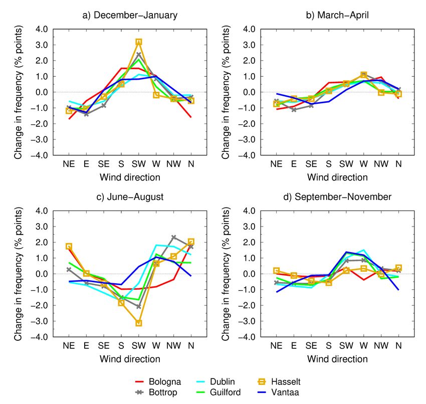
D6.4 Detailed report on local meteorological conditions
RCP8.5 (RED) SCENARIOS. THE BASELINE PERIOD IS 1981-2010 (TOP) OR 1971-2000 (BOTTOM). FOR
FURTHER INFORMATION, SEE THE CAPTION FOR FIGURE 20. .................................................................- 36 -
FIGURE 22: PROJECTED TRENDS IN A) MONTHLY MEAN SURFACE AIR PRESSURE AND B) WIND SPEED BETWEEN THE
PERIODS 1981-2010 AND 2040-2069 IN GUILFORD UNDER THE RCP4.5 (BLUE) AND RCP8.5 (RED)
SCENARIOS. FOR FURTHER INFORMATION, SEE CAPTION FOR FIGURE 20. ..............................................- 37 -
FIGURE 23: PROJECTED MULTI-MODEL MEAN CHANGES IN THE FREQUENCY DISTRIBUTIONS OF SIMULATED WIND
DIRECTIONS IN WINTER (DJF), SPRING (MAM), SUMMER (JJA) AND AUTUMN BETWEEN THE PERIODS 1971-
2000 AND 2040-2069 IN GUILFORD UNDER THE RCP8.5 SCENARIO. THE CHANGES ARE PROVIDED IN
PERCENTAGE POINTS, WITH RED BARS DEPICTING AN INCREASE AND BLUE BARS A DECREASE IN THE
FREQUENCY. THE CIRCLES INDICATE THE SCALE OF CHANGES FOR EACH CARDINAL AND INTERCARDINAL
DIRECTION WITH AN INTERVAL OF 0.5%. ..............................................................................................- 37 -
FIGURE 24: PROJECTED TRENDS IN (A) MONTHLY MEAN AIR TEMPERATURE, (B) MONTHLY PRECIPITATION TOTAL,
(C) MONTHLY MEAN OF DAILY MINIMUM TEMPERATURE, AND (D) MONTHLY MEAN OF DAILY MAXIMUM
TEMPERATURE BETWEEN THE PERIODS 1981-2010 AND 2040-2069 IN HASSELT UNDER THE RCP4.5 AND
RCP8.5 SCENARIOS. THE MULTI-MODEL MEAN PROJECTIONS FOR EACH CALENDAR MONTH (1 = JANUARY, 12
= DECEMBER) ARE DEPICTED BY SOLID CURVES (BLUE FOR RCP4.5 AND RED FOR RCP8.5). THE GREY BARS
INDICATE THE 90 % UNCERTAINTY INTERVALS FOR THE CHANGE (LEFT FOR RCP4.5 AND RIGHT FOR
RCP8.5). ..........................................................................................................................................- 38 -
FIGURE 25: PROJECTED TRENDS IN (A) MONTHLY MEAN DIURNAL TEMPERATURE RANGE, (B) MONTHLY MEAN
INCIDENT SOLAR RADIATION, AND (C) MONTHLY STANDARD DEVIATION OF THE TEMPORAL VARIABILITY OF
DAILY MEAN TEMPERATURE BY THE PERIOD 2040–2069 IN HASSELT UNDER THE RCP4.5 (BLUE) AND
RCP8.5 (RED) SCENARIOS. THE BASELINE PERIOD IS 1981-2010 (TOP) OR 1971-2000 (BOTTOM). FOR
FURTHER INFORMATION, SEE THE CAPTION FOR FIGURE 24. .................................................................- 39 -
FIGURE 26: PROJECTED TRENDS IN A) MONTHLY MEAN SURFACE AIR PRESSURE AND B) WIND SPEED BETWEEN THE
PERIODS 1981-2010 AND 2040-2069 IN HASSELT UNDER THE RCP4.5 (BLUE) AND RCP8.5 (RED)
SCENARIOS. FOR FURTHER INFORMATION, SEE CAPTION FOR FIGURE 24. ..............................................- 40 -
FIGURE 27: PROJECTED MULTI-MODEL MEAN CHANGES IN THE FREQUENCY DISTRIBUTIONS OF SIMULATED WIND
DIRECTIONS IN WINTER (DJF), SPRING (MAM), SUMMER (JJA) AND AUTUMN BETWEEN THE PERIODS 1971-
2000 AND 2040-2069 IN HASSELT UNDER THE RCP8.5 SCENARIO. THE CHANGES ARE PROVIDED IN
PERCENTAGE POINTS, WITH RED BARS DEPICTING AN INCREASE AND BLUE BARS A DECREASE IN THE
FREQUENCY. THE CIRCLES INDICATE THE SCALE OF CHANGES FOR EACH CARDINAL AND INTERCARDINAL
DIRECTION WITH AN INTERVAL OF 0.5%. ..............................................................................................- 40 -
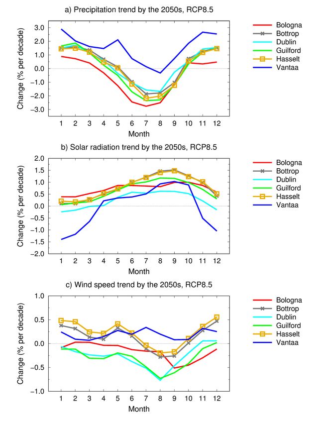
FIGURE 28: PROJECTED TRENDS IN (A) MONTHLY MEAN AIR TEMPERATURE, (B) MONTHLY PRECIPITATION TOTAL,
(C) MONTHLY MEAN OF DAILY MINIMUM TEMPERATURE, AND (D) MONTHLY MEAN OF DAILY MAXIMUM
TEMPERATURE BETWEEN THE PERIODS 1981-2010 AND 2040-2069 IN VANTAA UNDER THE RCP4.5 AND
RCP8.5 SCENARIOS. THE MULTI-MODEL MEAN PROJECTIONS FOR EACH CALENDAR MONTH (1 = JANUARY, 12
= DECEMBER) ARE DEPICTED BY SOLID CURVES (BLUE FOR RCP4.5 AND RED FOR RCP8.5). THE GREY BARS
INDICATE THE 90 % UNCERTAINTY INTERVALS FOR THE CHANGE (LEFT FOR RCP4.5 AND RIGHT FOR
RCP8.5). ..........................................................................................................................................- 41 -
FIGURE 29: PROJECTED TRENDS IN (A) MONTHLY MEAN DIURNAL TEMPERATURE RANGE, (B) MONTHLY MEAN
INCIDENT SOLAR RADIATION, AND (C) MONTHLY STANDARD DEVIATION OF THE TEMPORAL VARIABILITY OF
DAILY MEAN TEMPERATURE BY THE PERIOD 2040–2069 IN VANTAA UNDER THE RCP4.5 (BLUE) AND RCP8.5
(RED) SCENARIOS. THE BASELINE PERIOD IS 1981-2010 (TOP) OR 1971-2000 (BOTTOM). FOR FURTHER
INFORMATION, SEE THE CAPTION FOR FIGURE 28. ................................................................................- 42 -
FIGURE 30: PROJECTED TRENDS IN A) MONTHLY MEAN SURFACE AIR PRESSURE AND B) WIND SPEED BETWEEN THE
PERIODS 1981-2010 AND 2040-2069 IN VANTAA UNDER THE RCP4.5 (BLUE) AND RCP8.5 (RED)
SCENARIOS. FOR FURTHER INFORMATION, SEE CAPTION FOR FIGURE 28. ..............................................- 43 -
FIGURE 31: PROJECTED MULTI-MODEL MEAN CHANGES IN THE FREQUENCY DISTRIBUTIONS OF SIMULATED WIND
DIRECTIONS IN WINTER (DJF), SPRING (MAM), SUMMER (JJA) AND AUTUMN BETWEEN THE PERIODS 1971-
2000 AND 2040-2069 IN VANTAA UNDER THE RCP8.5 SCENARIO. THE CHANGES ARE PROVIDED IN
PERCENTAGE POINTS, WITH RED BARS DEPICTING AN INCREASE AND BLUE BARS A DECREASE IN THE
FREQUENCY. THE CIRCLES INDICATE THE SCALE OF CHANGES FOR EACH CARDINAL AND INTERCARDINAL
DIRECTION WITH AN INTERVAL OF 0.5%. ..............................................................................................- 43 -
FIGURE 32: URBAN LAND USE TYPES OVER THE DOMAIN OF SURFEX. SUBURBAN TYPES ARE SHOWN IN GREY,
COMMERCIAL AND INDUSTRIAL AREAS IN RED, PARKS AND SPORTS FACILITIES IN GREEN, AND AIRPORTS AND
-8-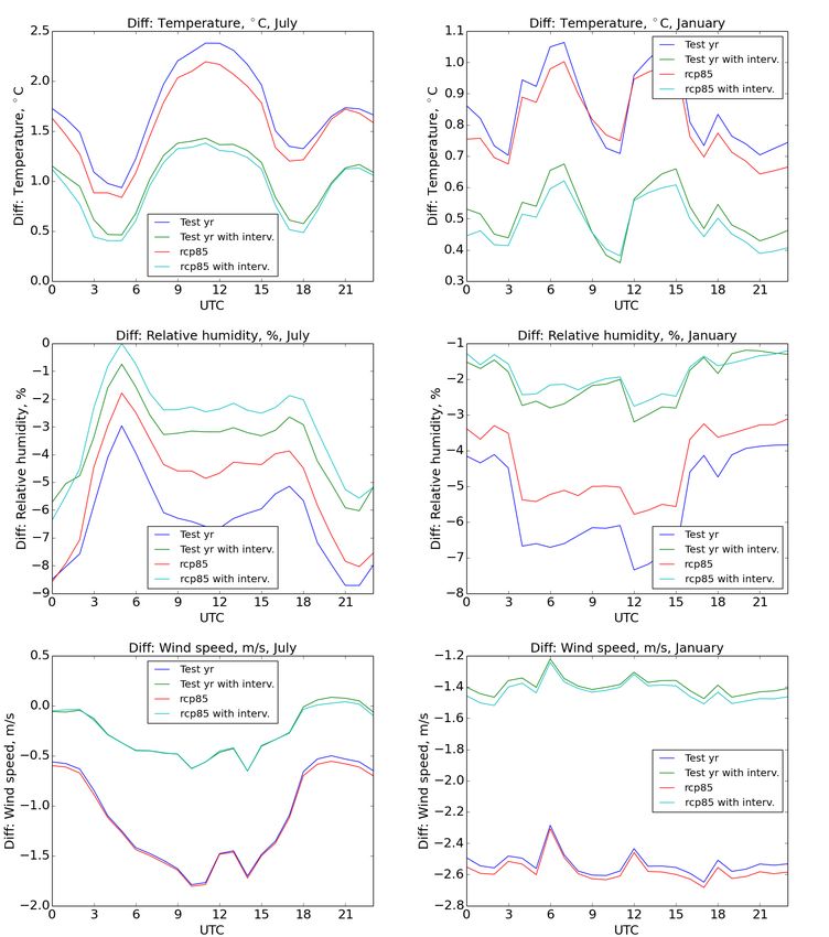
D6.4 Detailed report on local meteorological conditions

       PORTS IN BLUE COLOR. THE COMMERCIAL AREA OF VANTAA TIKKURILA AND THE FOREST OF THE
    SIPOONKORPI NATIONAL PARK ARE SHOWN BY BLACK AND GREEN STARS, RESPECTIVELY. .....................- 44 -
FIGURE 33. OBSERVED AND MODELLED SEASONAL MEAN DIURNAL TEMPERATURE CYCLES AT THE HELSINKI
    VANTAA AIRPORT FOR THE TEST YEAR. NOTE THE DIFFERENT VERTICAL SCALES IN THE DIAGRAMS. ........- 47 -
FIGURE 34: OBSERVED AND MODELLED SEASONAL MEAN DIURNAL CYCLES OF RELATIVE HUMIDITY AT THE HELSINKI
    VANTAA AIRPORT FOR THE TEST-YEAR. ...............................................................................................- 48 -
FIGURE 35: OBSERVED AND MODELLED SEASONAL MEAN DIURNAL CYCLES OF WIND SPEED AT HELSINKI VANTAA
    AIRPORT FOR THE TEST-YEAR. ............................................................................................................- 49 -
FIGURE 36: OBSERVED AND MODELLED 12-HOURLY PRECIPITATION TOTALS FOR THE TEST-YEAR. ..................- 49 -
FIGURE 37: OBSERVED AND MODELLED MONTHLY PRECIPITATION TOTALS FOR THE TEST-YEAR. .....................- 50 -
FIGURE 38: MONTHLY AVERAGED METEOROLOGICAL FORCING EXTRACTED FROM THE SIMULATED DATA FOR THE
    HELSINKI-VANTAA AIRPORT. BLUE: AS GIVEN BY HARMONIE DURING THE TEST-YEAR. RED: AS
    INCREMENTED TO REPRESENT THE MID-2050S CLIMATE ACCORDING TO RCP8.5. PANELS FROM TOP LEFT TO
    BOTTOM RIGHT SHOW, RESPECTIVELY AIR TEMPERATURE, RELATIVE HUMIDITY, INSOLATION, DOWNWELLING
    TERRESTRIAL RADIATION, WIND SPEED, AND PRECIPITATION AMOUNT. TEMPERATURE, HUMIDITY, AND WIND
    SPEED REPRESENT CONDITIONS AT 12 M ABOVE GROUND. ....................................................................- 52 -
FIGURE 39: MONTHLY MEAN AIR TEMPERATURE (TOP), RELATIVE HUMIDITY (MIDDLE) AND WIND SPEED (BOTTOM)
    AS SIMULATED BY SURFEX IN JULY. CONDITIONS OF THE TEST-YEAR, REPRESENTING CURRENT CLIMATE,
    ARE SHOWN ON THE LEFT. THE HIGH-RESOLUTION CHANGES INDUCED BY THE ALTERED FORCING, I.E.,
    REGIONAL-SCALE CLIMATE CHANGE, ARE SHOWN ON THE RIGHT. THE COMMERCIAL AREA OF VANTAA
    TIKKURILA AND THE FOREST OF THE SIPOONKORPI NATIONAL PARK ARE SHOWN BY BLACK AND GREEN
    STARS, RESPECTIVELY. ......................................................................................................................- 54 -
FIGURE 40: AS FIGURE 39, BUT FOR THE MONTH OF JANUARY......................................................................- 55 -
FIGURE 41: SCATTER PLOTS OF AIR TEMPERATURE (TOP PANELS), RELATIVE HUMIDITY (MIDDLE PANELS) AND WIND
    SPEED (BOTTOM PANELS), SHOWING THE RESPONSE TO CHANGING THE URBAN LAYOUT IN SURFEX FOR
    TIKKURILA IN VANTAA IN JULY (LEFT HAND COLUMN) AND JANUARY (RIGHT HAND COLUMN).....................- 57 -
FIGURE 42: MONTHLY MEAN DIURNAL CYCLES OF AIR TEMPERATURE (TOP PANELS), RELATIVE HUMIDITY (MIDDLE
    PANELS) AND WIND SPEED (BOTTOM PANELS), SHOWING THE RESPONSE TO CHANGING CLIMATE AND URBAN
    LAYOUT IN SURFEX FOR TIKKURILA IN VANTAA IN THE MONTHS OF JULY (LEFT HAND COLUMN) AND JANUARY
    (RIGHT HAND COLUMN). LOCAL MIDDAY OCCURS AT ABOUT 10 UTC. NOTE THE DIFFERENT SCALES ON THE Y-
    AXES. ................................................................................................................................................- 59 -
FIGURE 43: MONTHLY MEAN DIURNAL CYCLES OF DIFFERENCE BETWEEN VANTAA TIKKURILA AND THE
    SIPOONKORPI NATIONAL PARK FOR AIR TEMPERATURE (TOP PANELS), RELATIVE HUMIDITY (MIDDLE PANELS)
    AND WIND SPEED (BOTTOM PANELS), SHOWING THE RESPONSE TO CHANGING CLIMATE AND URBAN LAYOUT IN
    SURFEX FOR TIKKURILA IN VANTAA IN THE MONTHS OF JULY (LEFT HAND COLUMN) AND JANUARY (RIGHT
    HAND COLUMN). LOCAL MIDDAY OCCURS AT ABOUT 10 UTC. NOTE THE DIFFERENT SCALES ON THE Y-AXES.. -
    60 -

                                                                                                                                                          -9-
D6.4 Detailed report on local meteorological conditions
List of abbreviations
CC: Climate change
CMIP: Coupled Model Intercomparison Project
CO2: Carbon Dioxide
D: Deliverable
Dir: Wind Direction
EU: European Union
GCM: Global Climate Model
GHG: Greenhouse gas
IPCC: Intergovernmental Panel on Climate Change
PCS: Passive Control System
Prec: Precipitation
PSL: sea level pressure
RCP: Representative Concentration Pathway
RCP2.6: Low RCP in which GHG emissions are substantially reduced, leading to a
radiative forcing of 2.6 W m-2 in the year 2100
RCP4.5: Medium-Low RCP in which the radiative forcing is stabilized at 4.5 W m-2 in
2100 without ever exceeding that value
RCP6.0: Medium-High RCP leading to a radiative forcing of 6.0 W m-2 in 2100.
RCP8.5: High RCP in which GHG emissions and concentrations increase
considerably over time, leading to a radiative forcing of 8.5 W m-2 in 2100.
Solar: incident solar radiation at the surface
Speed surface air wind speed
STD: the monthly standard deviation of the temporal variability of daily mean
temperature
SURFEX: A system of physically-based numerical models of air-surface interactions
Tave: mean surface air temperature
Tmin: daily minimum temperature
Tmax: daily maximum temperature
UHI: Urban Heat Island
UNFCC: United Nations Framework Convention on Climate Change
WMO: World Meteorological Organization
WP: Work Package
- 10 -D6.4 Detailed report on local meteorological conditions
- 11 -D6.4 Detailed report on local meteorological conditions
1 Executive Summary
The purpose of this Deliverable is to document findings from Task 6.4.1 “Simulation of Climate
Change in test case EU Cities”. The task focused on climate projections for all iSCAPE target
cities: Bologna in Italy, Bottrop in Germany, Dublin in Ireland, Guilford in United Kingdom, Hasselt
in Belgium and Vantaa in Finland. By utilizing a large number of climate model simulations, the
magnitudes of climatic changes by the year 2050 were assessed for the six cities. An atmosphere-
surface interaction module was then used to study climatic impacts of a “Passive Control System”
(PCS) intervention in one of the cities, Vantaa, in the current climate and in a projected future
climate. The intervention consisted of increasing the fraction of green spaces and relatively
sparsely built suburban-type land use at the expense of more densely built commercial and
industrial areas.
The climate change assessments were grounded on simulations conducted with 28 CMIP5 global
climate models. The projected changes in the climates of the iSCAPE cities were found to have
several common features but also clear differences. Under a scenario of high global greenhouse
gas concentrations (RCP8.5), the projected warming is expected to increase almost linearly in
time during the course of the ongoing century, most rapidly in Vantaa in northern Europe and
slowest in Dublin in western central Europe. Apart from Vantaa, the projected annual mean
increases in daily maximum temperature are larger than those in the daily minima. The
climatological (30-year average) annual mean precipitation is projected to decrease in Bologna
and either increase or remain almost unaltered elsewhere. The annual total incident solar radiation
is projected to increase in all six cities, most strongly in Bottrop and Hasselt and least in Vantaa
and Dublin. A common feature for all the six iSCAPE cities is also that the projected changes do
not distribute evenly throughout the year. However, the annual cycles of the projected changes
the selected cities.
In more detail, the following changes in climate by 2050 were simulated for the test case EU cities:
• In Bologna, there is a general trend towards higher temperatures and more abundant solar
radiation, particularly so in summer; in addition, the projections indicate increases in diurnal
temperature range and day-to-day temperature variability during the warmer half of the
year, and reductions in summer precipitation. Minor decreases in mean wind speed might
occur in autumn and some turning of wind directions in summer and winter.
• The projected multi-model mean changes in temperature and precipitation in Bottrop
resemble those for Bologna but are in general weaker. In contrast, in summer and autumn
solar radiation is expected to increase even more strongly than in Bologna. The portion of
south-westerly winds might slightly increase in winter and decrease in summer.
• Among the six iSCAPE cities, the projected long-term trend of warming is weakest in
Dublin, both on annual and monthly bases. Also, the relative increase in annual insolation
is lower in Dublin than in most of the other iSCAPE cities. The same is true for increases
in diurnal temperature range in summer. Conversely, the projected percentage decreases
in summer precipitation and increases in day-to-day variability in daily mean temperatures
in summer are of the average magnitude, whereas the decreases in mean wind in summer
are slightly larger (or less minor), although with high uncertainty, than in most of the other
iSCAPE cities.
• The climate projections for Guilford resemble those for Dublin in several aspects, but the
changes are generally larger. The percentage increase in summertime diurnal temperature
range is about twice as large as in Dublin, and the annual mean solar radiation flux is
- 12 -D6.4 Detailed report on local meteorological conditions
projected to increase approximately at the same rate as in Bologna, although not as rapidly
as in Bottrop and Hasselt.
• The climate projections for Hasselt are very similar to those for the adjacent iSCAPE city,
Bottrop. There is a general trend towards higher temperatures, particularly so in summer,
slightly wetter winters and drier summers, more solar radiation and little changes in mean
wind speed. The multi-model mean projections show slight increases (decreases) in the
portion of south-westerly winds in winter (summer).
• The projected future changes in the climate of Vantaa in northern Europe deviate from
those for the other iSCAPE cities. There is a general trend towards higher temperatures,
but unlike in the other cities, the trend is stronger in winter than in summer. Also, the
projected changes in precipitation and solar radiation are more pronounced in winter than
in summer. In accordance with the other cities, the multi-model mean changes in the mean
wind speed are small compared to the uncertainty ranges.
The test iSCAPE cities are well spread over the European latitudinal bands and represent different
climate zones. The climate projections given here are well representative of the future climate
change that will impact Europe and might thus be extended to other European cities.
In order to assess the impacts of the proposed passive control system (PCS), i.e. green
infrastructure in this case, the air-surface interaction module SURFEX was used for the test case
EU City Vantaa. The characteristics of the city-block, and the presence and properties of gardens
and parks were taken into account in the simulations. The radiative and thermal properties of the
building materials, as well as anthropogenic sources of heat and moisture from traffic and industry
and civil buildings were likewise considered. Using specific procedures together with the CMIP5
model simulation data and the SURFEX model, future scenario weather data for Vantaa were
developed at a very high temporal and spatial resolution. In these simulations, the presence of the
built-up areas strongly modulates local climate, and differences between the town and the
surrounding forested areas were found to remain similar to the present ones also in the 2050s.
After validation with weather observations, SURFEX was applied to explore the consequences of
altering the urban layout by replacing relatively densely built commercial and industrial areas with
a suburban-type land use featuring lower and less dense buildings and more widespread
vegetated areas. For the city of Vantaa, this PCS intervention did not involve a dramatic change
in the urban characteristics, and, accordingly the effect observed in the simulation outputs was
rather modest. The strongest influence was found in wind speed
Comparing the results for the recent past climate and the mid-2050s, it was found that climate
warming at street level was only slightly reduced by the simulated changes in urban morphology.
By contrast, changes in morphology had an important or even dominating effect in terms of relative
humidity and wind speed, compared with the projected changes in climate.
Based on urban development models considered in iSCAPE Deliverable 1.2 (‘Guidelines to
promote passive methods for improving urban air quality in climate change scenarios’1), Vantaa
can be classified as a decentralised city with no dominant core city and no clear distinction
between open spaces and built-up areas. Over 60% of its area is currently green spaces and
water bodies contrasting only 18% of sealed air- and watertight ground surface. The classification
for Vantaa differs from that of the other iSCAPE cities, as Bologna and Dublin are examples of a
compact city, and Bottrop, Guilford and Hasselt are examples of a decentralised concentration. In
1 The report is available at the iSCAPE results webpage
- 13 -D6.4 Detailed report on local meteorological conditions
addition, the current climate and the climate change projections for the city of Vantaa in northern
Europe deviate from those for the other iSCAPE cities. Therefore the SURFEX model results for
Vantaa, consisting of very high-resolution future scenario weather data and assessments of the
PCS impacts, cannot be directly extended to the other European cities. However, the methodology
could be applied for any urban areas with adequate resources.
2 Introduction
The iSCAPE project (Improving the Smart Control of Air Pollution in Europe) works on integrating
and advancing the control of air quality and carbon emissions in European cities in the changing
climate. iSCAPE focuses on the use of “Passive Control Systems” (PCSs) in urban spaces, on
policy intervention and behavioural changes of citizens lifestyle. The target cities are Bologna in
Italy, Bottrop in Germany, Dublin in Ireland, Guilford in United Kingdom, Hasselt in Belgium and
Vantaa in Finland. Infrastructural PCSs in the iSCAPE cities include low boundary walls (Dublin),
photocatalytic coatings (Lazzaretto in the outskirts of Bologna), urban design and planning
(Bottrop) and various green infrastructures: hedge-rows (Guilford), trees (Bologna) and green
urban spaces (Vantaa). For a review of the characteristics, strengths and limitations of PCSs, the
reader is referred to D1.2.
WP6 of the iSCAPE project aims to quantify the impacts of the infrastructural PCSs with respect
to air pollutants levels and their linkages to climate changes in the urban environment. The
objective is to evaluate their effectiveness both in the current climate and under future scenarios
around the year 2050. Based on a review of previous research (D1.2) as well as on the results of
the current project2, climatic and meteorological factors influence the efficiency of the PCSs at
various scales. For example, the impact of trees on pollutant exposure depends, among others,
on meteorological conditions (wind, turbulence) (D5.2 and D6.2). Furthermore, the air purification
efficiency of photocatalytic coatings partly depends on climatic factors, such as relative humidity,
solar radiation and temperature, and thereby on their changes in the future (D3.6). On the other
hand, urban green and blue spaces might have a cooling effect, moderating potential overheating
of cities relative to the countryside (urban heat island, UHI).
An overview of the latest understanding of climate and climate change and its connection with
urban air quality was provided in iSCAPE Deliverable D1.4 (Di Sabatino et al., 2017) that also
reviewed literature about the detected past and projected future climatic trends in broad iSCAPE
study regions. It likewise discussed climate change modelling and downscaling approaches and
presented preliminary comparisons between the iSCAPE study regions in terms of climate change
projections.
2 See the following reports that are or will be made available on the iSCAPE results webpage:
D3.6, ‘Report on photocatalytic coating’,
D3.8, ‘Report on deployment of neighbourhood level interventions’,
D5.2, ‘Air pollution and meteorology monitoring report’,
D5.3, ‘Report on interventions’,
D5.4, ‘Strategic portfolio choice’,
D6.2, ‘Microscale CFD evaluation of PCSs impacts on air quality’,
D6.3, ‘Detailed report based on numerical simulations of the effect of PCS at the urban level’,
D6.5, ‘Detailed report of the effect of PCSs on air quality in the future CC (2050) in the target
cities’.
- 14 -D6.4 Detailed report on local meteorological conditions
The current report documents findings from Task 6.4.1 “Simulation of Climate Change in test case
EU Cities”. The report is organized in two main parts. First, regional scale climate projections by
the year 2050, derived from a large number of climate model simulations, are presented for all the
six iSCAPE cities. Second, using an atmosphere-surface interaction module, climatic influences
of green infrastructure are assessed for one of the cities, Vantaa in northern Europe, both in the
current climate and in a projected future climate. The latter part discusses meteorological model
simulations with a high temporal and spatial resolution; in principle such simulations could be
conducted for any urban areas.
Previously, in D1.4 Di Sabatino et al. (2017) highlighted three different climatological variables of
the highest relevance in the context of air pollutants: surface air temperature, precipitation and
sea level pressure. For example, increasing temperatures and decreasing precipitation facilitate
an increase in ozone due to increased biogenic emissions and photochemical rates and reduced
wet removal. Changes in sea level pressure are connected with changes in wind systems, with
consequences on local circulations and distribution of air masses. Here we report, for each of the
six cities, climate change projections for those variables and for the following additional variables:
diurnal temperature range, incident solar radiation, wind speed and wind direction. From the high-
resolution simulations for Vantaa, a large number of variables were extracted. In this report, we
consider a selection of them: air temperature, relative air humidity, wind speed, liquid and solid
precipitation, as well as downwelling solar and thermal radiation.
The outcomes of this Task for three iSCAPE cities (Bologna, Hasselt and Vantaa) were previously
utilized by WP4 to simulate the interactions of air pollution and climate change, in particular to
assess the impact of behavioural changes (D4.5 ‘Report on policy options for AQ and CC’). The
output of the task constitutes the basis to evaluate the effectiveness of PCSs implementation for
air quality and climate change (CC) in future scenarios (ongoing D6.5).
- 15 -D6.4 Detailed report on local meteorological conditions
3 Regional-scale climate projections for the
iSCAPE cities
3.1 Material and methods
The development of climate change projections for the iSCAPE cities was based on processing
of output from global climate models (GCMs) that participated in the latest phase of the Coupled
Model Intercomparison Project, CMIP5 (Taylor et al., 2012). The next phase, CMIP6, is currently
in a preparation stage (Eyring et al., 2016). The approach of using simulation data from up to 28
different models enabled us to provide reliable estimates of the inter-model spread of future
climate changes in the iSCAPE cities. For a wider and more detailed discussion about climate
models and methods to downscale them, see iSCAPE D1.4 (Di Sabatino et al., 2017).
3.1.1Representative Concentration Pathways
In order to simulate future climate change, climate model experiments need assumptions about
the future evolution of atmospheric composition, land use change and other driving forces of the
climate system. The CMIP5 global climate models were run under the so-called Representative
Concentration Pathway (RCP) scenarios for global greenhouse gases (GHGs) and aerosols
(Taylor et al., 2012; van Vuuren et al., 2011). In iSCAPE, all four RCPs were applied, but the main
emphasis was given to RCP8.5 and RCP4.5, illustrating high and moderate emission scenarios,
respectively (Figure 1a). Due to its high concentrations and very long lifetime in the atmosphere,
carbon dioxide (CO2), is the most important anthropogenic GHG. Because of its past and current
human-induced emissions, together with its long residence time, the different concentration
scenarios in Figure 1b almost coincide for the near future decades and start clearly diverging only
after about the 2050s.
Under the RCP4.5 scenario, the global mean temperature is projected to increase by 1.4 (0.9-
2.0) °C between the periods 1986-2005 and 2046-2065, while under RCP8.5 the projected global
warming would be 2.0 (1.4-2.6) °C (IPCC, 2013). The global warming is not expected to stay well
below 2°C above the pre-industrial level in the RCP4.5 scenario, a goal that was agreed at the
21st Conference of the Parties of the UNFCCC in Paris in 2015. Even under the RCP2.6 scenario
global warming is rather likely to exceed 1.5°C.
Figure 1: Temporal evolution of the global anthropogenic total emissions (left: PgC/yr) and atmospheric abundance
(right: parts per million in volume) of carbon dioxide in 2000–2100 according to four RCP scenarios; see the legend
(based on IPCC, 2013). Past carbon emissions (1980-2017) from fossil fuel combustion, industrial processes and
land-use changes are extracted from Global Carbon Project (2018; https://www.icos-cp.eu/GCP/2018). The observed
- 16 -D6.4 Detailed report on local meteorological conditions
abundance data are available for download from NOAA/ESRL. For the abundances of other well-mixed GHGs and
aerosols, see Annex II of IPCC (2013).
3.1.2 Global climate model simulations
A large ensemble of state-of-the-art global climate model simulations, CMIP5 GCMs (Taylor et al.,
2012), was utilized. The names and origins of the GCMs are provided in Table 1. The number of
models used to construct the climate change projections for the iSCAPE cities was 28 for daily
mean temperature, precipitation, solar radiation and air pressure, 25 for daily minimum and
maximum temperature and the diurnal temperature range, 24 for wind speed, 21 for wind
directions, and 22 for the monthly standard deviation of the temporal variability of daily mean
temperature (Table 1). Model simulations were forced by the observational “historical” GHG
concentrations up to the year 2005, after which the concentrations were adopted from the selected
RCP scenarios (Figure 1).
Tmin,
Model Country Tave Prec Solar PSL Speed Dir STD
Tmax
ACCESS1-0 Australia * * * * * * * *
ACCESS1-3 Australia * * * * * *
BCC-CSM1-1 China * * * * * * * *
CanESM2 Canada * * * * * * * *
CMCC-CM Italy * * * * * * * *
CMCC-CMS Italy * * * * * * * *
CNRM-CM5 France * * * * * * * *
EC-EARTH Europe * * * * * * * *
GFDL-CM3 USA * * * * * * * *
GFDL-ESM2M USA * * * * * * * *
GISS-E2-H USA * * * * * *
GISS-E2-R USA * * * * * *
HadGEM2-CC UK * * * * * * * *
HadGEM2-ES UK * * * * * * * *
INMCM4 Russia * * * * * * * *
IPSL-CM5A-LR France * * * * * * *
IPSL-CM5A-MR France * * * * * * *
MIROC5 Japan * * * * * * * *
MIROC-ESM Japan * * * * * * * *
MIROC-ESM-
Japan * * * * * * *
CHEM
MPI-ESM-LR Germany * * * * * * * *
MPI-ESM-MR Germany * * * * * * * *
MRI-CGCM3 Japan * * * * * * * *
NCAR-CCSM4 USA * * * * * * *
NCAR-CESM1-
USA * * * * *
BGC
NCAR-CESM1-
USA * * * * * *
CAM5
NorESM1-M Norway * * * * * * *
NorESM1-ME Norway * * * *
Table 1: CMIP5 global climate models used in creating climate change projections for the iSCAPE cities. The first and
second columns give the model acronym and the country of origin; the EC-EARTH model has been developed by a
- 17 -D6.4 Detailed report on local meteorological conditions
consortium of several European countries. An asterisk in columns 3–10 indicates that data from the corresponding
model was utilized for a variable (Tave: mean surface air temperature; Tmin: daily minimum temperature; Tmax: daily
maximum temperature; Prec: precipitation; Solar: incident solar radiation at the surface; PSL: sea level pressure;
Speed: surface air wind speed; Dir: wind direction, STD: the monthly standard deviation of the temporal variability of
daily mean temperature). For further information about the individual models and key references, see Table 9.A.1 of
IPCC (2013).
3.1.3 Construction of the climate change projections
Here we briefly describe the methods used to post-process the model data. Since the
computational grid over the globe varies among the 28 GCMs in Table 1, model data were first
interpolated onto a common 0.5 x 0.5 degrees latitude-longitude grid over Europe (for the wind
direction, the resolution was 2.5 degrees). For each iSCAPE city, simulated values interpolated to
the position of a nearby weather station were considered.
Future trends (expressed as changes per decade) in the climate variables by the 2050s were
calculated from differences between the 30-year means of the baseline-period 1981–2010 and
the future period 2040-2069. As two exceptions, for the monthly standard deviation of the temporal
variability of daily mean temperature and wind direction, the baseline period was 1971-2000.
As a next step, multi-model means and inter-model standard deviations for the simulated changes
were computed. Following Ruosteenoja et al. (2016), the models were weighted equally, with the
exception that no individual research center was given more than two votes. The multi-model
means can be regarded as “best-estimates” for the future climate changes. For a fixed RCP
scenario, the spread among the model projections ensues from modelling uncertainty and internal
natural variability. Using the standard deviations and the normality approximation, 90% uncertainty
intervals for the change were calculated. In other words, extreme scenarios (below 5th percentile
and above 95th percentile) were excluded, when estimating the uncertainty ranges. However, the
extreme scenarios were taken into account when calculating the multi-model means.
3.2 Results
In the following, climate change projections will be provided for climatic variables that are relevant
especially for processes affecting air quality and UHI effect. The variables include daily mean,
maximum and minimum temperature, diurnal temperature range, precipitation sum, incident solar
radiation, sea-level air pressure, and wind speed and direction. To give an overview, we first
compare the results between the six iSCAPE cities. Climate projections for each city are then
considered separately in more detail.
Implications of the climate model results on the effectiveness of PCSs to improve air quality and
urban thermal comfort are examined in iSCAPE Deliverable 6.5 (‘Detailed report of the effect of
PCSs on air quality in the future CC (2050) in the target cities’). D6.5 considers two iSCAPE cities
under present and future climate conditions, Bologna and Vantaa, as representative of different
latitudinal bands impacted differently by climate change. In Bologna, the intervention consists of
planting trees in a tree-free street canyon, and in Vantaa, it consists of alterations of the urban
layout when substituting buildings with vegetated areas. Influences of the intervention on thermal
comfort in Vantaa are also discussed in Section 4.5 of the current report.
- 18 -D6.4 Detailed report on local meteorological conditions
3.2.1 Comparisons of the six iSCAPE cities
Under the RCP8.5 scenario, the projected warming increases almost linearly in time during the
course of the on-going century (Figure 2a). The multi-model mean estimates (uncertainty ranges
in the parenthesis) for the increase in the climatological (i.e., 30-year) annual mean temperature
by the 2050s, compared to the baseline period of 1981-2010, ranges from 1.6 (0.7-2.4) °C in
Dublin to 3.2 (1.2-4.4) °C in Vantaa. In the other cities except Vantaa, and in particular in Bologna,
the projected warming is strongest in summer (Figure 3a). Also, the mean diurnal temperature
range, i.e. the difference between monthly mean daily maximum and minimum temperatures, is
projected to increase most notably there in summer and to decrease in Vantaa in winter (Figures
2b, 3b). According to the multi-model mean estimates, standard deviations of daily mean
temperatures will increase in all the cities in summer, implying stronger day-to-day temperature
fluctuations in the future, and vice versa in winter (Figure 3c).
- 19 -D6.4 Detailed report on local meteorological conditions
Figure 2: Projected temporal evolution of changes in 30-year averages of (a) annual mean temperature, (b) annual
mean diurnal temperature range, (c) annual precipitation, (d) annual mean solar radiation flux and (e) annual mean
wind speed in the six iSCAPE cities (see the legend) under the RCP8.5 scenario.
As shown in iSCAPE D1.4 and numerous previous studies (see e.g., Christensen et al., 2013;
Jacob et al., 2014; Casanueva et al., 2016; Ruosteenoja et al., 2018; Lehtonen and Jylhä, 2019),
the general trend is towards wetter conditions in northern Europe and drier conditions in southern
Europe. Accordingly, the annual mean precipitation is projected to decrease in Bologna by -3 (-
11…6) % and increase in Vantaa by 9 (1-17) % by the 2050s. In the remaining four cities,
according to the multi-model mean best estimates, the annual mean precipitation would increase
by a few per cents by the 2050s (Figure 2c). The changes, however, do not distribute evenly
throughout the year. Even in Bologna, more wintertime precipitation can be expected in the future,
while summers are likely to become drier, possibly so even in Vantaa (Figure 4a).
- 20 -D6.4 Detailed report on local meteorological conditions
Figure 3: Projected trends in (a) monthly mean air temperature, (b) monthly mean diurnal temperature range, and (c)
monthly standard deviation of the temporal variability of daily mean temperature between the baseline period and
2040-2069 in the six cities (see the legend) under the RCP8.5 scenario. The multi-model mean projections for each
calendar month (1=January, 12=December) are shown. The baseline period is 1981-2010 in (a-b) and 1971-2000 in
(c).
The annual total incident solar radiation is projected to increase in all six cities, most strongly in
Bottrop and Hasselt, by 6 (-1…12) % and least in Vantaa and Dublin (Figure 2d). In all the cities,
the projected monthly mean radiation increases are strongest in late summer and early autumn
(Figure 4c). In winter, even a smaller amount of sunlight than nowadays can be expected in Vantaa
and possibly also in Dublin.
- 21 -D6.4 Detailed report on local meteorological conditions
Figure 4: Projected trends in (a) monthly precipitation total, (b) monthly mean incident solar radiation, and (c) monthly
mean wind speed between the periods 1981-2010 and 2040-2069 in the six cities (see the legend) under the RCP8.5
scenario. The multi-model mean projections for each calendar month (1=January, 12=December) are shown.
The decreasing precipitation totals in summer (Figure 4b) are related to strong warming in that
season (Figure 3a). The lack of rain tends to decrease soil moisture, leading to reduced
evapotranspiration. Thereby a larger portion of energy is transmitted into the atmosphere in the
form of sensible heat. Accordingly, the joint distributions of the projected changes in summertime
temperature and precipitation across the six cities, under the four RCP scenarios, indicate a clearly
negative correlation between changes in the two variables (Figure 5b). Ignoring the results for
Vantaa, the relation appears to be weak in winter (Figure 5a).
- 22 -D6.4 Detailed report on local meteorological conditions
Figure 5: Scatter diagrams showing the simulated multi-model mean trends by the 2050s in temperature, in
conjunction with changes in (a-b) precipitation, (c-d) incident solar radiation and (e-f) diurnal temperature range in the
iSCAPE cities in winter (left) and summer (right) under four RCP greenhouse gas scenarios.
The annual cycles of the projected changes in monthly mean incident solar radiation (Figure 4c)
resemble those for the diurnal temperature range (Figure 3b). Particularly in summer, the
- 23 -D6.4 Detailed report on local meteorological conditions
projected increases in the two variables are strongly correlated (Figure 6b). Also the modelled
summertime warming correlates positively with them (Figures 5d, 5f). The relationships are likely
to be linked with changes in cloudiness in the target cities. More solar radiation due to reduced
cloudiness intensifies warming particularly during the daytime, leading to strong increases in daily
maximum temperatures and thereby also in the diurnal temperature range.
In winter, the joint distributions of mean temperature, precipitation, solar radiation and diurnal
temperature range generally did not reveal strong inter-variable relationships (Figures 5-6). As an
exception, in Vantaa at a high latitude, the projected changes in the variables under the four RCPs
behaved in a physically plausible way, as discussed in more detail later (see also Ruosteenoja et
al., 2016).
Figure 6: Scatter diagrams showing the simulated multi-model mean trends by the 2050s in incident solar radiation, in
conjunction with changes in (a-b) diurnal temperature range and (c-d) precipitation in the iSCAPE cities in winter (left)
and summer (right) under four RCP greenhouse gas scenarios.
According to the multi-model mean estimates, annual mean wind speed would change at most by
two percent by 2050 (Figure 2e). The monthly mean wind speed would decrease at a rate of 0.8 %
decade-1 in Dublin and Guilford in August and increase at a rate of about 0.5 % decade-1 in Hasselt
- 24 -You can also read