Detection and Description of the Different Ionospheric Disturbances that Appeared during the Solar Eclipse of 21 August 2017 - MDPI
←
→
Page content transcription
If your browser does not render page correctly, please read the page content below
remote sensing
Article
Detection and Description of the Different
Ionospheric Disturbances that Appeared
during the Solar Eclipse of 21 August 2017
Heng Yang 1, * , Enrique Monte Moreno 1               and Manuel Hernández-Pajares 2,3
 1    Department of Signal Theory and Communications, TALP, Universitat Politècnica de Catalunya,
      08034 Barcelona, Spain; enric.monte@upc.edu
 2    Department of Mathematics, IonSAT, Universitat Politècnica de Catalunya, 08034 Barcelona, Spain;
      manuel.hernandez@upc.edu
 3    IEEC-CTE-CRAE, Institut d’Estudis Espacials de Catalunya, 08034 Barcelona, Spain
 *    Correspondence: h.yang@upc.edu

 Received: 6 September 2018; Accepted: 26 October 2018; Published: date

 Abstract: This work will provide a detailed characterization of the travelling ionospheric disturbances
 (TIDs) created by the solar eclipse of 21 August 2017, the shadow of which crossed the United
 States from the Pacific to the Atlantic ocean. The analysis is done by means of the Atomic
 Decomposition Detector of Traveling Ionospheric Disturbances (ADDTID) algorithm. This method
 automatically detects and characterizes multiple TIDs from the global navigation satellite system
 (GNSS) observation. The set of disturbances generated by the eclipse has a richer and more varied
 behavior than that associated with the shock wave directly produced by cooling effects of the
 moon shadow. This can be modeled in part as if the umbra and penumbra of the eclipse were
 moving cylinders that intersects with variable elevation angle a curved surface. This projection gives
 rise to regions of equal penumbra with shapes similar to ellipses, with different centers and foci.
 The result of this is reflected in the time evolution of the TID wavelengths produced by the eclipse,
 which depend on the vertical angle of the sun with the surface of the earth, and also a double bow
 wave phenomenon, where the bow waves are generated in advance to the umbra. We show that the
 delay in the appearance of the disturbances with the transit of the eclipse are compatible with the
 physical explanations, linked to the different origins of the disturbances and the wavelengths. Finally,
 we detected a consistent pattern, in location and time of disturbances in advance to the penumbra as
 a set of medium scale TIDs, which could be hypothesized as soliton waves of the bow wave. In all
 cases, the detected disturbances were checked visually on the detrended vertical total electron content
 (TEC) maps.

 Keywords: Multiple Traveling Ionospheric Disturbances; GNSS receiver network; solar eclipse;
 bow wave

1. Introduction
     The ionosphere is the Earth’s upper atmosphere primarily ionized by solar radiation and located
at the height of ∼50–1000 km. Solar eclipses provide a unique opportunity to study the ionospheric
response to the fast and transitory variation of the solar radiation. The effect of the eclipse is the
generation of disturbances with different characteristics and behaviour, caused by the interaction of
the heat balance in the shaded regions at different heights. The perturbations can be attributed to
different phenomena, which have been described theoretically and experimentally in many studies.
Typically, the ionospheric response to the eclipse can be studied by means of various observations
techniques, such as the incoherent scatter radar [1], ionosonde measurement [2], global navigation

Remote Sens. 2018, 10, 1710; doi:10.3390/rs10111710                       www.mdpi.com/journal/remotesensing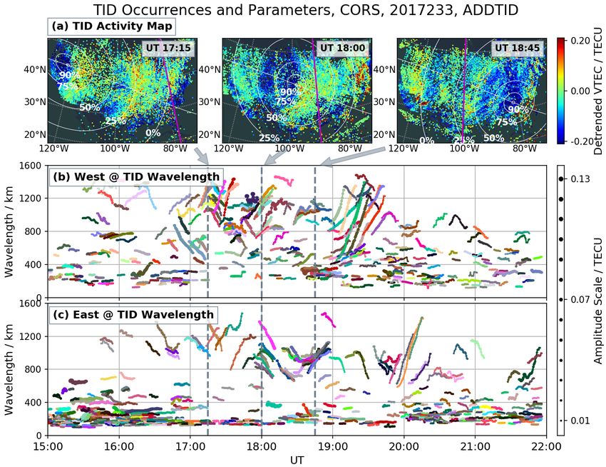
Remote Sens. 2018, 10, 1710                                                                          2 of 24

satellite system (GNSS) ionospheric sounding [3] among others. Salah et al. [1] and Le et al. [4] observe
the consistently remarkable depletion of the electron density in F region as a direct consequence of the
decreased ionizing radiation in the ionosphere. Chimonas and Hines [5] point out that gravity waves
generated in middle neutral atmosphere by the eclipse-induced radiative cooling, should build up a
bow wave propagating up to E-F region of ionosphere and forming TIDs when the moon’s shadow
sweeps at supersonic speed. Furthermore, Chimonas [6], Fritts and Luo [7] and Eckermann et al. [8]
model and analyze the occurrence, structure and characteristics of the bow wave of atmospheric
gravity waves. Davis and Da Rosa [9], Cheng et al. [10] and Zerefos et al. [11] observe the wavelike
ionospheric disturbances of atmospheric gravity waves at the D-F1 region during the solar occultation
by the moon, but show weak and ambiguous correlations with the bow wave characteristics due to the
difficult observation conditions and the existence of other factors that have a greater influence, such as
geomagnetic activity, regular solar terminator, etc. In particular, the large dense ground-based GNSS
observation network can be used as global ionospheric sensor network to detect and characterize the
time-varying and space-varying electron density fluctuations of the ionosphere. The GNSS observation
network in particular can be used to measure the disturbances in the ionosphere generated by the
transit of the moon’s shadow. Liu et al. [12] presented the observations of bow and stern waves in the
ionosphere induced by the solar eclipse of 22 July 2009, nevertheless the observations were to a certain
extend incomplete because the GNSS network only partially covered the affected region.
      In the case of the 2017 solar eclipse, which crossed the United States, the contribution of
this work is to provide a detailed characterization of the ionosphere’s response to the eclipse’s
transit. This is due to the fact that in the eclipse passed through an area densely covered by the
GNSS observation singular network in the United States. As previous works, we can mention
for example, Hernández-Pajares et al. [13] where the authors show the footprint of total electron
content (TEC) decrease in the global TEC map during the eclipse, and in Coster et al. [3] the
authors note a consistent and significant TEC depletion above US and also the presence of large scale
travelling ionospheric disturbances in detail during eclipse transit. In Zhang et al. [14] the authors
show three different patterns of eclipse-induced ionospheric perturbations and their approximate
characteristics such as the bow-shaped TEC depletion along the totality, the clear behavior of
ionospheric bow waves of atmospheric gravity waves and large scale ionospheric waves. In Nayak
and Yiğit [15] the authors show two kinds of travelling ionospheric disturbances of atmospheric
gravity waves in different intensities, the stronger ones occurring along the totality and the other
in the region with lower eclipse magnitude. Finally in Sun et al. [16] the authors describe the
occurrence and characteristics of the large scale V-shaped wavefront as a shock wave in F region
of the ionosphere. These observations done by means of a dense GNSS network are consistent with the
TEC variation prediction by Huba and Drob [17], the simulation of atmosphere-ionosphere response
(see McInerney et al. [18] and Wu et al. [19]) and the ionosphere observations by other techniques
such as Reinisch et al. [20] and Bullett and Mabie [21]. This indicates the ability of ground-based dense
GNSS networks to accurately detect eclipse-induced disturbances.
      In the above mentioned literature, most of the authors analyze the disturbances created by the eclipse
based on maps by means of visual inspection. In contrast, in this work we will use an algorithm that
automatically detects TIDs from a large number of measurements from a GNSS network. These measures
include observable fluctuations along the lines at all heights of the ionosphere. Also the bow-shaped
gravitational waves. In particular, in this work, we will compare each of the estimated disturbances
by means of the Atomic Decomposition Detector of Traveling Ionospheric Disturbances (ADDTID)
algorithm with a visual representations of the maps where the associated phenomenon is observed.
      In summary, the contribution of this work will be the temporal characterization of the ionospheric
disturbances associated with the eclipse of 21 August 2017, by means of an algorithm capable of
quickly detecting the temporal variation of the characteristics of multiple simultaneous TIDs. For this,
we have used the ADDTID algorithm (see details of the theoretical background and implementation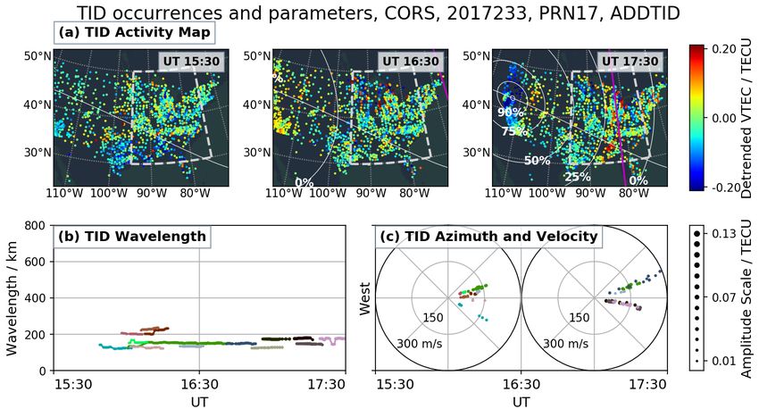
Remote Sens. 2018, 10, 1710                                                                               3 of 24

in Yang et al. [22]), which detects several simultaneous TIDs and yields the changes in wavelength,
azimuth and velocity of each wave as a time series.

2. Observation Data and Space Weather
     In order to describe the effects of the eclipse on the ionosphere above the United States, we used
data from GNSS receivers. The source of the GNSS data is provided by the Continuously Operating
Reference Stations (CORS) network of the National Geodetic Survey (NGS). This network consists
of almost 2000 ground-based continuous GNSS stations densely distributed in the United States [23]
(see Figure 1).

      Figure 1. GNSS receivers distribution of CORS in United States and the path of totality for the solar
      eclipse in August 2017. Magenta dots denote the location of the GNSS receivers, the black dashed
      line the path of totality, the blue rectangular frame the West sub-network of CORS and the red the
      East sub-network.

      During the duration of the eclipse, the geomagnetic activity was very weak (the planetary
3-hour-range indices kp ≤ 3, see US Department of Commerce, National Oceanic and Atmospheric
Administration (NOAA) [24]), and the auroral electrojet activity was moderate (the AE index ≤500 nT,
see World Data Center for Geomagnetism, Kyoto [25]). Also there were no significant disturbances
originated by natural hazard phenomena such as solar flares, significant earthquakes or tsunamis,
that is, no corresponding ionospheric disturbances in the CORS-observing region recorded in [26–28].

3. Methodology
     In the introduction, we presented a summary of the possible explanations of the different types of
disturbances produced by the eclipse transit over the continent. These include bow waves and other
related disturbances. These bow waves consist of several simultaneous TIDs induced by different
causes, among them, the upward atmospheric gravity waves [5]. In addition we detected early
perturbations, and perturbations that persist after the transit.
     In this study, the detection of several simultaneous TIDs was implemented in three steps: (a) The
GNSS data preprocessing, that obtains the ionospheric combination from the dual frequency carrier
phase data, and computes the detrended TEC data (Section 3.1); (b) the TIDs characterization by means
of the ADDTID algorithm that automatically detects them and estimates their parameters (Section 3.2);
(c) The details of subdivision criterion of the network for improving the performance of the ADDTID
algorithm (Section 3.3).
Remote Sens. 2018, 10, 1710 4 of 24
3.1. GNSS Preprocessing and Detrending
The preprocessing of GNSS data was done as follows: first we obtained the ionospheric
combination (also called geometry-free combination) L I (t) from the dual frequency carrier phases
L1 (t) and L2 (t), as the difference L I (t) = L1 (t) − L2 (t) (in length units). The L I (t) is an affine function
of the slant total electron content (STEC), which we will denote as S(t). This affine function consists
of a linear coefficient and an intercept, which takes into account the carrier phase ambiguity and
wind-up term. The main components of S(t) are the TEC trends such as diurnal variations and
elevation angle variation with low frequency and high energy, which we will denote as background
component. Besides, another component of S(t) of interest that has different frequency properties are
the ionospheric fluctuations, such as the TIDs.
A method for separating the TID component from the background component, consists of
computing the double difference (i.e., bandpass filter) of the time-series of measured L I (t). We will
denote this double difference as S̃(t) (see Hernández-Pajares et al. [29]). Taking into account the almost
constant intercept in L I (t) when no new losses of lock (cycle slips) occur, we group the time series
L I (t) into independent sub-series defined by the cycle-slips. In each sub-series, the intercepts can be
considered constant, and thus can be eliminated by the double time difference divided by −2, that is,
1
S̃(t) ≈ L I (t) − [ L I (t + ∆t) + L I (t − ∆t)] (1)
2
where ∆t is the detrending time interval, which determines the enhanced frequency bands of the TIDs
in S̃(t). Although there is no definite agreement about the characteristics of bow waves generated by the
eclipse (see the previous studies Chimonas and Hines [5], Zhang et al. [14] and Nayak and Yiğit [15]),
these studies suggest a periodicity of TIDs of 20–60 min. Therefore, we selected ∆t = 600 s for the
band pass filter in order to emphasize the eclipse-induced TIDs and also to greatly limit the effect
of typical medium scale TIDs with 10 min of periods (see Hernández-Pajares et al. [30]). This value
allows high sensibility to the TIDs with periods of 12–60 min. Attenuating the waves by a factor lower
than 1/2 the waves of periods less than 12 min or greater than 60 min, being relatively flat in this band.
The time evolution of the TIDs at different elevation angles is estimated from the detrended VTEC
Ṽ (t) which in turn is the projection of the detrended STEC S̃(t) by means of a mapping function
S̃(t)
M (t), i.e., Ṽ (t) = M(t) , see Hernández-Pajares et al. [31]. This method assumes that S̃(t) occurs
at the ionospheric pierce points (IPPs). These IPPs are located on a shell with the mean effective
height corresponding to the height where we assume that the TIDs commonly occur. We discarded
observations with an elevation angle of less than 15◦ as a compromise between obtaining enough TIDs
information and the effect of the angle on the mapping function errors.
We took 250 km as the mean effective height to detect these ionospheric disturbances. This is
justified by the following reasons: (a) Hernández-Pajares et al. [29] point out that the maximum MSTID
generation occurs at the height below hmF2 because the MSTIDs are generated by the interaction
between the neutral and ion particles. (b) In the case of this eclipse, Huba and Drob [17] predict the
electron density would decrease in E-F region between 150 and 350 km. (c) Nayak and Yiğit [15] and
Zhang et al. [14] point out that during the eclipse the height where the ionosphere shows the maximum
perturbation typically in the E-F1 region below hmF2, as the response to the atmospheric gravity
waves induced by the solar eclipse. (d) Zhang et al. [14] and Sun et al. [16] show the eclipse-induced
large scale TIDs should be generated at the F region. (e) The regular hourly height distribution of
peak electron density (hmF2) on this day ranged from 240 km to 310 km (obtained from National
Aeronautics and Space Administration/Goddard Space Flight Center (NASA/GSFC) [32], see the
International Reference Ionosphere 2012 model [33]).
In addition, the TID detection was performed independently for each GPS satellite, because
TID activity measured from the detrended VTEC maps could occur at different heights. In addition,
the analysis was performed taking this aspect into account.Remote Sens. 2018, 10, 1710 5 of 24
3.2. Summary of the Atomic Decomposition Detector of Traveling Ionospheric Disturbances Algorithm
The analysis of the data was done by means of the Atomic Decomposition Detector of Traveling
Ionospheric Disturbances algorithm (ADDTID, see details in Yang et al. [22]). This algorithm uses
data from a dense GNSS receiver network, and can detect and characterize TIDs from the ionospheric
piercing points (IPPs). The algorithm creates a dictionary of possible waves that encompass the
geographical area under study. The estimation is done using only the IPP samples, and solving a
convex optimization problem with a regularization term. This algorithm determines the TIDs as the
elements of the dictionary that best approximate the observations at the IPPs. Stating the problem in
this way has several advantages, mainly, that the number of possible waves to be detected does not
have to be stated beforehand. Also, and perhaps the most challenging aspect of the estimation problem,
the algorithm can work with non uniform spatial sampling, including the presence of directions with
higher density of sensors, or regions of the network lacking sensors.
In this article (following the presentation in Yang et al. [22]), we have used a dictionary of plane
waves. The model of the waves that gives rise to the elements of the dictionary have the following form,
A ( x, y, t) = A0 cos ~k · ( x, y) − ω (t − t0 ) + ϕ0 (2)
where ~k is the 2D angular wave number vector, with the module ~k = 2π
λ ; λ is the wavelength and
~k
the normal vector = (cos θ, sin θ ) points in the direction of propagation of the wave. The wave
|~k|
amplitude is A0 . The terms ω, t0 and ϕ0 are the angular frequency, the starting epoch and initial phase
of the TID wave, respectively. The corresponding ith dictionary element Ti ( x, y) at epoch t is defined
as follows:
2π
Ti ( x, y) = cos ( x cos θi + y sin θi ) + ϕi (3)
λi
The element Ti ( x, y) of the dictionary is characterized by: λi wavelength, ϕi phase, and θi wave
azimuth. The parameters of each element of the dictionary (θ, λ, and ϕ), are quantized as real numbers,
with values restricted to realistic ranges.
The dictionary D is constructed by the concatenation of the set of N elements Ti ( x, y), reshaped
as vectors, giving an array D, defined as D = [ T1 , T2 , T3 , ..., TN ]. The elements Ti ( x, y) are generated by
assigning to the parameters {λ, θ, ϕ}, all possible feasible values in a quantified range. Each element
Ti ( x, y) consists of a grid of Pv rows and Ph columns, i.e., a uniform sampling of the geographical
region of interest. Then, the array is reshaped to a vector Ti of dimension Pv × Ph . Please note that the
observations correspond to the IPPs; hence, in the estimation of the vector, αt will be done only with
the coordinates ( x, y) corresponding to measured IPPs. Therefore given a dictionary D, we estimate a
set of coefficients at time t, which we denote as αt , such that the observation V, is approximated by
the product V ≈ Dαt . The observation vector V, is defined by the values observed at the IPPs of each
satellite. In order not to change the notation, from now on the dictionary matrix D, is defined so that
for each element of the dictionary we only extract the components at the observed IPPs.
The parameter vector αt , is estimated by means of a trade-off between a loss function (i.e., how well
we approximate the observations by means of the model) and a regularization term (i.e., constraints on
the possible solutions). The regularization term is used in order to guarantee that the solution should
be sparse, that is, only a small set of elements of the dictionary will contribute to the approximation.
An estimation technique that allows for the trade-off with a sparse set of coefficients is the LASSO
(see for instance Hastie et al. [34]), where the norm on the loss function is `2 , and the norm on the
regularization term is `1 . Thus the optimization problem to be solved is,
1
α?t = arg min kV − Dαt k`2 + ρkαt k`1 (4)
αt 2Remote Sens. 2018, 10, 1710 6 of 24
The parameter ρ controls the level of sparsity of the solution, and is determined automatically
from the data, as explained at Yang et al. [22].
3.3. Justification of the Network Subdivision Criterion to Enhance the Performance of the ADDTID Algorithm
The model ADDTID, assumes that the TIDs propagate in the form of plane waves. In practice,
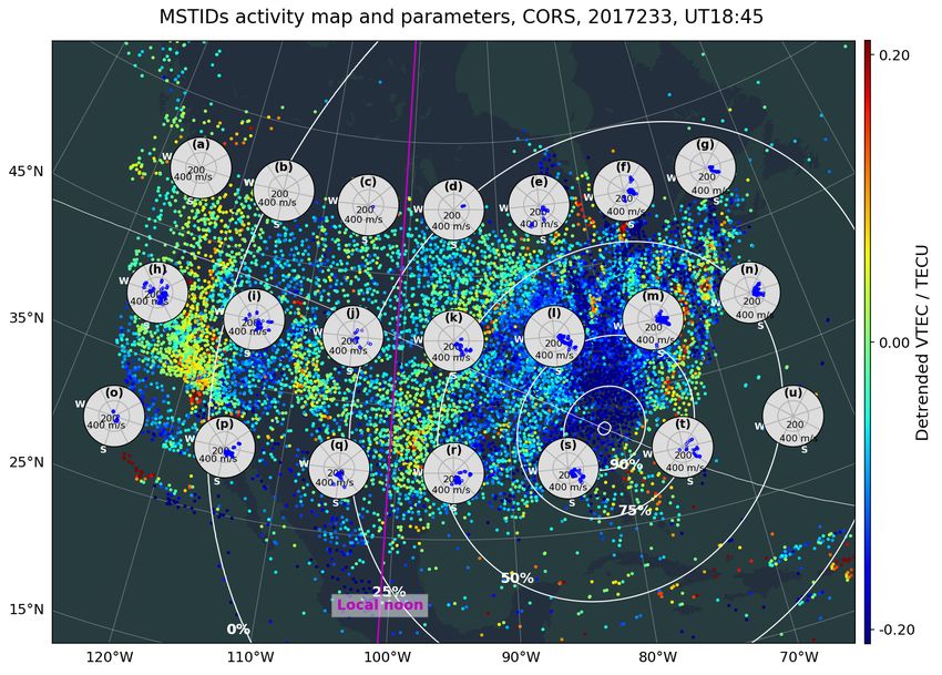
the TIDs, as is shown in the Figure 6a, show a propagation pattern that follow the shape of the eclipse
isopenumbra lines (shown in white). These isopenumbra lines for different elevations show a shape
similar to an ellipse. In this case the equivalent to the eccentricity of an ellipse, depends on the
inclination of the eclipse’s shadow. These ellipse-shaped shadow gradually decreases the amount
of solar irradiance incident on the atmosphere. For the physical intuition of the inclinations and
obscurations see Figure 2. This gradual obscuration in space and time, causes the electron density
oscillations, that follow a complex and complicated response at different scales. An example of the
wealth of phenomena is shown in Figure 6a, which shows the disturbances follow the isopenumbra
lines for different inclinations. The disturbances include: bow-shaped wavefronts, partial circular
wavefronts, receding ripples and planar wavefronts in different scales. As a precedent, in which similar
phenomena are observed see Zhang et al. [14] and Sun et al. [16]. This suggests that a natural model
for the dictionary matrix D of the ADDTID algorithm, should include all possible quadratic patterns
of wave propagation. Nevertheless this is prohibitive from the computational point of view because
the size of the dictionary grows by a polynomial of the number of parameters.
Figure 2. Variations of penumbra, umbra and solar irradiance at three moments of the eclipse,
blue solid-line circles denote the penumbra in 25%, 50%, 75%, 90% of obscurations and the umbra,
blue dashed line represents the eclipse totality, the color map shows the global horizontal irradiance at
the height of 250 km.
As mentioned in Section 3.2, the ADDTID algorithm can approximately estimate these circular
waves as compositions of local planar waves. This means, for instance, that a given wave front of a
bow wave, would be detected as two planar waves propagating in symmetric directions at each side of
the main direction of propagation. In Figure 5, we show a visual example of the validity of the plane
wave approximation. In this figure, the detrended VTEC maps over the local net of California show a
near plane wave structure, which corresponds to the detected waves at the scatter plot (Figure 5b,c).
This scatter plot at 17:15–17:45 UT, shows that the detected planar TIDs are distributed along two main
directions that are symmetric with the main propagation azimuth that is approximately 90 degrees.
At simple glance, we can see on the map measured at the same moment, there are two flat fronts, with
the same azimuths detected by the algorithm. (Note in the subplots at Figure 5e–h, the alignment of
dots of same intensity distributed following lines).
This indicates that the size of the measuring network has to be such that the curvature of the
wavefront should be small. As is shown in Figure 1, we divided the CORS GNSS network that covers
the US into several smaller subnetworks, each covering an area where the resulting TIDs can be locally
approximated by a planar wave. The partition into subnetworks was done taking into account the
different scale bow waves reported in Zhang et al. [14] and Sun et al. [16], the scheme of division isRemote Sens. 2018, 10, 1710 7 of 24
two sub-networks, the West Coast and the East Coast. This is because the ADDTID algorithm that was
used for detecting the TIDs assumes that the waves to be detected are planar and cover a significant
part of the stations. This hypothesis is approximately true if the whole net is partitioned into subnets.
A feature of the algorithm that is relevant for this study, is that the estimation is robust to non uniform
sampling and the geographical orientation of the set of stations.
In a more detailed way, the division of the network is justified because of the following reasons.
(a) The disturbances that are generated by the eclipse can be approximated locally as plane waves,
but at the scale of the whole network the curvature can be significant (see for instance Figure 6).
Thus, the size of the partition of the network was such that inside a partition the wave front can
be approximated as planar, and corresponding parts away from the umbra, which exhibit a greater
curvature, are included in the neighbouring partition. (b) As can be seen in Figure 1, the central part
of the network has a lower density of stations, which has an effect in the accuracy of the estimation.
Therefore it is a natural region for deciding the border between partitions. (c) We allowed for an
overlap of about 10% between subnetworks, in order to be able to check the consistency of the estimates
between them. (d) Finally, the partition is also justified because the disturbances caused by the eclipse
were different from one geographical area to another.
An additional benefit is the fact that the propagation of the waves at either coast follow similar
azimuths and wavelengths, but the velocities may sometimes have a different sign. As an example
of this see the TID maps in Figures 3d and 4d, where the wavefronts in the west and east parts
have differences in their azimuth and wavelength. Another benefit of the geographical partition into
sub-nets is that this allows for explaining phenomena that are qualitatively different and might appear
mixed if the analysis were done with the entire network.
TID occurrences and parameters, CORS, 2017233, PRN2
1500 1.0 (b) Velocity/Azimuth (c) Velocity/Azimuth
(a) Wavelength UT16:15-16:45 UT16:45-17:15 0.13
Amplitude Scale / TECU
0.8
1125
Wave length / km
0.6
750 W W 0.07
0.4 100 100
200 200
375 300 300
0.2 400 (m/s) 400 (m/s)
0.01
0 0.0
UT16:15 UT16:30 UT16:45 UT17:00 UT17:15
0.0 0.2 S 0.4 0.6 S 0.8 1.0
1.0
45°N (d) TIDs map @ UT16:50 (e) UT 16:55 (f) UT 17:00 0.20
0.8
Detrended VTEC / TECU
30°N
0.6 90%
75%
50% 0.00
(g) UT 17:05 (h) UT 17:10
0.4
15°N
25%
0%
0.2
0° Local noon
0.0 -0.20
0.0 135°W 0.2 120°W 0.4 105°W 0.690°W 75°W
0.8 1.0
Figure 3. Time-variation plots of the TIDs parameters, when the penumbra of about 50% magnitude
covers the west part of CORS GNSS network, estimated from satellite PRN2. (a): time evolution of the
TIDs wavelengths, (b,c): velocity vs. azimuth polar plots at intervals of half an hour, the continuity
and amplitude of TIDs are coded by colors and the dot sizes respectively. (d–h): TIDs activity maps at
16:50 UT, 16:55 UT, 17:00 UT, 17:05 UT and 17:10 UT, the white arcs marked with percentages are the
iso-penumbra lines on the IPPs at the altitude of 250 km. The diagonal white line is the trajectory of the
umbra’s center and the magenta line marks the local noon at the altitude of 250 km.Remote Sens. 2018, 10, 1710 8 of 24
For instance in Figure 6, we show a measurement done with all the satellites and stations.
From visual inspection, one can see that the wave forms follow the curvature of the umbra, and that
the wavelengths are not uniform. In addition, in the east section of network (about 100◦ W to 80◦ W of
longitude, and 28◦ N to 50◦ N of latitude) a set of ripple waves can be observed, that have a much lower
wavelengths compared with the main ones that cover the whole continent. This idea of partitioning
the network as a function of the scale of the disturbances allows for analyzing the ripples as medium
scale TIDs, by dividing CORS into subnetworks with the geographic scale of 10◦ × 10◦ (latitude vs.
longitude), see details in Section 4.5.
TID occurrences and parameters, CORS, 2017233, PRN12
1500 1.0 (b) Velocity/Azimuth (c) Velocity/Azimuth
(a) Wavelength UT18:45-19:15 UT19:15-19:45 0.13
Amplitude Scale / TECU
0.8
1125
Wave length / km
0.6
750 W W 0.07
0.4 100 100
200 200
375 300 300
0.2 400 (m/s) 400 (m/s)
0.01
0 0.0
UT18:45 UT19:00 UT19:15 UT19:30 UT19:45
0.0 0.2 S 0.4 0.6 S 0.8 1.0
1.0
45°N (d) TIDs map @ UT19:05 (e) UT 19:10 (f) UT 19:15 0.20
0.8
Detrended VTEC / TECU
30°N
0.6
0.00
(g) UT 19:20 (h) UT 19:25
0.4
15°N 90%
75%
0.2 50%
25%
0°
0%
0.0 Local noon -0.20
0.0 135°W 0.2 120°W 0.4 105°W 0.690°W 75°W
0.8 1.0
Figure 4. West coast sub network. (a–c): wavelength and velocity/azimuth plots. (d–h): lines of equal
penumbra TID parameters plots when the penumbra of about 0% magnitude in the west part of CORS
GNSS network, estimated from satellite PRN12 and TIDs activity maps at 19:05 UT, 19:10 UT, 19:15 UT,
19:20 UT and 19:25 UT. The plot is organized as in Figure 3.
4. Results and Discussion
In this section, we will analyze the diverse types of ionospheric disturbances generated during
the eclipse transit at a height of 250 km. The analysis will be done both, by means of the ADDTID
algorithm and by visual inspection of the maps. The TIDs that we detected (and visually verifed)
show a wide range of features that depend on the elevation angle change, the footprint, size, azimuth
and velocity of the umbra. We have structured the analysis of the generated TIDs, first following the
temporal evolution of the eclipse and finally a global summary:
1. Time-varying TIDs analysis of the early and final moments of the eclipse observed from California
in Section 4.1.
2. Simultaneous TIDs with multi-scale wavelengths presented during the middle stage of the eclipse
observed from California in Section 4.2.
3. In Section 4.3, we summarize the detected multi-scale TIDs during the whole transit of the eclipse.
4. In Section 4.4, we show in detail the features of bow wave consisting of large scale TIDs, and in
particular the estimated opening angles.
5. The medium scale TIDs in the penumbra are described in Section 4.5, such as partial circular
waves, apparition of receding ripples among others.
6. In Section 4.6, a set of early MSTIDs at the east coast is detected before the arrival of penumbra.Remote Sens. 2018, 10, 1710 9 of 24
4.1. Time Varying TIDs Wavelengths in the Early and Final Stages of Eclipse Transit
In this section, we will describe the temporal evolution of the TIDs in the early and final stages of
the eclipse. The description will be carried out simultaneously, by means of the parameters detected
with the ADDTID algorithm and by visual observation of the maps for verification purposes.
The disturbances that appear in the early and final stages of the eclipse, coincide with the
distribution of the TIDs when the umbra either is about to enter the continent or to leave it.
The eclipse-induced ionospheric perturbations would primarily be the consequences of the atmospheric
cooling effect at all heights. However, the response of the ionosphere to the cooling due to the rapid
variation of the penumbra is not well understood. As is shown in the model of Figure 2, where
the lines of iso-penumbra and umbra (see computation details in Montenbruck and Pfleger [35]),
are superimposed with the simulated global horizontal irradiance color map (see simulation details in
Andrews et al. [36]). The consequence is that the movement of the shadow, generates fast space-varying
and time-varying cooling effects at the atmosphere. This movement is in part, due to change in the
grazing angle at the different stages of eclipse. The main feature is that for grazing angles of the umbra,
the penumbra creates elliptic-like shadows of gradual obscuration. On the other hand, for vertical
angles the shadows of the penumbra show less eccentricity. The geometry of the problem gives rise to
a changing velocity of the penumbra shadows. That is, while the angle increases steadily, the velocity
of change of the elliptical shadow of the penumbra will be high during the transition from grazing
angles to medium angles.
As reported in Zhang et al. [14] and Sun et al. [16], the eclipse-induced ionospheric disturbances
can be classified into two categories with distinct scales: (a) bow-shaped large scale TIDs and
(b) medium scale TIDs of bow waves, originated respectively by in situ and not in situ gravity
wave effects. In this subsection we will study both kinds of the disturbances in a separate subnetwork
centered at California, (see in Figure 1). The California network is defined as a more restricted
geographical area, which covers a smaller region, with a high density of stations allowing a more
clear detection and modeling of the TIDs, because they can be locally approximated by a planar wave.
Another reason we limit ourselves to this subnet is that for grazing angles, the distribution of TIDs will
be very different across the continent, which could result in a mixture of different effects. The result of
this change in angle, is the emergence of a set of TIDs, with a wavelength time evolution that follows a
parabolic shape. This parabolic shape of the evolution in time of the wavelength is common to the
entering and departing phases of the umbra and penumbra.
4.1.1. The Early Stages of Eclipse Transit
Figure 3 (GNSS observation of GPS satellite PRN2), shows the entry phase of the eclipse.
Figure 3d–h show TEC maps of the west coast between 16:50 UT and 17:10 UT. Superimposed over
these maps, we show the isopenumbra lines from 90% to 0% of obscuration, when the umbra is over
the Pacific ocean. By means of the algorithm presented in Montenbruck and Pfleger [35], the lines of
isopenumbra are depicted at an altitude of 250 km, and the measurements over the set of stations over
the continent. The lower right part, shows a zoom of the TEC evolution at time intervals of 5 min.
The upper part of the figure shows the time evolution of the TID wavelengths (Figure 3a) and the two
polar plots of azimuth vs velocity (Figure 3b,c). Wavelengths, azimuth, velocity and amplitude are all
estimated by the ADDTID algorithm. Please note that the azimuths and wavelengths given by the
ADDTID coincide with the values that can be estimated at glance from Figure 3d–h. In addition we
have overlaid on the maps, the projection of the detected points to a straight line with an inclination
equal to the most common azimuth of the detected TIDs. Please note that the projection allows the
visual inspection to determine the approximate wavelength of the disturbances and the propagation
azimuth. As a supplement to Figure 3, we have posted on the Internet VTEC variation films during
the eclipse in [37].
Next, we will describe the evolution of the TID estimated by means of the ADDTID algorithm
and we will contrast it with the measured maps. Beginning at 15:55 UT, the penumbra contactsRemote Sens. 2018, 10, 1710 10 of 24
the ionosphere over west US region, and from then on, increasingly covers this region. The time
evolution of the TIDs in the early 30 min, show Medium Scale TIDs (MSTIDs) with a wavelength in the
range of 250 to 300 km, a propagation following an azimuth towards the southeast. Please note that
although the distribution of velocities is broad, most of the observations (75%) are concentrated in the
range 150–300 m/s. The amplitudes during this time interval decreased from 0.08 to 0.02 TECU.
The color-coding convention we have followed assigns a different color to each continuously
detected TID sequence. The same colors have been assigned to the wavelength paths and points
in the azimuth vs. velocity diagram. The MSTIDs detected during local morning hours show
the typical daytime pattern in summer, mostly driven by solar terminator, see similar reports in
Hernández-Pajares et al. [30]. At about 16:45 UT, the MSTIDs suddenly disappear, and a set of long
wavelength TIDs emerge, that show a downward trend starting at a value of 1125 km. This change
coincides with the arrival of the penumbra at a level of obscuration of 50–75%, as can be seen from the
geographical distribution of the iso-penumbra lines at Figure 3d. The azimuth of the long wavelength
TIDs moves 10 degrees to the east, and the velocity as seen in Figure 3c decreases to 150–50 m/s and
the period decreases to a range of 3–0.75 h. This can be confirmed by visual inspection of Figure 3d–h.
Meanwhile, the umbra above the Pacific ocean moves toward to east at speed of about 3000 m/s.
Around 17:15 UT, 55 min after the onset of the penumbra reaches the network, the penumbra reaches
a 50% obscuration, and the wavelength of the TIDs converges to a value of 400 km. As shown in
Figure 5, this occurs a few minutes after the umbra contacts the California network.
The phenomena that we have described can be explained from the physical point of view in
several ways (see discussion of the literature on this topic in the introduction). Zhang et al. [14]
observed the penumbra-induced TIDs and recognized as the partial bow waves which should
originate from the neutral atmosphere when the ground shadow is of about 50% magnitude. The
time interval between the onset of TIDs and the time when the penumbra first arrives in California
is compatible with the 0.5–1 h delay range of the onset of TIDs according to Liu et al. [12] and
Nayak and Yiğit [15]. Another phenomena, that are observed in this paper are the bow waves
and related disturbances, and the different delays in the apparition of the ionospheric disturbances.
Shock waves are believed to originate from gravity waves in the middle atmosphere, due to the
umbra moving at supersonic speeds. On the other hand, the penumbra that partially covers the solar
radiation produces a cooling mechanism different from the umbra. This effect encompasses several
frequency bands, Huba and Drob [17] indicate that the moon blocks the irradiance of ultraviolet light
(uniform in the solar disk) in a similar way to light in the visual spectrum. In Kazadzis et al. [38], it is
observed that a significant part of the ozone column decreases when the obscuration associated with
darkness exceeds 70%. As the column variation in the ozone layer, absorbs most part of UV radiation,
the cooling effects by the low obscuration penumbra were not enough to break the heat balance in
the middle atmosphere. Therefore, these TIDs observed tens of minutes prior to the coverage by the
50% obscuration penumbra, might have a different origin. The global horizontal irradiance of the
region covered by the umbra and penumbra is depicted in the diagram of Figure 2. The decreasing
intensity of the irradiance from center outwards, generates different cooling effects, similar to a solar
terminator, with a very fast diurnal variation. For instance, Huba and Drob [17] report the delayed
variation of irradiance of X-ray and Extreme UV (EUV) because 10–20% contribution in these bands
are generated at the solar corona, which is not covered by the moon. While the X-rays and EUV
photons which are the primarily source of photoionization in the ionosphere, is occluded by the
moon. On the other hand, Coster et al. [3] observed the TEC depletion follow with a short time delay
the radiation distribution induced by the umbra and to the percentage of penumbra, and reported
the penumbra-induced large scale TIDs activities could be originated in situ with the thermosphere.
This explains the above mentioned set of long wavelength TIDs, that appeared suddenly when the
coverage of the penumbra reached the 50% of obscuration, and the following convergence of the TIDs
about a few minutes after the umbra reaches the network. Also is compatible with the ionosphericRemote Sens. 2018, 10, 1710 11 of 24
disturbances reported by Le et al. [4], Müller-Wodarg et al. [39] and Sun et al. [16], which would be
directly generated in thermosphere.
Figure 3 shows that the wavelength trajectory of long wavelength TIDs follows a descending
parallel parabolic shape. This path is compatible with decreasing the distance between the isopenumbra
lines. That is to say, the solar irradiance gradient increases as the angle of the shadow increases from
6 degrees to 40 degrees, with the consequent reduction in the rate of variation of the isopenumbra
lines. At the same time, the direction of propagation (southeastbound) of TIDs is perpendicular
to the isopenumbra lines over the California network. The cooling effect on the California area
increases considerably as the angle and speed increases. This speed is supersonic at the heights where
disturbances occur. In conclusion, this shows that the deceleration of the rate of change of the area of
the penumbra and the decrease of the such area, is associated with a decrease of the wavelength of the
TIDs. This happens in spite of the fact that the speed of the TIDs is slower than that of the umbra.
As for bow waves, the shape of the TIDs induced by the penumbra is consistent with bow waves
of variable aperture in the south direction. One aspect to note is that the geomagnetic lines give rise to
a slight deviation towards the equator due to the low geomagnetic activity, as mentioned in Section 2,
see Coster et al. [3].
4.1.2. The Final Stages of Eclipse Transit
In Figure 4 we show, for the departing phase of the eclipse. For more details see the movie in [40].
The measurement has been made in the California subnet when the umbra is over the Atlantic Ocean,
which results in a grazing angle of the penumbra. The parameters shown in the figure were estimated
on the west part of CORS GNSS network, using the GPS satellite PRN12. The temporal evolution of
the wavelength shows, for the departing phase, a complementary behaviour to that observed in the
entering phase of the eclipse. The differences are due to the fact that the decrease rate of change of the
elevation angle of the moon is not exactly the opposite of the entering phase of the eclipse (see Figure 2).
On the other hand, the azimuth of the detected wavefronts is compatible with the direction of the
isopenumbra lines over the network.
At about 19:35 UT the TIDs with increasing wavelength get weaker and finally disappear when
the wavelength is over 1200 km. Subsequently, the activity of the disturbances decreases significantly,
after which only very low intensity TIDs are detected. These disturbances have an azimuth opposite
to that of the typical disturbances of this time of year.
The TIDs that have been detected show similarities with those of the initial stage, in the sense that
the direction of propagation is perpendicular to the isopenumbra lines, the range of velocities is similar,
and they are not significantly affected by the geomagnetic fields. A difference with respect to the TIDs
of the initial stage of the eclipse is that the propagation is in the opposite direction to the movement
of the shadow, which indicates that there may be no relation with the variation of the penumbra.
In addition, these TIDs occur at the time when the shade is at its lowest, i.e., when the shadow leaves
the California region, about 105 min after the umbra and about 85 min after the isopenumbra level
of 50% leaves the subnetwork. This suggests that the fluctuations of the ionosphere are not due to
the direct cooling effect in the thermosphere, but are upward gravity wave disturbances originating
in the neutral atmosphere. Nevertheless the behavior of the TIDs differs from Coster et al. [3] and
Zhang et al. [14], Chimonas and Hines [5] explains the above-mentioned behavior of disturbances
by stating that long period atmospheric gravity waves cannot ascend from the point of generation
at a sufficiently steep angle. From theoretical considerations, they conclude that the period of the
disturbances is 3 to 4 h, which is in line with the results of the estimate we have made. The period of
the TIDs detected in F region, increases gradually from 1 to 5 h. Similarly, in a study related to the 7
March 1970 eclipse, Davis and Da Rosa [9], in synchrony when the penumbra boundary (i.e., 0% area)
left the network, observed westward TIDs in the form of decreasing amplitude shock waves with
gradually increasing periods. However, the period of the TIDs estimated was of about 25 min, which
was not consistent with the predicted long period in Chimonas and Hines [5].Remote Sens. 2018, 10, 1710 12 of 24
4.2. General Description of the Multi-Scale TIDs (Medium and Large) in the Middle Stage of Eclipse Transit
In this subsection, we show the presence of the multi-scale TIDs, i.e., medium and large, measured
from the California subnetwork.
Figure 5 shows the characteristics of ionospheric perturbations when the umbra crosses the
California subnetwork. For more details see the movie in [37]. The umbra contacts the atmosphere
above this region at a height of 250 km at about 17:11 UT and leaves the subnetwork at about 17:42 UT.
As mentioned in Section 4.1 during the early stage, the set of parallel wavelength-varying TIDs from
17:00 UT follow a downwards trajectory, converging towards a medium scale wavelength TID of
about 400 km, 4 min after the arrival of the umbra. Almost simultaneously, with a slight delay due
to the response of the ionosphere (see Figure 5a), a disturbance suddenly appears with a wavelength
of 1125 km at about 45 degrees of azimuth, nearly 90 degree to the north of the medium scale TID
azimuth. This perturbation corresponds to the three segments of the trajectory observed at Figure 5a.
Please note that the trajectories of large-scale disturbances are reflected on the projection (in red) in
Figure 5e–h, as almost two cycles of a sine wave with a wavelength compatible with 1200 km.
TID occurrences and parameters, CORS, 2017233, PRN2
1500 1.0 (b) Velocity/Azimuth (c) Velocity/Azimuth
(a) Wavelength UT17:00-17:30 UT17:30-18:00 0.13
Amplitude Scale / TECU
0.8
1125
Wave length / km
0.6
750 W W 0.07
0.4 100 100
200 200
375 300 300
0.2 400 (m/s) 400 (m/s)
0.01
0 0.0
UT17:00 UT17:15 UT17:30 UT17:45 UT18:00
0.0 0.2 S 0.4 0.6 S 0.8 1.0
1.0
45°N (d) TIDs map @ UT17:26 (e) UT 17:28 (f) UT 17:30 0.20
0.8 25%
50%
Detrended VTEC / TECU
30°N 75%
0.6
90%
0.00
(g) UT 17:32 (h) UT 17:34
0.4
15°N
0.2
0° 0%
Local noon -0.20
0.0 135°W 0.2 120°W 0.4 105°W
0.0 0.690°W 75°W
0.8 1.0
Figure 5. Time-variation plots of the TIDs parameters, when the umbra covers the west part of CORS
GNSS network, estimated from satellite PRN2, organized as Figure 3. TIDs activity maps shown at
17:26 UT, 17:28 UT, 17:30 UT, 17:32 UT and 17:34 UT.
Both disturbances persist between 17:15 UT and 17:45 UT, the long scale disturbance with an
amplitude of about 0.11 TECU and the medium scale of about 0.05 TECU for other. The spread in
terms of azimuth of both perturbations shifts several degrees towards the east, which is compatible
with the lines of equal penumbra and perturbations shown in Figure 3. The disturbance of longer
wavelength can be found by visual inspection in Figure 5.
Although the observed velocities of both sets of TIDs are lower than the typical velocities for large
and medium scale TIDs, there is a consistency, in the sense that the large scale TIDs propagate at a
double speed compared to the medium scale waves.
Note also, that of the size and distribution of the stations is lower than the area covered by the
bow wave, therefore only one of the branches of the bow wave is detected in the figure. Another effect
that can be observed at the maps and the wavelength vs. time figure (Figure 5), is that the amplitudeRemote Sens. 2018, 10, 1710 13 of 24
of the large scale TIDs is greater than in the case of the medium scale TIDs (note that the amplitude
is coded by the size of the dots). An additional observation from this Figure, is that the azimuth of
the TIDs does not coincide with the trajectory of the eclipse on the maps. This might be related to
the movement of the bow wave fronts both in large and medium scales. In the figure there are also
disturbances that appear in advance of the umbra.
These medium scale TIDs are a response of the ionosphere to the transition from the penumbra
to the umbra, which generates the ionospheric wave in situ. Whereas long scale TIDs are also due
to the effect of the umbra on the ionosphere, with delay appearing after the umbra has already
moved away [16]. These TIDs originate in part due to the cooling effect of the umbra’s shadow,
creating gravity waves in the thermosphere.
4.3. Description of Ionospheric Disturbances during the Eclipse
In this section will characterize and describe the ionospheric disturbances related to the bow
waves during the transit of the eclipse.
By visual inspection, in the maps plotted at Figure 6a, one can see a bow wave that varies gradually
at the different stages of the eclipse (see more details in [41]). In the three maps, in addition to the
bow wave, it is also possible to observe disturbances in advance of the umbra, and in the wake of the
umbra (see similar observations in Zhang et al. [14]). The shape of the waveforms of the disturbances
are akin to the lines of iso-penumbra in Figure 2. That is, the disturbances in advance of the umbra
follow the shape of the lines of iso-penumbra. The disturbances in the wake of the umbra show an
elliptical curvature following the shape of the lines of iso-penumbra, and also ripples (Figure 6a at
18:45 UT) of lower wavelength with a complementary curvature.
Figure 6. (a): TIDs activity maps at 17:15 UT, 18:00 UT and 18:45 UT, similar display scheme with
the TIDs map in Figure 3. (b,c): Wavelength time evolution for the west subnetwork (b) and east
subnetwork (c), point color and size code organized as Figure 3. The grey arrows pointing to dashed
vertical grey lines indicate observation time.Remote Sens. 2018, 10, 1710 14 of 24
In Sections 4.1 and 4.2, we show on the west coast, the occurrence of disturbances at medium and
large scales, ranging from a few hundred to more than a thousand kilometers. This phenomenon can
be seen on the maps in Figure 6a. In Figure 6c, we also show that the measurements done on the east
coast, follow with a delay, the shape of the wavelength evolution on the west coast.
These ionospheric disturbances during the eclipse appear as patches of 2D non-concentric near
circular wave patterns, moving horizontally. Since the curvature of the TIDs over the region of each
network is small enough, the ADDTID algorithm will be able to correctly detect the disturbances and
estimate their characteristics. To better understand the spatial-temporal characteristics of large-scale
ionospheric disturbances and their relationship to the eclipse, the estimation has been made with the
entire CORS network. That is, the GNSS data used in the ADDTID algorithm correspond to the two
subnetworks into which we have divided the CORS network (see Section 2). Please note that each
subnet is at least twice the maximum wavelength. Figure 6b,c, show the time evolutions of the TID
wavelengths respectively detected from west and east subnetworks of the CORS network.
The disturbance in advance of the umbra that can be understood as an early bow wave. The origin
is due to the changes in temperature generated by the increasing penumbra, giving rise to disturbances
of lower intensity in comparison with the one that was generated by the umbra [4,39]. As the penumbra
moves at a higher speed for grazing angles, the perturbation due to the eclipse appears some time
before the umbra reaches the region covered by the stations. Also, follow a distribution similar to
concentric ellipses, which is due the change on the angle of the umbra over a sphere (see for instance
the diagram in Figure 2 and the previous discussion in Section 4.1). These disturbances in advance to
the bow wave can be observed clearly in Figure 6a at 17:15 UT.
The measures done at the stations over the west subnetwork show that the typical pattern of
MSTID at this time of the year, disappear completely, while on the east subnetwork, which is at the
other side of the continent, they are reduced in number. In both cases the behaviour of the large scale
TID (LSTID) change, in case of the west subnetwork there is a noticeably decrease in the wavelengths
of these disturbances. With a delay of about half an hour, the same phenomenon appears on the east
subnetwork. A remarkable aspect is the continuity between the MSTIDs and the LSTIDs, which can
be seen in Figure 6a or zoomed at Figure 3. Also it can be seen in Figure 7c,d from the azimuth
vs. velocity plot that the direction of the large scale disturbances in consistent with the direction of
propagation of the umbra. This continuity of the transition between MSTIDs and the LSTIDs and
vice versa can be observed at both networks. As for the LSTIDs propagation (Figure 6a at 17:15 UT),
the disturbances follow the lines of iso-penumbra and propagate in the direction of the movement of
the eclipse, except at the east edge of the continent, where the angle varies slightly, perhaps due to
propagation delay. Around 18:00 LSTIDs with similar behavior appear, with a greater opening angle,
and a direction that follows the movement of the umbra, see the more details in Section 4.4.
The complementary behaviour is shown in Figure 6a at 18:45 UT, where we observe the
disturbances that appear when the umbra is over the west coast. In this case we observe LSTIDs to the
west of the umbra that follow the shape of the lines of iso-penumbra, with wavelengths that increase
slowly from 700 km to 1300 km. In addition, at the same time, MSTIDs of lesser wavelengths, with a
front waves with a curvature of opposite sign. These MSTIDs have a wavelength of about 200 km,
and on the map appear as ripples that can be observed at the west of the umbra. This transition can be
seen more clearly in the zoom at Figure 4a, and the azimuth vs. velocity plot of Figure 4b,c, shows that
the perturbations propagate in opposite direction to the propagation of the umbra. In Section 4.5 the
MSTIDs which correspond to the ripples are explained in detail.
4.4. Description of the Large Scale Ionospheric Perturbations Related to Variable Angle Bow Waves
In this section we extend the characterization done in Section 4.3 of the behaviour of the large
scale ionospheric disturbances (i.e., LSTIDs) during the eclipse transit. The behaviour of the LSTIDs
during the eclipse is summarized in Figure 7, in which we show time-aligned: (a) wavelength pathRemote Sens. 2018, 10, 1710 15 of 24
(Figure 7a,b) and (b) velocity vs. azimuth polar plots (Figure 7c,d). This diagram will allow us to
understand the relationships between these characteristics throughout the eclipse transit.
1600
TID occurrences and parameters, CORS, 2017233, ADDTID
(a) West @ TID Wavelength
Wavelength / km
0.13
1200
800
400
1600
(b) East @ TID Wavelength
Wavelength / km
Amplitude Scale / TECU
1200
800 0.07
400
(c) West @ TID Azimuth and Velocity
West
500 500 500 500 500 500 500
1000 m/s 1000 m/s 1000 m/s 1000 m/s 1000 m/s 1000 m/s 1000 m/s
(d) East @ TID Azimuth and Velocity
West
500 500 500 500 500 500 500
1000 m/s 1000 m/s 1000 m/s 1000 m/s 1000 m/s 1000 m/s 1000 m/s 0.01
15:00 16:00 17:00 18:00 19:00 20:00 21:00 22:00
UT
Figure 7. Behavior of the LSTIDs during the transit of the eclipse (Time aligned). (a,b): time evolution
of the wavelength of the LSTIDs, (c,d): Azimuth vs. velocity polar plots at intervals of one hour,
red stars for the azimuth vs. velocity of umbra. The dot color and size (right bar) coding follows the
convention in Figure 3.
The LSTIDs shown at Figure 7a,b have similar wavelengths and velocities as the typical large
scale TIDs [42], nevertheless the directions as shown at Figure 7c,d are different, following the azimuth
of the umbra center, which is denoted in the polar plots with the red stars.
Before the arrival of the eclipse to the continent, the LSTIDs exhibited a quiet behaviour,
characterized by low amplitude and propagation mainly in the equator-east direction. The duration of
the disturbances was less than 15 min, the speed was low of about 100–200 m/s and with long periods
in the order of 1.5–2 h. At about 15:56 UT, the penumbra arrives first at the ionosphere 250 km above
the west coast of US, from then on, the penumbra increasingly covers this region. At the same time the
number of LSTIDs increases. During the time interval 16:10–17:15 UT, when the 10% iso-penumbra line
reaches the western US, the properties of the TIDs change. The LSTIDs now head eastwards, with a
marked increase in the speed (over 500 m/s). The wavelengths of the LSTIDs, decrease from about
1500 km to 800 km, and then increase above 1200 km. Please note that the delay between the west and
east US, in terms of the evolution of LSTIDs, is approximately half an hour, which is consistent with
the delay due to shadow propagation. This delay was computed from the shape of the wavelength
trajectory observed in the figure, in particular from the position of the minimum of the parabola that is
repeated at each coast.
At about 17:15 UT, a large number of LSTIDs suddenly appear, a couple of minutes after the umbra
arrives the west US. At the west network between 17:15 UT and 18:05 UT (about 18:05 UT, the umbra
leaves to the west part of US), the wavelength path of the LSTIDs shows a parabolic shape, the edges
of this trajectory are determined by the entering and leaving phase of the penumbra (see commentsRemote Sens. 2018, 10, 1710 16 of 24
in Section 4.1). The disturbances show an eastward propagation, with an azimuth scattering of 60
degrees and a speed range between 300 and 700 m/s.
In the velocity-azimuth diagram, the points associated with the bow wave are distributed in a fan
shape, which corresponds to an opening angle of the bow of 120 degrees, and a propagation with an
azimuth of 10 degrees. This fan also indicates the speed of each of the branches of the bow. The bow
wave follows the path of the umbra, which at this moment has an azimuth of roughly 10 degrees south
east and a velocity in the range of 1500–670 m/s in Figure 7c.
After leaving the western network, the activity of the LSTIDs gradually weakens until they
disappear. A similar behaviour with a time delay, is visible in the eastern network. However, there are
differences in the distribution and properties of LSTIDs on the east coast compared to those on the west
coast. When the umbra covers part of the eastern subnetwork between the 18:05–18:50 UT, the angle of
opening of the bow wave increases to about 135 degrees, while the umbra speed decreases to 650 m/s.
At this time, the bow wave in the eastern subnetwork shows a global deviation of 30 degrees south,
which is compatible with the azimuth changes of the umbra movement. Please note that the direction
of propagation of the bow wave, along with the two branches of the bow, follows the movement of the
umbra, with an deviation in azimuth. This deviation is about 10 degrees north east at 17:00–18:00 UT,
and about 5 degrees south east at 19:00–20:00 UT. The low activity of the geomagnetic field has little
influence on the movement of the ions, so the deviation may be due to the variation in the eccentricity
of the ellipses resulting from the penumbra, and to the rotation of the ellipse axes. The deviation and
lines of equal obscuration can also be seen on the TID activity maps.
In Figure 8, we show the relationship between the opening angle of bow wave with the velocity
of the umbra. The figure shows in green the measurement made by visual inspection on the maps
and in grey the estimation using the ADDTID algorithm, and also in blue a nonlinear fit of the
ADDTID opening angle to smooth the estimation errors. The manual measurement on the maps was
performed prior to the measurement obtained from the ADDTID algorithm. This confirms that the
ADDTID algorithm can detect wavefronts and matches the approximate measurements manually
estimated. The order of the measurements is methodologically correct, as it avoids biases due to
having observed first the measurement from the algorithm. This order is justified, was because once
the manual measurement was performed, a posteriori check by means of the ADDTID was made to
confirm whether the manual measurement was correct. The velocity of the umbra is computed by the
algorithm Montenbruck and Pfleger [35], and the time evolution follows a concave up parabolic shape.
During the transit over the CORS network, the part corresponding to the highest acceleration of the
umbra was located outside the network. Please note that, as the velocity slows, the degree of opening
of the bow wave increases for both two measurements. The moment when the umbra velocity reaches
a minimum is about 18:29 UT (see the mark in Figure 8), which coincides with the moment when the
iso-penumbra line of 0% is completely within the territory of the United States. The decrease in the
opening angle of the bow wave observed with about 3–5 min delay, is due to the increase in the speed
of the umbra. The estimated opening angle shows a higher noise from 19:00 UT on, when the umbra
has already left the continent and is now on the Atlantic Ocean, and thus the two arms of bow waves of
LSTIDs are not completely observed by CORS network any more, as shown in Figure 4. Therefore the
measurement by means of visual inspection is reliable only until 18:30 UT. The LSTIDs corresponding
to the measurements in Figure 8 show the small delay with respect to the umbra, and propagate at
a speed greater than the speed of sound in the middle atmosphere. Both these two characteristics
are consistent with the findings in Coster et al. [3] and Zhang et al. [14]. This behaviour does not
correspond to the gravity waves induced by the eclipse in the middle atmosphere [5], but to the shock
waves generated in the thermosphere, with a speed compatible with the acoustic velocity [16].You can also read