Detection of structures in the horizontal wind field over complex terrain using coplanar Doppler lidar scans
←
→
Page content transcription
If your browser does not render page correctly, please read the page content below
B      Meteorol. Z. (Contrib. Atm. Sci.), Vol. 29, No. 6, 467–481 (published online July 21, 2020)
       © 2020 The authors
                                                                                                            Measurement Techniques

Detection of structures in the horizontal wind field over
complex terrain using coplanar Doppler lidar scans
Bianca Adler1,2,3∗ , Norbert Kalthoff1 and Olga Kiseleva1
1
  Institute of Meteorology and Climate Research, Karlsruhe Institute of Technology, Karlsruhe, Germany
2
  Current affiliation: CIRES, University of Colorado, Boulder, CO, USA
3
  Current affiliation: NOAA Physical Sciences Laboratory, Boulder, CO, USA
(Manuscript received February 24, 2020; in revised form May 18, 2020; accepted June 15, 2020)

             Abstract
             Coplanar scans from three Doppler lidars are used to retrieve the horizontal wind field in a horizontal plane
             of about 5 km × 5 km in size above the city of Stuttgart in south-western Germany. Stuttgart is located in
             moderate mountainous terrain that is characterized by a basin-shaped valley (Stuttgart basin) which opens
             into the larger Neckar Valley. Using the retrieved horizontal wind field, which is available on 22 days with a
             temporal resolution of 1 min and a horizontal resolution of 100 m, we investigate the mesoscale structure of
             the horizontal flow in the valleys with respect to time of the day, stratification and wind above the mean ridge
             height, and determine how fast the cells in the convective boundary layer move downstream, i.e. we estimate
             the convection velocity. The measurements reveal a large spatial and temporal variability of the flow. During
             stable conditions, the flow below the mean ridge height is decoupled from the flow aloft and downvalley wind
             dominates in the valleys. At the opening of the Stuttgart basin into the Neckar Valley outflow dominates during
             nighttime, whereas inflow into the basin prevails in the early morning. During thermally unstable conditions
             the flow in the valleys is mainly coupled to the flow aloft with a preference for upvalley wind direction.
             Convective cells moving downstream are detected in the horizontal wind field and a method to estimate the
             convection velocity from the horizontal wind field measurements is presented. The mean convection velocity
             is found to be higher by 24 % than the mean horizontal wind speed at the same height and about similar to
             the wind speed 100 m further up.
             Keywords: urban atmospheric boundary layer, convection velocity, mountainous terrain, thermally driven
             circulation, convective cells, Urban Climate Under Change [UC]2

1 Introduction                                                                Kalthoff and Vogel, 1992; Kalthoff et al., 1998;
                                                                              Kossmann et al., 1998). The large spatial variability of
The atmospheric boundary layer (ABL) over complex                             the flow induced by the orography and the built-up areas
terrain is highly variable in space and time. This is                         imposes high demands on the observation strategy as ob-
due to the superposition and interaction of processes                         servation with a high spatial and temporal resolution are
on multiple scales. Convection, shear-driven turbulence                       necessary to capture the variability and characteristics of
and mesoscale thermally driven circulations (e.g. Adler                       the flow (e.g. Barlow, 2014). Point measurements on
and Kalthoff, 2014; Serafin et al., 2018) as well as                          towers are not only of limited representativeness, they
dynamically driven flows which form when air flows                            are also difficult to install in built-up areas and capture
over orography (e.g. Jackson et al., 2013; Adler and                          only the lowest part of the ABL.
Kalthoff, 2016) interact with each other and impact                               To investigate the spatial characteristics of the con-
the conditions in the ABL. The flow structure in the                          vective ABL, such as the size of the turbulent cells, the
ABL is crucial for the exchange of air masses in val-                         standard set-up involves in situ measurements on tow-
leys and basins with the layers aloft, i.e. for the ven-                      ers. This means that the temporal measurements have to
tilation. In particular in inhabitated valleys and basins,                    be transferred to corresponding spatial measurements.
the air quality strongly depends on this ventilation (e.g.                    Under the assumption that the timescale of the cells is
Steyn et al., 2013). Examples of populated valleys,                           longer than the time it takes the cell to be advected
which have been probed in meteorological field cam-                           past the point where the measurement is taken, Taylor’s
paigns, are the Lower Fraser Valley (e.g. Steyn et al.,                       hypothesis can be used to transfer temporal measure-
1997) and the Salt Lake City Valley (e.g. Allwine et al.,                     ments to space using the so called convection velocity
2002; Lareau et al., 2013) in the USA, the Inn Valley                         (Townsend, 1976, Chapter 1.7), i.e. the velocity with
in Austria (e.g. Gohm et al., 2009; Haid et al., 2020)                        which the cells propagate downstream. As the convec-
and the Rhine Valley in south-western Germany (e.g.                           tion velocity is usually not directly measured, a mean
                                                                              horizontal wind speed is often used for the transfer. This
∗
 Corresponding author: Bianca Adler, NOAA/ESRL/PSL, R/PSD3, 325               assumption is critical for various reasons, i.e. the cells
Broadway, Boulder, CO 80305-3328, USA, e-mail: bianca.adler@noaa.gov          do not necessarily move with the mean wind speed at the

                                                                                                                         © 2020 The authors
DOI 10.1127/metz/2020/1031                                   Gebrüder Borntraeger Science Publishers, Stuttgart, www.borntraeger-cramer.com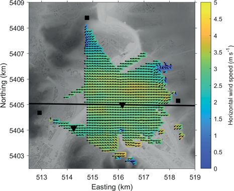
468            B. Adler et al.: Structures in the horizontal wind field over complex terrain       Meteorol. Z. (Contrib. Atm. Sci.)
                                                                                                                           29, 2020

probed height, not all cells travel with the same velocity           from different azimuthal directions. This method was
depending on their spatial dimensions, and the convec-               successfully applied over urban flat terrain (e.g. Cal-
tion velocity may not be constant with time (e.g. Pow-               houn et al., 2006) and over urban mountainous terrain
ell and Elderkin, 1974; Del Álamo and Jiménez,                       (Wittkamp et al., submitted). A third possible config-
2009). Using an array of tower measurements, Han et al.              uration is to perform coplanar (near)-horizontal plan-
(2019) studied the influence of the convection veloc-                position-indicator (PPI) scans with two or more Doppler
ity on the applicability of Taylor’s hypothesis in es-               lidars which allows the spatial distribution of the hor-
timating the streamwise length scale of structures in                izontal wind field to be retrieved. Already during the
the surface layer. They found that the global convec-                Joint Urban 2003 field campaign in Oklahoma City, Ok-
tion velocity is approximately 16 % larger than the mean             lahoma, dual-Doppler lidar scans were successfully used
streamwise velocity component at the same height and                 to study the horizontal wind field and structures in the
that the values of the streamwise length scale obtained              ABL over urban flat terrain for short time periods of a
from Taylor’s hypothesis agrees better with the values               few hours (Newsom et al., 2005; Newsom et al., 2008).
of the streamwise length scale obtained from spatially-              Träumner et al. (2015) used dual-Doppler lidar mea-
separated measurements when the convection velocity                  surements over flat horizontally heteorogeneous terrain
is used instead of the mean streamwise velocity com-                 to statistically investigate turbulent structures and coher-
ponent. The uncertainty arising from slight changes of               ence in the horizontal wind field in the surface layer for
the convection velocity can even explain some of the                 a time period of around 300 h. They calculated stream-
differences in turbulence parameters in the convective               and crosswise integral length scales and analyzed them
ABL calculated from temporal Doppler lidar measure-                  for situations with different atmospheric stratification. A
ments and spatial aircraft measurements (Adler et al.,               sequence of coplanar RHI and PPI scans performed with
2019). Unless an array of multiple 100-m towers can be               three scanning Doppler lidars was used by Haid et al.
installed, tower measurements can only be used to de-                (2020) to study the interaction between a cold pool and
duce the convection velocity in the surface layer. This              foehn over the city of Innsbruck in the Inn Valley, Aus-
is not only very expensive, but may even be impossible               tria. From the three described configurations, coplanar
over complex topography such as cities or mountainous                horizontal scans provide the horizontal wind field with
terrain. In order to get information on the convection ve-           the highest spatial and temporal resolution, however at
locity of cells in the middle and upper part of the ABL              the expense of information on the vertical structure of
or over highly complex terrain, another type of measure-             the horizontal wind field.
ment is thus necessary to provide simultaneous measure-                  Coplanar horizontal Doppler lidar measurements
ments at several locations in space with a high temporal             were conducted in Stuttgart in summer 2018 within the
resolution allowing the convective cells to be resolved.             framework of the Urban Climate Under Change [UC]2
    Combining measurements from several Doppler li-                  program. The program aims to develop and evaluate
dars is a promising approach to investigate both of the              a new building-resolving urban climate model for en-
above described topics, i.e. the mesoscale variability of            tire city regions and to test its practicability and usabil-
the flow over complex terrain and the displacement of                ity in collaboration with stakeholders (Scherer et al.,
cells in the convective ABL, as they can provide simulta-            2019b). To this purpose, high-quality three-dimensional
neous wind measurements at many locations (separated                 observational data were collected in three major Ger-
by several tens of meters) in a large area (few square               man cities, one of them being Stuttgart (Scherer et al.,
kilometers) which are not accessible by traditional in               2019a). Stuttgart is a city in moderate mountainous ter-
situ measurements, e.g. above buildings. As a Doppler                rain in south-western Germany which frequently suffers
lidar can only measure the radial velocity along the line-           from air quality issues. The orography is characterized
of-sight, the combination of two or more lidars is one               by a basin-shaped valley (Stuttgart basin) which opens
possible approach to get information on the wind vec-                into the Neckar Valley in the north-east (Figure 1a).
tor. One possible configuration is to perform coplanar               This complex topography makes Stuttgart an excellent
vertical range height indicator (RHI) scans with several             location in which to study the interactions between pro-
lidars and to retrieve the two-dimensional wind field in             cesses on different scales such as convection and ther-
the overlapping area (e.g. Newsom et al., 2008). This ap-            mally driven circulations. Using coplanar Doppler lidar
proach provides the two-dimensional wind vector in a                 measurements from 22 days in July and August 2018
vertical plane and was e.g. used to study intrusions and             together with additional in situ and remote sensing data,
waves in a Meteor crater basin in Arizona (Whiteman                  the following research questions are addressed in this
et al., 2018a; Whiteman et al., 2018b), to study wakes               study:
related to a wind energy turbine between two parallel
mountain ridges (Wildmann et al., 2018; Menke et al.,                 1. Which mesoscale horizontal flow structures occur in
2019; Palma et al., 2019), or to analyze the cross-valley                the area characterized by the opening of the Stuttgart
circulation in a major Alpine valley (Adler et al., sub-                 basin and the Neckar Valley? How regularly do these
mitted). Another approach is to retrieve horizontal wind                 structures occur? How do they depend on atmo-
profiles with so-called virtual towers by performing si-                 spheric stratification and the wind above the mean
multaneous measurements of the same volume of air                        ridge height?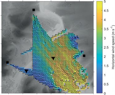
Meteorol. Z. (Contrib. Atm. Sci.)              B. Adler et al.: Structures in the horizontal wind field over complex terrain   469
29, 2020

                                                                        2. Is it possible to trace convective cells in the con-
                                                                           vective ABL over complex terrain and to estimate
                                                                           the convection velocity using coplanar Doppler lidar
                                                                           measurements? How does the convection velocity re-
                                                                           late to the mean horizontal wind speed?
                                                                        The paper is outlined as follows: in Section 2, the inves-
                                                                        tigation area, instrumentation and the method to retrieve
                                                                        the horizontal wind field are described. Section 3 gives
                                                                        examples of the flow characteristics and Section 4 con-
                                                                        tains a statistical analysis of the mesoscale flow struc-
                                                                        tures including the dependency on the ambient condi-
                                                                        tions. In Section 5, the displacement of convective cells
                                                                        is investigated and the method to derive the convection
                                                                        velocity is described. A summary and conclusions are
                                                                        given in Section 6.

                                                                        2 Measurement setup and data
                                                                          processing
                                                                        2.1 Investigation area
                                                                        The investigation area in Stuttgart is characterized by a
                                                                        basin-shaped valley called Stuttgart basin with a hor-
                                                                        izontal dimension of around 3 km × 3 km (Figure 1a).
                                                                        The Stuttgart downtown area is located in this basin.
                                                                        In the south-west, the basin is joined by the Nesenbach
                                                                        Valley and in the north-east, it opens into the Neckar
                                                                        Valley. The Neckar Valley roughly extends from the
                                                                        south-east to the north-west and is around 2 km wide.
                                                                        Besides these main characteristics, several smaller-scale
                                                                        orographic features such as side valleys and plateaus ex-
                                                                        ist in the area. The mean height of the surrounding ridges
                                                                        is at around 520 m above mean sea level (MSL) which is
                                                                        about 170 to 270 m above the valley floor. The Stuttgart
                                                                        basin and the Neckar Valley are both heavily built-up
                                                                        with residential and industrial areas. The local sum-
                                                                        mer time in Stuttgart is UTC plus 2 h and mean sunrise
                                                                        and sunset during the investigated period (21–29 July
                                                                        2018, 16–28 Aug 2018) are at around 04:10 UTC and
Figure 1: (a) Topographic height (terrain plus building height) in      18:45 UTC, respectively. In July and August 2018, five
the investigation area with instrument locations. Buildings within      remote sensing devices, all part of the mobile observa-
the city limits of Stuttgart are indicated in gray. Squares indicate    tion platform KITcube operated by Karlsruhe Institute
the locations of the scanning lidars #1, #2 and #3, respectively;       of Technology (Kalthoff et al., 2013), were deployed
circles mark the location of the surface station in Böblingerstraße     in the area (Kiseleva et al., 2019).
in the Nesenbach Valley (SB) and the location of the town hall in
the Stuttgart basin (ST); the triangles SO and NV indicate the points   2.2 Coplanar Doppler lidar measurements
at the opening of the Stuttgart basin into the Neckar Valley and in
the Neckar Valley, respectively, at which the retrieved horizontal          and retrieval of the horizontal wind field
wind field is analyzed in detail. (b) Topographic height and markers
like in (a), but with the PPI sectors scanned by lidars #1 (black),
                                                                        In order to use coplanar horizontal Doppler lidar scans
#2 (blue) and #3 (cyan) taking into account beam blocking by the        to study the spatio-temporal variability of the flow field,
topography. Each dot indicates one range gate. (c) Topographic          strict conditions and requirements must be met by the
height and markers like in (a), but with the distance Δz of the         experimental setup. Ideally, the lidars should be installed
lidar scanning plane above the topography at each grid point of         at the same height above mean sea level, have an unob-
the Cartesian retrieval grid. Only grid points where the intersection   structed view of the overlapping area and perform the
angle criteria is fulfilled are displayed. Coordinate system: UTM       PPIs at 0° elevation angle, which has the advantage that
(ETRS89) zone 32U.                                                      the measured radial velocity is purely a projection of the
                                                                        horizontal wind without any contributions by the vertical
                                                                        wind. The range gate lengths of the individual lidars, the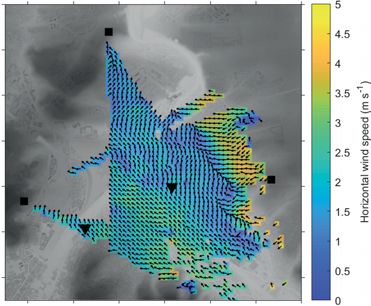
470            B. Adler et al.: Structures in the horizontal wind field over complex terrain               Meteorol. Z. (Contrib. Atm. Sci.)
                                                                                                                                   29, 2020
                                                                                                                     √
angular resolution of the PPI scans and the spacing of               are assigned within a certain radius R = Δl/ 2 of the
the grid on which the horizontal wind field is evaluated             grid point and the intersection angle of the individual li-
have to be fine enough to resolve the required spatial               dar beams is calculated. A system of N linear equations
scales. The lidars have to perform synchronized sweeps,              results at each grid point, with N being the number of ra-
i.e. they have to start and stop each PPI at the same time,          dial velocity measurement values that fall within R. This
and the time required for each PPI scan has to be short              system is solved by minimizing its cost function
enough to capture the temporal variability of the flow
field.
                                                                                                N

    These requirements were taken into account when                                        J=         (rvn − r̂n · vh )2              (2.2)
                                                                                                n=1
installing three Doppler lidars “Windcube 200s” manu-
factured by Leosphere in Stuttgart. They were placed on              and the most probable horizontal wind components are
three opposing slopes (Figure 1a): lidar #1 (363 m MSL)              deduced. A more detailed description of the retrieval
was installed on the grounds of the German Weather Ser-              method is e.g. given by Haid et al. (2020) and the Python
vice (DWD) at Schnarrenberg, lidar #2 (381 m MSL)                    code of the algorithm is available at GitHub (Haid,
in a vineyard owned by the city of Stuttgart and li-                 2019). Before solving Eq. 2.2, the radial velocity mea-
dar #3 (351 m MSL) on the grounds of the wine estate                 surements are filtered for outliers applying a threshold
Wöhrwag. Due to the challenge to find suitable measure-              filter to the carrier-to-noise ratio of -30 dB and a veloc-
ments sites, the lidars were not all at exactly the same             ity jump filter of 2 m s−1 to identify rapid, unrealistic
height above sea level, but had an offset of up to 30 m.             changes at each range gate for successive time stamps
The average height of the scanned plane was defined as               (1 s increments). The horizontal wind components are
365 m MSL, which is on average about 62 m above the                  rejected for grid points which do not fulfill the inter-
underlying topography (Figure 1c) and about half way                 section angle criteria: the intersection angle has to be
up the slopes. The sectors of the conducted PPI scans                between 30° and 150° for at least two of the lidars to
were limited by the topography, which e.g. prevented li-             avoid too large propagation errors, following the sug-
dar #1 to scan at azimuth angles larger than 180° (Fig-              gestions and considerations by Stawiarski et al. (2013)
ure 1b). All three lidars are identical in construction and          and Träumner et al. (2015). The largest possible area
were operated with the same technical specifications.                at which the horizontal wind field can be retrieved cov-
A physical range gate resolution of 50 m (laser pulse                ers several square kilometers (about 5 km × 5 km) (Fig-
length 200 ns) and no overlapping range gates resulted               ure 1c). The constraints by the intersection angle pre-
in a maximum theoretical measurement range of 100                    vent the retrieval in a substantial part of the opening
to 7200 m with 143 range gates. The accumulation time                of the Stuttgart basin into the Neckar Valley. The area
was set to 1 s and each PPI scan lasted for 60 s. As the             is further limited by the actual measurement ranges of
azimuth sector was 60° for all lidars, the angular resolu-           the lidars, which is usually lower during the day than
tion was 1°. The PPI scans were started synchronously                during the night, as visible in the horizontal wind field
every minute for all three lidars using the “Scheduler”              examples in Figure 2. The larger measurement ranges
option of the manufacturer software “Windforge” (ver-                during the night could be related to higher backscatter
sion 3.1.1). The synchronization accuracy of the start               due to a higher aerosol concentration when pollutants
times was around 0.35 s on average for all investigated              get trapped within the nocturnal surface inversion layer
days.                                                                or due to higher relative humidity values during night-
    Every minute, a set of three horizontal PPI scans was            time resulting in the growth of hygroscopic aerosols
obtained, which is used for the retrieval of the horizontal          (e.g. Veselovskii et al., 2009).
wind field. At 0° elevation angle, the radial velocity, rv,
measured by a Doppler lidar is a projection of the two-              2.3 Additional instrumentation
dimensional horizontal wind vector, vh = (u, v)T :
                                                                     In addition to the scanning “Windcube 200s” Doppler
            rv = r̂ · vh = u sin(az) + v cos(az)            (2.1)
                                                                     lidars, a fourth vertically profiling Doppler lidar “Wind-
with the two-dimensional unit vector in the direction of             cube WLS8-3" also manufactured by Leosphere was in-
the lidar beam, r̂, and the azimuth angle, az. In order              stalled on the roof top of the town hall (ST in Figure 1a)
to solve Eq. 2.1, at least two radial velocity measure-              at 325 m MSL in the Stuttgart basin. It provided horizon-
ments at the same point in space and time with different             tal wind profiles with the Doppler beam swinging (DBS)
azimuth angles have to be available. The radial veloc-               technique in a vertical range between 40 to 600 m above
ity measurements from the PPI scans are neither per-                 the device with an averaging interval of 10 min. The
fectly simultaneous nor exactly collocated. Because of               DBS technique is based on the assumption of horizontal
this, the horizontal wind vector is retrieved on a Carte-            homogeneity which may not be given over complex ter-
sian grid with a lattice length Δl = 100 m spanning the              rain. This can induce errors in the horizontal wind speed
horizontal scanning plane. The maximum temporal off-                 in the order of 10 % (Bingöl et al., 2009).
set at an arbitrary grid point is given by the scan du-                  Information on the atmospheric stratification was
ration of 60 s. To each grid point of the Cartesian grid,            obtained with a microwave radiometer “HATPRO-G4"
radial velocity measurement values from all three lidars             manufactured by Radiometer Physics GmbH, which was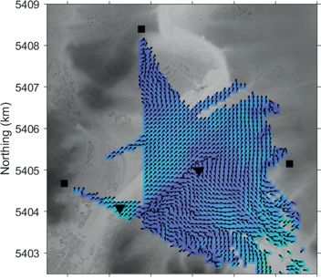
Meteorol. Z. (Contrib. Atm. Sci.)            B. Adler et al.: Structures in the horizontal wind field over complex terrain          471
29, 2020

       (a) 21:00                               (b) 01:18                                (c) 05:27

       (d) 19:38                               (e) 19:48                                (f) 20:02

       (g) 13:05                               (h) 13:07                                (i) 13:10

       (j) 13:05                               (k) 13:07                                 (l) 13:10

Figure 2: Examples of horizontal wind fields observed during different periods: horizontal wind speed (color-coded) and vector (arrows)
during nocturnal stable conditions at (a) 21:00 UTC, (b) 01:18 UTC and (c) 05:27 UTC; during the transition between convective and stable
conditions at (d) 19:38 UTC, (e) 19:48 UTC and (f) 20:02 UTC; and during daytime convective conditions at (g) 13:05 UTC, (h) 13:07 UTC
and (i) 13:10 UTC. The horizontal divergence fields corresponding to the horizontal wind fields shown in (g)–(i) is displayed in (j)–(l).
The example in (a) is on 23 July, the examples in (b)–(l) are on 24 July. Grey shading shows the topographic height, squares indicate the
locations of lidars #1, #2 and #3 and the triangles mark the points SO and NV, respectively (see Figure 1a).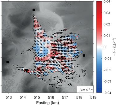
472            B. Adler et al.: Structures in the horizontal wind field over complex terrain       Meteorol. Z. (Contrib. Atm. Sci.)
                                                                                                                           29, 2020

installed on the tower of the town hall (ST in Figure 1a)                Another interesting flow feature is observed in the
at 357 m MSL in the Stuttgart basin. The retrievals to               evening towards the end of the example period (Fig-
obtain temperature profiles from the measured bright-                ure 2d–f). In the western part of the Neckar Valley, the
ness temperature are created with software provided by               horizontal wind is rather weak (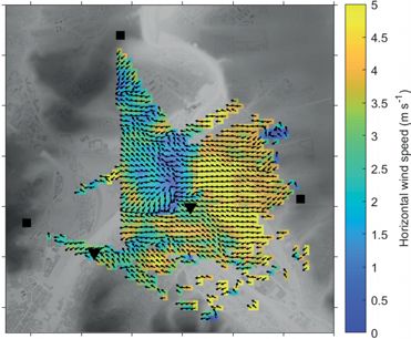
Meteorol. Z. (Contrib. Atm. Sci.)             B. Adler et al.: Structures in the horizontal wind field over complex terrain            473
29, 2020

Figure 3: Time series of the absolute frequency distribution (number of days for which the wind direction is within a 10 min × 10° bin) of
the wind direction below the mean ridge height in (a) the Neckar Valley (NV), (b) the opening of the Stuttgart basin (SO), (c) the Stuttgart
basin (ST) and (d) the Nesenbach Valley (SB) based on the horizontal wind data of all 22 available days. The height above the topography
at which the measurements were taken are indicated in brackets. To make the wind directions at NV and SO, which are retrieved from the
coplanar Doppler lidar scans, comparable to the data from the wind profiling lidar (ST) and the surface station (SB), the wind direction
at NV and SO are averaged over 10 min before calculating the frequency distribution. Dashed and solid lines indicate up- and downvalley
direction in (a), (c) and (d) and in- and outflow direction in (b), respectively.

4 Statistics of mesoscale flow structures                              Neckar Valley, at the opening and in the Stuttgart basin
                                                                       was around 80–90 m above the underlying topography,
4.1 Frequency distribution of the wind                                 while the measurements in the Nesenbach Valley were
                                                                       taken at 10 m above the ground. This means that all mea-
    direction
                                                                       surements were taken well below the mean ridge height.
The individual horizontal wind fields (Figure 2) from                  The absolute frequency distribution of the wind direc-
the example in Section 3 indicate that different types of              tion at the four locations is calculated for all 22 days
flow regimes occur on the mesoscale depending on the                   (Figure 3).
time of the day and location. To get a statistical view                    From the late morning until the early evening, the
of the flow conditions below the mean ridge height, the                wind direction is rather scattered at all locations, with a
horizontal wind direction is evaluated at four locations:              slight preference for a northerly flow component (Fig-
one in the Neckar Valley (NV in Figure 1a) and one in                  ure 3).
the opening of the Stuttgart basin into the Neckar Val-                    During the night and morning hours, distinct differ-
ley (SO). In addition, the horizontal wind direction at                ences are evident at the individual sites, which are in-
405 m MSL measured with the profiling lidar on the roof                line with the orographic structures. In the northwest-
top of the town hall in the Stuttgart basin (ST) and at                southeast oriented Neckar Valley (Figure 3a), south-
the surface station at Böblingerstraße (SB) is analyzed                easterly flow clearly dominated during nighttime and
statistically to extend the investigation of the flow char-            in the early morning until around 08:30 UTC, which
acteristics into the Stuttgart basin and the Nesenbach                 corresponds to a downvalley wind. In the Stuttgart
Valley. The measurement height at the locations in the                 basin (Figure 3c) and in the Nesenbach Valley (Fig-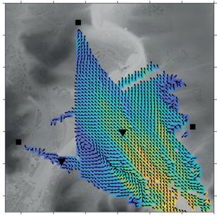
474            B. Adler et al.: Structures in the horizontal wind field over complex terrain       Meteorol. Z. (Contrib. Atm. Sci.)
                                                                                                                           29, 2020

ure 3d), the dominant wind direction during the night                when the wind above the mean ridge height comes from
(around 20:00 UTC to 06:00 UTC) is south-westerly and                the south-westerly to north-westerly sector, i.e. 250° and
southerly, respectively. This indicates downvalley wind              330° (Figure 4b, e, h). For these cases, the wind direction
flowing out of the Nesenbach Valley into the Stuttgart               below ridge is slightly turned counter-clockwise, i.e. the
basin following the shape of the terrain (Figure 1a).                values lie below the diagonal. Independent of the wind
   At the opening of the Stuttgart basin into the Neckar             direction above the mean ridge height, south-easterly
Valley, two wind directions prevail during the night                 downvalley wind is another common wind direction in
and morning hours (Figure 3b): from around 20:30 to                  the Neckar Valley for this stability regime (Figure 4b).
05:00 UTC south-westerly flow dominates, indicating                  This means that the flow in the valley is decoupled from
an outflow of the basin into the Neckar Valley. After                the flow aloft, although the BRN values indicate dy-
around 05:00, north-easterly flow becomes more promi-                namically unstable conditions. Due to the orientation
nent, which is equivalent with an inflow into the basin              of the valley axis in the Stuttgart basin, it is not possi-
from the Neckar Valley. The flow field in Figure 2c is               ble to make this distinction in the Stuttgart basin (Fig-
an example for such a flow condition from which it                   ure 4h). For BRN > 1.25, i.e. dynamically stable condi-
seems likely that the inflow into the basin is related to            tions, the flows in the Neckar Valley (Figure 4c) and in
the downvalley wind in the Neckar Valley which pushes                the Stuttgart basin (Figure 4i) have a clear preference for
through the opening into the basin.                                  downvalley direction, i.e. south-easterly in the Neckar
                                                                     Valley and south-westerly in the Stuttgart basin.
4.2 Dependency of the flow below the mean                                At the opening of the Stuttgart basin, the preferred
    ridge height on the flow aloft and                               wind directions during thermally stable conditions are
    atmospheric stratification                                       north-easterly, which indicates an inflow, and south-
                                                                     westerly, which indicates an outflow (Figure 3e, f). The
In the next step, the relationship between the wind direc-           two flow regimes are most pronounced during dynami-
tion below the mean ridge height at three different loca-            cally stable conditions (Figure 3f).
tions (in the Stuttgart basin (ST), at the opening (SO)
and in the Neckar Valley (NV)) and the wind direction                4.3 Discussion and interpretation
above the mean ridge height and atmospheric stratifica-
tion is investigated. We follow the approach described               During convective conditions the wind direction be-
by Wittkamp et al. (submitted) who investigated the                  low and above the mean ridge height are similar at all
same relationship during summer 2017. Instead of using               sites (Figure 4a, d, g), which indicates that both lay-
coplanar horizontal scans, these authors retrieved wind              ers are coupled due to turbulent mixing in the convec-
direction profiles at the opening of the Stuttgart basin             tive ABL. A slight preference for a northerly flow com-
and in the Neckar Valley with the virtual tower method.              ponent is visible (Figs. 3 and 4a, d, g). Given the ori-
In our study, the ambient horizontal wind, i.e. the wind             entation of the valleys (Figure 1a), north-westerly flow
above the mean ridge height, is defined as the horizon-              in the Neckar Valley (Figure 3a), north-easterly flow
tal wind measured at 705 m MSL with the profiling li-                in the Stuttgart basin (Figure 3c) and northerly flow
dar and the Bulk-Richardson number (BRN) is calcu-                   in the Nesenbach Valley (Figure 3d) indicate upvalley
lated using horizontal wind and temperature information              wind. Besides the upvalley wind, south-westerly wind
at two heights (405 and 685 m MSL) from the profil-                  sometimes occurs in the Nesenbach Valley during the
ing lidar and the microwave radiometer located at ST in              day (Figure 3d) which could be related to large-scale
the Stuttgart basin. Wittkamp et al. (submitted) found a             driven channeling (Whiteman and Doran, 1993). The
critical BRN value of 1.25 which separated dynamically               slightly counter-clockwise turned wind direction below
unstable cases (BRN < 1.25), during which the flow in                the mean ridge height for dynamically unstable condi-
the valleys was coupled to the flow aloft and dynami-                tions (Figure 4b,e,h) could be related to the impact of
cally stable cases (BRN > 1.25), during which the flow               surface friction on the flow below the mean ridge height,
was decoupled and mainly directed in downvalley direc-               which becomes relevant as vertical mixing is lower in
tion. In our study, around 2500 10-min periods are avail-            this regime than during convective conditions. This is
able for the analysis during the 22 investigated days,               in agreement with the Ekman spiral theory (e.g. Stull,
which are nearly equally distributed over three BRN                  1988) and is also found by Wittkamp et al. (submitted).
regimes, i.e. BRN < 0, 0 ≤ BRN < 1.25, BRN ≥ 1.25. Our                   Cases with coupled flows (wind direction below and
sample size is thus much larger than the one available               above the mean ridge height are similar) and uncoupled
during summer 2017 and presented in Wittkamp et al.                  flows (downvalley wind independent of the wind direc-
(submitted).                                                         tion above the mean ridge height) are both found in the
    During convective conditions (BRN < 0), wind di-                 Neckar Valley for dynamically unstable conditions (Fig-
rection below and above the mean ridge height match,                 ure 4b). Both cases are scattered throughout the whole
i.e. the values lie on or near the diagonal for many of              range of BRN values (between 0 and 1.25). This means
the cases (Figure 4a, d, g). During dynamically unsta-               that changing the BRN thresholds to define the dynam-
ble conditions (0 ≤ BRN < 1.25), wind direction below                ically unstable regime does not allow to better distin-
and above the mean ridge height are also often similar               guish between both cases. One possible reason for this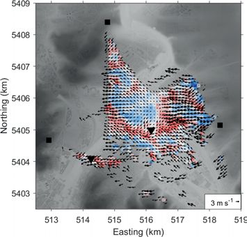
Meteorol. Z. (Contrib. Atm. Sci.)             B. Adler et al.: Structures in the horizontal wind field over complex terrain           475
29, 2020

Figure 4: Relationship between the wind direction above the mean ridge height at 705 m MSL and the wind direction below the mean ridge
height at 365 m MSL in (a, b, c) the Neckar Valley (NV) and (d, e, f) the opening of the Stuttgart basin (SO) and at 405 m MSL (g, h, i)
in the Stuttgart basin (ST). The data are separated according to the BRN regimes: (a, d, g) BRN < 0, (b, e, h) 0 ≤ BRN < 1.25 and (c, f, i)
BRN ≥ 1.25. The color code shows the number of days for which the wind direction is within a 10° × 10° bin. The wind components at NV
and SO, which are retrieved from the coplanar Doppler lidar scans, are averaged over 10-min periods before calculating the wind direction.
Dashed and solid horizontal lines indicate up- and downvalley direction at NV and ST and in- and outflow direction at SO, respectively.

could be that the conditions in the Stuttgart basin, where             ing nighttime and an inflow preferentially occurs during
BRN is calculated, are not representative for the condi-               the morning hours. There is no clear dependency of both
tions in the Neckar Valley during these cases. Another                 flow regimes on the wind direction above ridge level, al-
reason could be the uncertainty related to the BRN cal-                though a slight preference of outflow with ambient west-
culation as both the temperature profiles measured by                  erly wind might exist (Figure 4e, f).
the microwave radiometer and the horizontal wind pro-
files from the profiling lidar are subject to errors related
to the measurement techniques.                                         5 Displacement of structures in the
    Based on the BRN values, it is not possible to distin-               convective ABL
guish between inflow and outflow cases at the opening of
the Stuttgart basin (Figure 4e, f). This could be related to           During daytime, the movement of structures character-
the same reasons as above, i.e. the non-representativity               ized by enhanced and reduced horizontal wind speed
of the BRN values for the conditions at the opening                    is often detected on the 22 investigated days (example
and the uncertainty of the BRN calculation. The diur-                  in Figure 2g–i) and we relate these structures to con-
nal cycle of wind direction at the opening (Figure 3b),                vective cells which move through the ABL with a cer-
however, indicates that an outflow is more likely dur-                 tain convection velocity. Sophisticated methods to track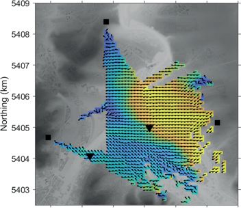
476 B. Adler et al.: Structures in the horizontal wind field over complex terrain Meteorol. Z. (Contrib. Atm. Sci.)
29, 2020
structures in time and space have been developed in
the past (e.g. Handwerker, 2002). Based on the cal- (a)
culation of the spatial cross-correlation between subse-
quent images of the horizontal wind field, Duncan Jr
et al. (2019) proposes a method to estimate the speed
with which structures move downwind. However, their
method relies on a well resolved wind field and a large
data availability within the measurement domain. Data
availability during daytime is often limited by the maxi-
mum measurement ranges of the lidars during daytime, NV
which may lead to only partial resolution of the con-
vective cells. Such a method based on the spatial cross-
correlation is thus not applicable to our data.
5.1 Method to estimate the convection velocity
To estimate the convection velocity, we therefore use the (b)
following method which works well with the imposed
restrictions. We first estimate the mean wind direction
for a 60-min period by temporally and spatially averag-
ing the horizontal wind components. Figure 5a shows
an example of the spatial distribution of the temporally
averaged horizontal wind field. A line along the mean
wind direction is then placed through the location in the
Neckar Valley (NV). This location was chosen as it was
often near the center of the area where the horizontal
wind retrieval provided data. For every individual hor-
izontal wind field within the 60-min period, the hori-
zontal wind speed values along this line are extracted.
An example of the resulting time distance plot of hor-
izontal wind speed is shown in Figure 5b. To enhance
the number of 60-min periods available for the analy-
sis, gaps of less than 10 pixels (size of one pixel is
100 m × 100 m) in the time distance plots are linearly in-
terpolated. For example, one pixel missing for 10 min or
a gap of 1000 m during one time stamp are interpolated.
The number of interpolated pixels is less than 1 % on
the average. The displacement of structures with time is
clearly visible as the elongated streaks with low and high
horizontal wind speed. The slope of each streak repre-
sents the convection velocity of the corresponding cell.
Instead of calculating the slope of each streak manually
by hand, we estimate a global convection velocity for Figure 5: (a) Mean horizontal wind field averaged for the time pe-
riod 13:00 to 14:00 UTC on 24 July. The black straight line indicates
the 60-min period. To this purpose, the two-dimensional
the mean wind direction of 91° which results when averaging the
auto-correlation function is calculated for the 60-min wind components over space and time for the 60-min period. Grey
time distance plot (Figure 5b, 6). From the slope a of shading shows the topographic height. (b) Time distance plot of the
the fit horizontal wind speed along the straight line from (a) through the
location NV in the Neckar Valley for the corresponding time period.
lt = a · ld (5.1) In (b), crosses indicate pixels where the values are linearly interpo-
lated.
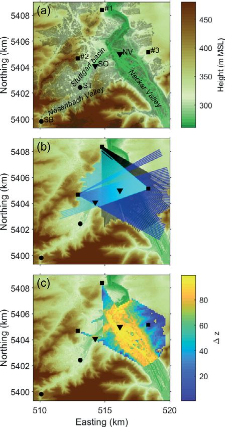
to the elongated shape of positive auto-correlation the
convection velocity vc is estimated as
vc = |a|−1 (5.2) done by Pantillon et al. (2020) who applied the two-
dimensional auto-correlation function to a time distance
using only pixels where the auto-correlation function is plot of radial velocity measured by single lidar during
larger than 0.5. lt denotes the lag in time and ld the rapid low-elevation RHI scans to investigate coherent
lag in distance. This method can also be applied to structures related to cyclonic winter storms.
radial velocity measured by a single lidar when the beam If the availability of data in the 60-min time dis-
is pointed in the mean wind direction. This was e.g. tance plot is too small or the fit to the two-dimensionalMeteorol. Z. (Contrib. Atm. Sci.) B. Adler et al.: Structures in the horizontal wind field over complex terrain 477
29, 2020
to 3.0 m s−1 . As the mean horizonal wind speed stays the
same, the convection velocity is then only 20 % higher
than the mean wind speed.
It is rather likely that the movement of the cells is
controlled by the horizontal wind speed in a certain
height in the ABL. This steering level presumably de-
pends on the vertical extent of the convective cells. Thus,
individual cells may travel with a different speed, as they
are steered by the flow at different levels depending on
their vertical extent. With the method described in Sec-
tion 5.1 we obtain a global convection velocity for all
types of structures within each 60-min period, which
does not take into account the movement of individual
cells.
The lidar scanning plane is at 365 m MSL, i.e. 62 m
above the topography on the average (Figure 1c). This
Figure 6: Two-dimensional auto-correlation function, r, of the time means that it is still in the lower part of the ABL and
distance plot of the horizontal wind speed shown in Figure 5b. Only probably in the transition zone between the surface layer
pixels with an auto-correlation larger than 0.5 (black dots) are used and the mixed layer. As evident in the mean horizon-
for the fit (black line). From the slope of the linear fit, the convection tal wind profile calculated for the corresponding pe-
velocity, vc , is determined if the coefficient of determination, R2 , is riods from the profiling Doppler lidar in the Stuttgart
higher than 0.5. basin, horizontal wind speed in the ABL increases with
height up to around 600 m MSL and stays roughly con-
stant above (not shown). This is likely due to the sur-
auto-correlation function fails, the estimated convection face roughness induced by the buildings and terrain. The
velocity is not reasonable. Consequently, the convec- height at which the mean horizontal wind speed agrees
tion velocity is disregarded when the dimensions of the with the mean convection velocity of 3.1 m s−1 is at
horizontal wind speed field are less than 50 × 10 pix- around 465 m MSL, i.e. 100 m above the lidar scanning
els, which corresponds to 50 min in time and 1000 m in plane. Although the scatter is larger and the coefficient
space, or when the coefficient of determination of the fit of determination is smaller (R2 = 0.51) when comparing
is less than 0.5. Possible reasons for the fit to fail can the convection velocity with the horizontal wind speed
be that simply no streaks are visible in the time distance at 465 m MSL (Figure 7b) instead of at 365 m MSL (Fig-
plot as no convective cells propagate with the mean wind ure 7a), it is evident that the values lie closer around the
or that the wind direction changes substantially within bisectrix (slope of the line of best fit is 0.95) in Figure 7b
the 60-min period. than in Figure 7a. This means that the speed with which
the convective cells detected at 365 m MSL overall move
5.2 Relationship between the horizontal wind is closer to the horizontal wind speed at 465 m MSL, i.e.
speed and convection velocity the cells movement is steered by the flow at this higher
level. The larger scatter in Figure 7b than in Figure 7a
The method described in Section 5.1 is applied to could be related to the uncertainties related to the hori-
all 22 days for the time period between 06:00 and zontal wind measurements by the profiling lidar and to
18:00 UTC. After applying the strict filter criteria, the spatial distance of a few kilometers between the pro-
83 60-min time periods remain. Figure 7a shows the filing lidar measurements in the Stuttgart basin and the
relationship between the mean horizontal wind speed coplanar lidar measurements in the Neckar Valley (Fig-
at 365 m MSL, i.e. at the height of the lidar scanning ure 1).
plane where the convection velocity is estimated, and the
convection velocity. While both values generally agree
quite well (R2 = 0.76), the mean convection veloc- 6 Summary and conclusions
ity is 0.6 m s−1 (24 %) higher than the mean horizon-
tal wind speed, vh , of 2.5 m s−1 . The line of best fit is The flow in the ABL over complex terrain is highly vari-
vh = 0.79 · vc . This means that the cells move faster than able in space and time. In order to capture the (sub-)
the mean flow at the same height, which is in agree- mesoscale characteristics of the flow by means of obser-
ment with the findings of Han et al. (2019). Note that vations, simultaneous measurements at many locations
this mean percentage value is quite sensitive to outliers. in space are necessary. In some distance above the sur-
When excluding four values for which the difference be- face or in complex or inaccessible terrain such as urban
tween the wind speed and the convection velocity dif- or mountainous areas, these kind of measurements can
fered more than twice the standard deviation from the realistically only be obtained with remote sensing in-
mean difference (values are indicated by the red out- struments. By performing synchronized horizontal co-
lines in Figure 7a) the mean convection velocity reduces planar scans with three Doppler lidars on 22 days in478 B. Adler et al.: Structures in the horizontal wind field over complex terrain Meteorol. Z. (Contrib. Atm. Sci.)
29, 2020
(a) (b)
Figure 7: Relationship between the convection velocity and (a) the mean horizontal wind speed at 365 m MSL determined from the temporal
and spatial average of the retrieved horizontal wind components for each 60-min period and (b) the horizontal wind speed at 465 m MSL
measured by the profiling lidar at ST. The convection velocity is estimated with the method described in Section 5. The solid line indicates
the bisectrix and the dashed line shows the line of best fit, vh = a · vc . The coefficient of determination, R2 , the slope of the line of best fit, a,
the mean horizontal wind speed, vh , and the mean convection velocity, vc are given. The red outlines in (a) indicate outlier values (for
details see text).
summer 2018 within the [UC]2 program, we retrieved The large spread is likely related to the moderate
the horizontal wind field in a horizontal plane of several valley depths of around 200 m in which thermally
square kilometers above the city of Stuttgart. The terrain driven circulations are less pronounced and masked
around Stuttgart is characterized by a basin-shaped val- during daytime by convection compared to deeper
ley (Stuttgart basin) which is joined by the Nesenbach valleys.
Valley and opens into the larger Neckar Valley. The hor-
2. Convective cells which propagate downstream are
izontal wind field is available every 60 s and has a hori-
detected during daytime in the horizontal wind field.
zontal resolution of 100 m. This study pursues two main
When plotting the horizontal wind speed extracted
objectives: (1) to identify the mesoscale flow structures
along the line of the mean wind direction against time
in the valleys and to investigate how often they occur
for 60-min periods, elongated streaks are visible. The
and how they depend on the flow above the mean ridge
slope of each streak gives the speed with which the
height and on atmospheric stratification and (2) to detect
cell propagates downstream, i.e. the convection ve-
and trace convective cells which move through the ABL
locity. This velocity is relevant when temporal point
and to estimate the convection velocity.
measurements are transferred to space to investi-
1. During dynamically stable conditions, which are gate the spatial characteristics of the cells. By calcu-
identified by calculating the Bulk-Richardson num- lating the two-dimensional auto-correlation function
ber, the flow below the mean ridge height is regu- for each 60-min time distance plot, a global convec-
larly decoupled from the flow aloft and the wind di- tion velocity is obtained for all cells within each time
rection in the Neckar Valley, Nesenbach Valley and period. Comparing the convection velocity with the
Stuttgart basin reveals a clear preference for ther- mean horizontal wind speed at the height of the lidar
mally driven downvalley wind. At the opening of scanning plane at 365 m MSL (about 62 m above the
the Stuttgart basin into the Neckar Valley, two flow topography), i.e. the same level where the convec-
regimes are found, which are rather independent of tion velocity is calculated, reveals that the correlation
the wind direction above the mean ridge height. An between both velocities is quite good (R2 = 0.76),
outflow of the basin occurs mainly during the night- while the convection velocity is higher by 24 % on
time hours, while an inflow dominates in the morn- the average. This result, which is retrieved from mea-
ing. The switching between in- and outflow may surements over highly complex urban and mountain-
have important implications for the ventilation of the ous terrain, is in general agreement with the find-
Stuttgart basin and thus for the air-quality, which will ings of Han et al. (2019), whose results are based on
be investigated in future studies. tower measurements conducted over a dry flat bed of
During thermally unstable conditions, the flow below a lake.
and above the mean ridge height is mainly coupled, Using horizontal wind profiles obtained with a pro-
i.e. the wind direction is very similar. Although the filing lidar in the Stuttgart basin a few kilometers
wind direction varies a lot, a preference for northerly away from the area where the convection velocity
flow is evident, which is equivalent to upvalley wind. is estimated, we find that the global convection ve-Meteorol. Z. (Contrib. Atm. Sci.) B. Adler et al.: Structures in the horizontal wind field over complex terrain 479
29, 2020
locity is more similar to the horizontal wind speed team from IMK for instrument installation and conduct-
100 m above the lidar scanning plane. This suggests ing of the campaign. We also thank our project partners
that this is the overall steering level, which controls from DWD and the city of Stuttgart for providing the
the movement of the convective cells. This could be surface data measurements. Further we thank the DLR
further investigated with an experimental setup con- for topographic data and the city of Stuttgart, the wine
sisting of profiling measurements in the area of the estate Wöhrwag and DWD for allowing our instruments
coplanar horizontal scans and several sets of scan- on their grounds.
ning lidars which are installed at different heights on
slopes overlooking a valley deeper than the one tar-
geted here. This would allow to retrieve the convec-
Supplemental data
tion velocity at several levels throughout the ABL. The supplement data set (https://zenodo.org/record/
Such a setup might also give new insights into the 3901434#.XvBpd2gzabg) contains a 24-h movie
spatial characteristics of the flow in deeper valleys. (21:00 UTC 23 July to 21:00 UTC 24 July) of the
The vertical cross-valley flow structure in such val- horizontal wind field in a horizontal plane above the city
leys has recently been targeted by vertical coplanar of Stuttgart retrieved from coplanar horizontal Doppler
Doppler lidar measurements in the Inn Valley, Aus- lidar scans. The measurements were conducted within
tria, (Adler et al., submitted), but detailed measure- the framework of the Urban Climate under Change
ments of the horizontal flow structure with high [UC]2 program.
spatio-temporal resolution are still missing.
Our analysis demonstrates the benefit of area-wide References
measurements of the horizontal wind field with a high
spatial and temporal resolution in contrast to point mea- Adler, B., N. Kalthoff, 2014: Multi-scale transport pro-
cesses observed in the boundary layer over a mountainous is-
surements at individual sites which suffer from limited land. – Bound.-Layer Meteor. 153, 515–537, DOI: 10.1007/
representativeness in complex terrain. This kind of in- s10546-014-9957-8.
formation can only be achieved by measuring simulta- Adler, B., N. Kalthoff, 2016: The impact of upstream flow on
neously at the same point in space with at least two the atmospheric boundary layer in a valley on a mountainous
Doppler lidars. The third Doppler lidar used in this study island. – Bound.-Layer Meteor. 158, 429–452, DOI: 10.1007/
enlarges the area in which the horizontal wind field can s10546-015-0092-y.
be retrieved. With such spatial measurements it is e.g. Adler, B., O. Kiseleva, N. Kalthoff, A. Wieser, 2019: Com-
parison of convective boundary layer characteristics from air-
possible to detect and study the spatial variability and craft and wind lidar observations. – J. Atmos. Oceanic Tech-
diurnal cycle of the flow within a valley or at the conflu- nol. 36, 1381–1399, DOI: 10.1175/JTECH-D-18-0118.1.
ence of two valleys which is influenced by the interac- Adler, B., N. Kalthoff, O. Kiseleva, 2020: The diurnal cycle
tion of convection and thermally and dynamically driven of the horizontal wind field over complex terrain detected with
flows. Even vortices with a vertical axis or convective coplanar Doppler lidar scans. – Zenodo, published online,
cells can be visualized. One big issue when perform- DOI: 10.5281/zenodo.3901434.
ing point measurements at towers or with a profiling li- Adler, B., A. Gohm, N. Kalthoff, N. Babić, U. Corsmeier,
M. Lehner, M.W. Rotach, M. Haid, P. Markmann,
dar is often the representativity of the location. Spatial E. Gast, G. Tsaknaki, G. Georgoussis, submitted:
measurements performed with coplanar Doppler lidar CROSSINN – a field experiment to study the three-
scans could help to address the representativity and to dimensional flow structure in the Inn Valley, Austria. – Bull.
identify suitable locations. These types of measurements Amer. Meteor. Soc.
also open up new possibilities for model evaluation and Allwine, K.J., J.H. Shinn, G.E. Streit, K.L. Clawson,
may prove useful for air pollution studies and wind en- M. Brown, 2002: Overview of URBAN 2000: A multi-
ergy research. In future scenarios when drones are flying scale field study of dispersion through an urban environ-
ment. – Bull. Amer. Meteor. Soc. 83, 521–536, DOI: 10.1175/
over cities e.g. to deliver medicine or to monitor traffic 1520-0477(2002)0832.3.CO;2.
(Khan et al., 2018), real-time monitoring of the wind Barlow, J.F., 2014: Progress in observing and modelling the
field above cities, similar to the automatic wind shear urban boundary layer. – Urban Climate 10, 216–240, DOI:
detection performed at some airports (e.g. Chan et al., 10.1016/j.uclim.2014.03.011.
2006), will likely be relevant for a smooth and safe op- Bingöl, F., J. Mann, D. Foussekis, 2009: Conically scanning
eration. Coplanar Doppler lidar measurements might be lidar error in complex terrain. – Meteorol. Z. 18, 189–195,
the solution to that. DOI: 10.1127/0941-2948/2009/0368.
Calhoun, R., R. Heap, M. Princevac, R. Newsom, H. Fer-
nando, D. Ligon, 2006: Virtual towers using coherent
Doppler lidar during the Joint Urban 2003 dispersion exper-
Acknowledgments iment. – J. Appl. Meteor. Climatol. 45, 1116–1126, DOI:
10.1175/JAM2391.1.
Chan, P., C. Shun, K. Wu, 2006: Operational LIDAR-based
The German Federal Ministry of Education and system for automatic windshear alerting at the Hong Kong In-
Research (BMBF) funded the project under grant ternational Airport. – In: 12th Conference on Aviation, Range,
01LP1602 G within the research programme [UC]2 . We and Aerospace Meteorology, 6.11, Atlanta, GA. Amer. Me-
would like to thank Andreas Wieser and the whole teor. Soc.480 B. Adler et al.: Structures in the horizontal wind field over complex terrain Meteorol. Z. (Contrib. Atm. Sci.)
29, 2020
Crewell, S., U. Löhnert, 2007: Accuracy of boundary layer der Change’ [UC]2). – https://publikationen.bibliothek.kit.
temperature profiles retrieved with multifrequency multian- edu/1000093534, DOI: 10.5445/IR/1000093534.
gle microwave radiometry. – IEEE Transactions on Geo- Kossmann, M., R. Vögtlin, U. Corsmeier, B. Vogel,
science and Remote Sensing 45, 2195–2201, DOI: 10.1109/ F. Fiedler, H.J. Binder, N. Kalthoff, F. Beyrich, 1998:
TGRS.2006.888434. Aspects of the convective boundary layer structure over com-
Del Álamo, J.C., J. Jiménez, 2009: Estimation of turbu- plex terrain. – Atmos. Env. 32, 1323–1348, DOI: 10.1016/
lent convection velocities and corrections to Taylor’s ap- S1352-2310(97)00271-9.
proximation. – J. Fluid Mech. 640, 5–26, DOI: 10.1017/ Lareau, N.P., E. Crosman, C.D. Whiteman, J.D. Horel,
S0022112009991029. S.W. Hoch, W.O. Brown, T.W. Horst, 2013: The persis-
Duncan Jr, J.B., B.D. Hirth, J.L. Schroeder, 2019: Enhanced tent cold-air pool study. – Bull. Amer. Meteor. Soc. 94, 51–63,
estimation of boundary layer advective properties to improve DOI: 10.1175/BAMS-D-11-00255.1.
space-to-time conversion processes for wind energy applica- Löhnert, U., S. Crewell, 2003: Accuracy of cloud liquid water
tions. – Wind Energy 22, 1203–1218, DOI: 10.1002/we.2350. path from ground-based microwave radiometry 1. dependency
Gohm, A., F. Harnisch, J. Vergeiner, F. Obleitner, on cloud model statistics. – Radio Science 38, 8041. DOI:
R. Schnitzhofer, A. Hansel, A. Fix, B. Neininger, 10.1029/2002RS002654.
S. Emeis, K. Schäfer, 2009: Air pollution transport in an Löhnert, U., D. Turner, S. Crewell, 2009: Ground-based
Alpine valley: results from airborne and ground-based obser- temperature and humidity profiling using spectral infrared and
vations. – Bound.-Layer Meteor. 131, 441–463, DOI: 10.1007/ microwave observations. Part I: simulated retrieval perfor-
s10546-009-9371-9. mance in clear-sky conditions. – J. Appl. Meteor. Climatol.
Haid, M., 2019: marenha/doppler_wind_lidar_toolbox: First re- 48, 1017–1032, DOI: 10.1175/2008JAMC2060.1.
lease (v1.0.0). – https://zenodo.org/record/3583083 or the Menke, R., N. Vasiljević, J. Mann, J.K. Lundquist, 2019:
github repository https://github.com/marenha/doppler_wind_ Characterization of flow recirculation zones at the Perdigão
lidar_toolbox/tree/v1.0.0. DOI: 10.5281/zenodo.3583083. site using multi-lidar measurements. – Atmos. Chem. Phys.
Haid, M., A. Gohm, L. Umek, H.C. Ward, T. Muschinski, 19, 2713–2723, DOI: 10.5194/acp-19-2713-2019.
L. Lehner, M.W. Rotach, 2020: Foehn-cold pool interac- Newsom, R.K., D. Ligon, R. Calhoun, R. Heap, E. Cregan,
tions in the Inn Valley during PIANO IOP2. – Quart. J. Roy. M. Princevac, 2005: Retrieval of microscale wind and tem-
Meteor. Soc. 146, 728, DOI: 10.1002/qj.3735. perature fields from single- and dual-Doppler lidar data. –
Han, G., G. Wang, X. Zheng, 2019: Applicability of Taylor’s J. Appl. Meteor. 44, 1324–1345, DOI: 10.1175/JAM2280.1.
hypothesis for estimating the mean streamwise length scale of Newsom, R., R. Calhoun, D. Ligon, J. Allwine, 2008: Lin-
large-scale structures in the near-neutral atmospheric surface early organized turbulence structures observed over a subur-
layer. – Bound.-Layer Meteor. 172, 215–237, DOI: 10.1007/ ban area by dual-Doppler lidar. – Bound.-Layer Meteor. 127,
s10546-019-00446-3. 111–130, DOI: 10.1007/s10546-007-9243-0.
Handwerker, J., 2002: Cell tracking with TRACE3D-a Palma, J., A.S. Lopes, V.C. Gomes, C.V. Rodrigues,
new algorithm. – Atmos. Res. 61, 15–34, DOI: 10.1016/ R. Menke, N. Vasiljević, J. Mann, 2019: Unravelling the
S0169-8095(01)00100-4. wind flow over highly complex regions through computational
Jackson, P.L., G. Mayr, S. Vosper, 2013: Dynamically-driven modeling and two-dimensional lidar scanning. – In: Journal of
winds. – In: Chow, F.K., S.F. De Wekker, B.J. Snyder Physics: Conference Series, volume 1222, 012006. IOP Pub-
(Eds.): Mountain weather research and forecasting. – Springer lishing, DOI: 10.1088/1742-6596/1222/1/012006.
atmospheric sciences, Springer, Dordrecht, 121–218, DOI: Pantillon, F., B. Adler, U. Corsmeier, P. Knippertz,
10.1007/978-94-007-4098-3_3. A. Wieser, A. Hansen, 2020: Formation of wind gusts in an
Kalthoff, N., B. Vogel, 1992: Counter-current and chan- extratropical cyclone in light of Doppler lidar observations and
nelling effect under stable stratification in the area of Karl- large-eddy simulations. – Mon. Wea. Rev. 148, 353–375, DOI:
sruhe. – Theor. Appl. Climatol. 45, 113–126, DOI: 10.1007/ 10.1175/MWR-D-19-0241.1.
BF00866400. Powell, D.C., C. Elderkin, 1974: An investigation of the ap-
Kalthoff, N., H.J. Binder, M. Kossmann, R. Vögtlin, plication of Taylor’s hypothesis to atmospheric boundary layer
U. Corsmeier, F. Fiedler, H. Schlager, 1998: Temporal turbulence. – J. Atmos. Sci. 31, 990–1002, DOI: 10.1175/
evolution and spatial variation of the boundary layer over com- 1520-0469(1974)0312.0.CO;2.
plex terrain. – Atmos. Env. 32, 1179–1194, DOI: 10.1016/ Scherer, D., F. Ament, S. Emeis, U. Fehrenbach, B. Leitl,
S1352-2310(97)00193-3. K. Scherber, C. Schneider, U. Vogt, 2019a: Three-
Kalthoff, N., B. Adler, A. Wieser, M. Kohler, K. Träum- dimensional observation of atmospheric processes in cities. –
ner, J. Handwerker, U. Corsmeier, S. Khodayar, D. Lam- Meteorol. Z. 28, 121–138, DOI: 10.1127/metz/2019/0911.
bert, A. Kopmann, N. Kunka, G. Dick, M. Ramatschi, Scherer, D., F. Antretter, S. Bender, J. Cortekar,
J. Wickert, C. Kottmeier, 2013: KITcube – a mobile S. Emeis, U. Fehrenbach, G. Gross, G. Halbig, J. Hasse,
observation platform for convection studies deployed dur- B. Maronga, S. Raasch, K. Scherber, 2019b: Urban Cli-
ing HyMeX. – Meteorol. Z. 22, 633–647, DOI: 10.1127/ mate Under Change [UC]2–a national research programme
0941-2948/2013/0542. for developing a building-resolving atmospheric model for en-
Khan, M.A., B.A. Alvi, A. Safi, I.U. Khan, 2018: Drones for tire city regions. – Meteorol. Z. 28, 95–104, DOI: 10.1127/
good in smart cities: A review. – In: Proc. Int. Conf. Elect., metz/2019/0913.
Electron., Comput., Commun., Mech. Comput. (EECCMC), Serafin, S., B. Adler, J. Cuxart, S. De Wekker, A. Gohm,
1–6. B. Grisogono, N. Kalthoff, D. Kirshbaum, M. Rotach,
Kiseleva, O., B. Adler, N. Kalthoff, M. Kohler, A. Wieser, J. Schmidli, others, 2018: Exchange processes in the at-
N. Wittkamp, 2019: Data set of meteorological observa- mospheric boundary layer over mountainous terrain. – Atmo-
tions (wind, temperature, humidity) collected from a mi- sphere 9, 102, DOI: 10.3390/atmos9030102.
crowave radiometer and lidar measurements during four in- Stawiarski, C., K. Träumner, C. Knigge, R. Calhoun, 2013:
tensive observations periods in 2017 and 2018 in Stuttgart, Scopes and challenges of dual-Doppler lidar wind measure-
Germany, under the BMBF Programme ‘Urban Climate Un- ments – an error analysis. – J. Atmos. Oceanic Technol. 30,
2044–2062, DOI: 10.1175/JTECH-D-12-00244.1.You can also read