Dissection of Bitcoin's Multiscale Bubble History from January 2012 to February 2018
←
→
Page content transcription
If your browser does not render page correctly, please read the page content below
Dissection of Bitcoin’s Multiscale Bubble History
                                                                      from January 2012 to February 2018
                                                                            J.C. Gerlach†∗, G. Demos†, D. Sornette†\
arXiv:1804.06261v1 [econ.EM] 17 Apr 2018

                                                       † ETH Zürich, Dept. of Management, Technology and Economics, Zürich, Switzerland
                                                                \ Swiss Finance Institute, c/o University of Geneva, Geneva, Switzerland

                                                                                    Wednesday 18th April, 2018

                                                                                               Abstract

                                                  We present a detailed bubble analysis of the Bitcoin to US Dollar price dynamics from January 2012 to
                                              February 2018. We introduce a robust automatic peak detection method that classifies price time series
                                              into periods of uninterrupted market growth (drawups) and regimes of uninterrupted market decrease
                                              (drawdowns). In combination with the Lagrange Regularisation Method for detecting the beginning of a
                                              new market regime, we identify 3 major peaks and 10 additional smaller peaks, that have punctuated
                                              the dynamics of Bitcoin price during the analyzed time period. We explain this classification of long and
                                              short bubbles by a number of quantitative metrics and graphs to understand the main socio-economic
                                              drivers behind the ascent of Bitcoin over this period. Then, a detailed analysis of the growing risks
                                              associated with the three long bubbles using the Log-Periodic Power Law Singularity (LPPLS) model is
                                              based on the LPPLS Confidence Indicators, defined as the fraction of qualified fits of the LPPLS model
                                              over multiple time windows. Furthermore, for various fictitious present analysis times t2 , positioned in
                                              advance to bubble crashes, we employ a clustering method to group LPPLS fits over different time scales
                                              and the predicted critical times tc (the most probable time for the start of the crash ending the bubble).
                                              Each cluster is argued to provide a plausible scenario for the subsequent Bitcoin price evolution. We
                                              present these predictions for the three long bubbles and the four short bubbles that our time scale of
                                              analysis was able to resolve. Overall, our predictive scheme provides useful information to warn of an
                                              imminent crash risk.

                                              Keywords: Cryptocurrency, Bitcoin, k-Means Clustering, Multiscale Bubble Indicator, Log-Periodic
                                              Power Law Singularity Analysis, Forecasting, Time Series Analysis, Market Crashes.
                                              JEL Code: C2, C13, C32, C53, C55, C61, G1, G10.

                                           ∗ Corresponding   author: jgerlach@ethz.ch

                                                                                                   1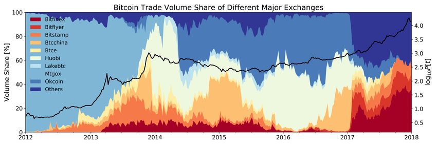
I.    Introduction
From an investment point of view, in the past decade, Bitcoin has become known for two main reasons:
its extraordinary return potential in phases of extreme price growth as well as regular massive crashes.
For instance, as a consequence of the most recent crash in mid-December 2017, a book-to-market value of
more than 200 Billion US Dollars of Bitcoin’s total market capitalization evaporated within only six weeks,
resulting in a cumulative loss from the peak of about two thirds in market value of the digital currency.
The massive crash was preceded by a no less impressive fiftyfold price boost over a time period of just two
years. Given the turbulent market history that Bitcoin has undergone since its inception in 2008 (Nakamoto,
2008), the recent bubble is not exceptional. In fact, as we will demonstrate in this paper, multiple overlapping
short- and long-term Bitcoin price bubbles have appeared between 2012 and 2018. It is our purpose here to
document this sequence of bubbles and crashes.
  At the time of writing, the combined capitalization of all existing cryptocurrencies still amounts to less than
one percent of the world GDP (Mossavar-Rahmani et al., 2018), a fact illustrating the still low significance
of this market in the global economic context. Nevertheless, cryptocurrencies, and especially Bitcoin as a
precursor of this new asset class, have drawn increased attention of the scientific and investment communities,
due to the strong growth of the sector over the past years as well as the technological and economic prospects
that are promised.
  There have already been a number of studies examining the statistical properties of Bitcoin returns. Pichl
and Kaizoji (2017) model the time-varying realized volatility of Bitcoin and found it to be significantly larger
compared to that of fiat currencies. Urquhart and Zhang (2018) study a variety of GARCH volatility models
and test the hedging capability of the crypto-coin against other currencies. The hedging properties against
other asset classes were investigated by Bouri et al. (2017). Bariviera (2017) provides evidence for volatility
clustering through a long memory Hurst exponent analysis. Furthermore, Osterrieder and Lorenz (2017)
find much larger magnitude in the heavy tail of the Bitcoin return distribution compared to conventional
currencies. Additionally, Begušić et al. (2018) determine even larger tail risk than usually seen in stocks.
Donier and Bouchaud (2015) investigate Bitcoin liquidity based on order book data and, from this, accurately
predict the size of price crashes. Other approaches to econometric Bitcoin modeling are outlined in Fantazzini
et al. (2016).
  Besides the purely statistical properties of the Bitcoin financial time series, there has been growing in-
terest in the social component shaping Bitcoin price dynamics, as well. Kristoufek (2013) firstly observed
a bidirectional relationship between web search queries and Bitcoin prices. Moreover, Garcia et al. (2014)
detect positive feedback loops between Bitcoin prices, user numbers of the Blockchain network and search
queries. They successfully implement a profitable Bitcoin trading strategy exploiting these social dynamics
(Garcia and Schweitzer, 2015). Likewise, Glaser et al. (2014) investigate the link between Bitcoin prices,
Blockchain network and search query data. They observe that “Bitcoin users are limited in their level of
professionalism and objectivity” because they primarily utilize Bitcoin as a speculative investment. An anal-
ysis of the Bitcoin user base in more depth is carried out by Kim et al. (2017) who apply topic modelling
to Bitcoin forum posts and test the predictive power of a deep learning model that is trained on the used
forum data. Further contributions to the characterization of the Bitcoin community are also summarized in
Fantazzini et al. (2016).
  These studies of the dynamics of Bitcoin’s price and of its associated social dynamics suggest that Bitcoin
buyers have been attracted by the sky-rocketing price performance of the cryptocurrency and have been
influenced by news and social media. This is typical of previous financial bubbles. Indeed, the media

                                                       2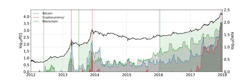
as well as many pundits have drawn parallels between the Bitcoin phenomenon and former extraordinary
financial bubbles such as the Tulip Mania or the Mississippi bubble. In the study presented below, we
provide confirming evidence and quantitative analyses that strongly support the conclusion that Bitcoin has
behaved as a highly speculative asset exhibiting strong bubble activity.
   In order to test for financial bubbles, we use the Log-Periodic Power Law Singularity (LPPLS) model.
First introduced as a calibration model by Sornette et al. (1995), it was elaborated into a rational expectation
bubble model in (Johansen et al., 1999, 2000) to provide real-time diagnostics of bubbles and forecasts of
crashes. A few studies have already applied the LPPLS model to analyse a few Bitcoin bubbles (see for
instance (Macdonell, 2014; Bianchetti et al., 2018a,b)). Here, we present a comprehensive general method-
ology to identify and classify the complete set of Bitcoin bubbles (over time scales larger than one month)
that occurred within the studied time period on the Bitcoin to US Dollar exchange rate series, both at short
and long time scales. The methodology for bubble characterization is completely automatized and can be
applied to any asset price time series, making it a robust measure for bubble detection.
  We identify three massive long bubbles and ten short bubbles. The temporal coexistence of these bubbles
underscores the multiscale nature of bubbles. It motivates the development of metrics that can be used to
separately identify evolving short and long bubble dynamics. We explore two techniques for this: (i) the
LPPLS Multi-Scale Confidence Indicator (Sornette et al., 2015; Zhang et al., 2016) and (ii) the characteri-
zation of bubble burst scenarios obtained by clustering the set of LPPLS calibrations over time scales and
predicted critical times. The forecast ability of the metrics to diagnose bubbles in real time and predict
crashes is evaluated. The present study complements and extends the one presented by Wheatley et al.
(2018), which focused on the identification of a proxy for the fundamental value of Bitcoin and a preliminary
assessment of predictability of a subset of the bubbles studied here. Here, we dwell much more in exploiting
the information contained in the LPPLS model calibration using the two mentioned sophisticated indicators.
  The paper is structured as follows. Section 2 describes firstly the generalised Epsilon Drawdown Method
that serves to identify the end times of long and short bubbles from January 2012 to February 2018 in the
Bitcoin price dynamics. The second part of the section explains how the Lagrange Regularisation Approach
provides an efficient determination of the beginning of the bubble regimes. The section concludes with a
summary of the main characteristics of the identified long and short bubbles. Section 3 analyses the main
socio-economic drivers behind the three long bubbles, and presents a series of useful metrics. Section 4
simulates a real-time assessment of the risks of the on-going bubbles. Section 5 concludes.

                            II.     Bitcoin Bubbles and Crashes
Before performing a predictive bubble analysis on Bitcoin, we need to construct a catalog of the bubbles
that actually occurred. Identifying a bubble ex-post would seem to be a straightforward job, but it is not.
A bubble could perhaps be defined as a large abnormal price increase, which then bursts in a crash. This
intuitive description is however quite naive, hard to conceptualize and full of traps, as it requires the implicit
definition of “abnormal price growth” and “crash”. In order to measure abnormal price increases, a reference
frame or process against which deviations can be gauged, must be defined, with the obvious criticism that,
when employing such a reference process, a bubble may be incorrectly diagnosed due to an untrue underlying
benchmark model, an issue that makes the diagnostic of a bubble a joint-hypothesis problem (Fama, 1991).
Moreover, a crash is also not easy to define, as it is a mixture of a large loss over some relatively short duration
that seems exceptional compared to the regular asset price movements. In the literature, we find a plethora

                                                         3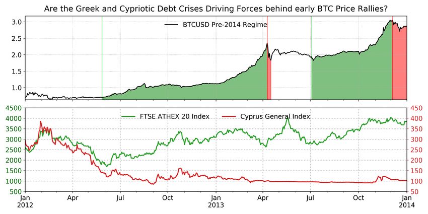
of different definitions, giving an overall impression of unpleasant arbitrariness. Thus, in this section, we
develop a methodology that combines several metrics to systematically and automatically identify the start
and end of long and short bubbles, the size and duration of the subsequent crashes, as well as quantitative
characteristics of the bubbles. The bubbles and following crashes, which are diagnosed in this way, will
provide the targets for our subsequent predictive analyses.

A.   Identification of the Peak Times of Long and Short Bubbles
Here, we present a straightforward method to identify the peaks of each bubble, where changing the value
of a single parameter allows us to scan bubbles of different durations. Our bubble diagnostic algorithm is
based on an extension of the Epsilon Drawdown Method developed by Johansen and Sornette (1998, 2001)
and further used in (Johansen and Sornette, 2010; Filimonov and Sornette, 2015). See Appendix A for the
detailed description.
  The key idea is to identify a bubble as a price run-up, the “drawup”, defined as a succession of positive
returns that may be interrupted by negative returns no larger in amplitude than some pre-specified tolerance
level ε. The bubble crash or correction phase corresponds to the subsequent “drawdown”, defined as a
succession of negative returns that may be interrupted by positive returns no larger in amplitude than
the pre-specified tolerance level ε. By construction, drawup and drawdown periods must be alternating
and directly following each other. In this way, a price trajectory can be systematically decomposed into a
sequence of alternating, consecutive price drawup and drawdown phases.
  The tolerance parameter ε is defined as the product of the realized volatility σ, estimated over a running
time window of duration w, and a constant, pre-set multiplier ε0 . The larger ε0 or σ, the bigger are the
oppositely directed price movements that are tolerated in a given developing drawup or drawdown. A drawup
(resp. drawdown) ends when a negative (resp. positive) (successive) return, whose amplitude exceeds ε, is
observed.
   In order to obtain robust results, we scan ε0 from 0.1 to 5 in steps of 0.1 and w from 10 to 60 days in
steps of 5 days, yielding 50 × 11 = 550 pairs (ε0 , w). For each pair, we run the Epsilon Drawdown Method
over the time series of the Bitcoin price expressed in US Dollars (btc/usd ) from Jan. 2012 to Jan. 2018, and
obtain a unique sequence of drawups and drawdowns. For each sequence, we record the peak times {tp },
defined as the end dates of all drawup periods that are contained in the sequence. Scanning over the 550
pairs (ε0 , w) gives us 550 sets of peak times {tp }. Next, for each daily date t in the observed time frame,
we count the number of times that this date was identified as a peak time over the whole set of 550 pairs
(ε0 , w). Dividing the resulting number by 550 gives us the fraction ft of pairs (ε0 , w) that have the date t
qualified as a drawup peak. We define large peaks, interpreted at the end of long bubbles, as those dates
such that ft > 0.95. We define intermediate sized peaks, interpreted at the end of short bubbles, as those
dates such that ft > 0.65. Intuitively, we therefore assume that large peaks are recognized in most of the
trials while small to intermediate peaks are identified fewer times.

                                                      4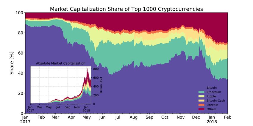
Epsilon-Method: Identified Peak Times of Potential Short Bubbles
                       1                           2 3          4     5 6            7       8    9 10
            4
            3
log10P(t)

            2
        1
        2012                2013           2014            2015            2016            2017          2018

Figure 1. Bitcoin Bubble Peaks identified by Application of the Generalized Epsilon Draw-
down Procedure between 2012 and 2018. Depicted in both panels is the logarithm of the Bitcoin to US
Dollar exchange rate (black line, grey region) from Jan. 2012 to Jan. 2018. The vertical red lines indicate
the bubble peaks that were identified according to the procedure outlined in the text. (Upper frame): the
three vertical lines indicate the peaks obtained with the condition ft > 0.95 (see text) and can be interpreted
as the peak times of long bubbles. (Lower frame): the 10 vertical lines indicate 10 peaks, other than the
three peaks of the upper frame, selected with the condition ft > 0.65. They can be interpreted as the peaks
of short bubbles.

     Figure 1 shows the results of the application of our procedure for the identification of bubble peak times
to the btc/usd log-price trajectory from Jan. 2012 to Jan. 2018. The upper frame shows three vertical lines
identifying the three peaks with the condition ft > 0.95. These three peak times are pleasantly coincident
with the ends of the three largest bubble regimes of the Bitcoin price in US Dollars from Jan. 2012 to Feb.
2018. The lower frame shows 10 vertical lines identifying the 10 peaks, other than the three previous peaks,
selected with the condition ft > 0.65. These 10 peak times will be interpreted below as the ends of shorter
bubble regimes. Note that these sets of peak times are robust with respect to reasonable changes of the
thresholds 0.95 and 0.65.

B.              Identification of the Beginning Times of Long and Short Bubbles
Following the above systematic determination of the main bubble peak times, we next need an automatic,
unbiased determination of the beginning times of the corresponding bubble regimes. For this, we use the
Log-Periodic Power Law Singularity (LPPLS) Model first introduced by Sornette et al. (1995) and elaborated
upon by Johansen et al. (1999, 2000), which combines a description of the faster-than-exponential transient
price acceleration with an increasing frequency of volatility fluctuations that are deemed characteristic of
a bubble regime. A summary of how the LPPLS model derives from the Johansen-Ledoit-Sornette model

                                                            5
(Johansen et al., 1999, 2000) is given in Appendix B. The LPPLS formula reads
LP P L(φ, t) := E[ln p(t)] = A + (tc − t)m B + C1 cos(ω ln(tc − t)) + C2 sin(ω ln(tc − t))
(1)
The model includes seven parameters φ = φ1 ∪ φ2 , of which four are linear φ1 = {A, B, C1 , C2 } and three
are nonlinear φ2 = {m, ω, tc }. The calibration methodology of the LPPLS model to a given price time series
is explained in Appendix C. In a nutshell, we apply a two-step procedure. For a fixed value of the triplet
(tc , m, ω), we solve analytically for the four linear parameters, which are solution of a linear matrix equation
deriving from the Ordinary Least Squares formulation. We perform a grid search in the (tc , m, ω)-domain,
followed by a nonlinear minimization, with the conditions that tc − t2 lies between 0 and t2 − t1 , 0 < m < 1
and 1 < ω < 50.
The fit of bt/usd log-price trajectory by the LPPLS formula requires the choice of a specific time window
[t1 , t2 ]. The end time t2 can be chosen at the bubble peak in post-mortem analyses. In order to diagnose
and eventually forecast the future price evolution, in an ex-ante predictive framework, t2 would represent
the “present time”, up to which the price history is available for analysis. Choosing the beginning time t1
(or equivalently the window size dt := t2 − t1 + 1) is less straightforward. Ideally, one would like to have t1
as the beginning of the current bubble or later if a bubble is developing, such that non-bubble phases, i.e.
phases of regular price growth, are excluded from the data to analyse.
To determine the beginning of a bubble, we implement the Lagrange regularisation Approach introduced
by Demos and Sornette (2017b). For a fixed t2 , we scan t1 from t2 − 29 to t2 − 719, corresponding to 691
windows ranging from 30 to 720 trading days. In principle, taking into account all LPPLS fits over the 691
time windows, the beginning of the bubble is defined as the time t∗1 that gives the “best” fit quality. Naively,
one could use the square root of the normalized sum of squared errors, also known as the root-mean-square
(rms), and choose t∗1 as the value that minimizes the rms. However, this procedure is incorrect as it does not
account for the fact that smaller windows will be favoured, due to their smaller number of degrees of freedom.
Demos and Sornette (2017b) observed that applying a simple correction to account for this bias, which is
linear in the window size (t2 − t1 ), behaves quite well and was efficient in a number of tests and real-life
case studies. This Lagrange Regularisation Approach is recalled in Appendix D. We apply the method to
the btc/usd rate in the same time frame as before. We impose the constraint that, for a given developing
bubble, its start time t∗1 cannot be earlier than the previous peak, as determined in Figure 1.
C. List and Main Characteristics of the Long and Short Bubbles
Combining subsection II.A which provides the set of bubble end times with subsection II.B for the deter-
mination of their beginning, we obtain a set of bubbles encoded by their time interval [t∗1 , tp ], i.e. the time
frame ranging from start to peak of the bubble. By definition, after the peak time of a bubble, a drawdown
starts, which initiates the crash or correction regime. We define the end of this correction regime as the
time at which the price reaches its minimum value over the time interval starting from the beginning of the
drawdown up to the start time of the next identified bubble. For the last analyzed bubble, we simply take
the price minimum between the bubble peak and the last available data point. The intermediate regime
separating the previous crash end and the next bubble start, if there exists one, is then defined as a phase
of normal price growth.
From the knowledge of start, peak and crash end dates of a bubble, as well as its price trajectory, we
calculate the bubble size in percent, defined as the cumulative return between bubble start and peak for
6Identified Long Bubbles and Crashes
1 2 3
4
3
log10P(t)
2
1
2012 2013 2014 2015 2016 2017 2018
Identified Short Bubbles and Crashes
1 2 5 6 7 8 9 10
4
3
log10P(t)
2
1
2012 2013 2014 2015 2016 2017 2018
Figure 2. Bitcoin Bubbles from January 2012 to February 2018. The three resulting identified
long (top panel) and eight short (bottom panel) bubbles, remaining after filtering the bubble characteristics.
The green bands delineate the bubble growth phases, while the red shaded regions represent the associated
crashes or correction regimes. The grey areas indicate phases of normal price growth, as defined in the text.
The numbers to the left of the vertical red lines map to those given in Figure 1.
each bubble. The bubble duration is computed as the number of days from bubble start to peak. The crash
size is calculated as the cumulative return between the peak time and crash end date.
Putting together the start, peak and crash end dates, the three peak times of the top frame of Figure 1 are
thus the end time of three “long” bubbles, for which we now have the systematically determined beginning
time and other characteristics, which are summarized in Table I.
For short bubbles to be determined among the 10 candidates associated with the peaks shown in the
lower panel of figure 1, we want to avoid very short spells and thus impose two additional filters: a “short”
bubble is such that it duration is at the minimum 30 days and its size larger than 25%, i.e. a short bubble
has its price increase by at least 25% over at least 30 days. For the set of ten short bubble peak times shown
in the bottom frame of Figure 1, we find that eight of them qualify as end times of short bubbles, whose
characteristics are also summarized in Table I. Two of the ten peaks (Peaks 3 and 4) are excluded as not
being preceded by a sufficiently large price increase (actually, they are local peaks within or just after a very
low drawdown shown in Figure 2(a)).
Figure 2 shows the three identified long (top panel) and eight short (bottom panel) bubbles. At a first
coarse-grained level of description, the top panel suggests that the Bitcoin history can be divided into three
main regimes: (i) a pre-2014 phase of intense price growth, (ii) a 2014-2016 long drawdown and side-way
regime, followed by (iii) the massive two-year long bubble that recently burst at the end of 2017. The bottom
panel shows that the two large-scale bubbles from 2012 to end of 2013 and from 2016 to end of 2017 are
themselves composed of shorter bubbles, some of them still with impressive amplitudes. We now turn to
7describe them briefly from a socio-economic point of view.
Long Bubble Data
Nr. Bubble Start t∗1 Bubble Peak tpeak Crash End Date Duration [days] Bubble Size [%] Crash Size [%]
1 2012-05-28 2013-04-09 2013-04-16 316 4416 -70.27 NA
2 2013-07-03 2013-12-04 2015-01-14 154 1367 -84.83 NA
3 2016-01-15 2017-12-18 2017-12-25 703 5152 -26.55 NA
Short Bubble Data
Nr. Bubble Start t∗1 Bubble Peak tpeak Crash End Date Duration [days] Bubble Size [%] Crash Size [%]
1 2012-05-07 2012-08-16 2012-08-20 101 165 -25.11 Y
2 2014-04-15 2014-06-03 2014-06-25 49 28 -16.38 Y
3 2014-06-30 2014-10-14 2014-10-23 106 -37 -11.45 N
4 2014-10-23 2015-03-11 2015-04-13 139 -16 -24.75 N
5 2015-04-13 2015-07-27 2015-08-24 105 31 -28.74 Y
6 2015-08-26 2015-11-04 2015-11-11 70 80 -24.04 Y
7 2016-01-15 2016-06-16 2016-08-02 153 112 -29.56 Y
8 2016-08-03 2017-01-04 2017-01-11 154 97 -30.16 Y
9 2017-03-24 2017-06-06 2017-06-07 74 210 -6.86 Y
10 2017-06-07 2017-09-01 2017-09-14 86 83 -34.42 Y
Table I. Basic Information about all Qualified Bubbles. Dates and characteristics defining each
bubble cycle. The last column indicates whether a potential bubble peak passed the bubble conditions
defined in the main text.
III. Socioeconomic Drivers behind Bitcoin Bubble Dynamics
Having characterized the main bubble events, it is useful to put them into context and expose their key
drivers, as well as the developments and events that promoted their nucleation or caused their sudden
crashes. In particular, we analyze the possible causes of the nucleation and main drivers for the growth of
the three major identified Bitcoin long bubbles that occurred between 2012 and 2018. The history of Bitcoin
at its early stage was highly influenced by fiscal and monetary measures undertaken during the Eurozone
crisis. Later on, the development of the cryptocurrency was to a great extent influenced by increasing
demand from China, which evolved as a result of the emergence of major Chinese Bitcoin exchanges opening
up the markets for investors. Although it had a strong temporary impact on Bitcoin in the short term, the
shutdown of Chinese exchanges that occurred in early 2017 caused no persistent loss in its capitalization.
Quite the contrary, the year of 2017 is characterized by remarkable growth dynamics due to the contagion
of the Bitcoin bubble to a general cryptocurrency bubble. Finally, at the end of 2017, the most recent long
bubble crashed with a shocking intensity, removing 60% (up to Feb. 2018) of the cryptocurrency market
capitalization measured from its peak in Dec. 2018. The following sections examine this history in more
details.
A. First Long Bubble: May 2012 - April 2013
The financial crisis of 2007-2008 put economies worldwide into a fragile state. It also helped reveal the
unsustainable debt level and the longstanding financial mismanagement of some small and medium sized
economies within the European Union such as Greece, Ireland, Portugal, Spain, Iceland and Cyprus. In
particular, the crises in Cyprus and Greece stand out by their intensity and consequences. Notice that both
countries reached their worst economic state for decades in 2012, as demonstrated in the bottom panel of
8Figure 3. The economic decline was accompanied by ongoing discussions about further bailout programs for
Greece, as well as requests of the Cypriot government for a bailout of its financial sector which the country’s
economic well-being largely relied on (Wilson et al., 2012).
The emerging mentality of distrust in governments and financial institutions triggered a wave of bank runs
and hunts for monetary safe havens. Bitcoin, proposed as an alternative store of value that was primarily
intended to be uncontrollable by governments and independent of monetary policies (Nakamoto, 2008),
appeared to ideally meet these requirements. It is no coincidence that the nucleation of the first Bitcoin long
bubble occurred at the exact time when the Greece and Cypriot indices reached their troughs.
Figure 3. Comparison of the Evolution of Bitcoin Price and Greece as well as Cypriot Financial
Market Indices. The top panel shows the Bitcoin log-price trajectory from Jan. 2012 to Jan. 2014. In
the bottom panel, the Greek ATHEX 20 Index (left scale), as well as the Cyprus General Index (right scale)
are depicted over the same period. The financial market indices of Spain, Portugal and Ireland follow paths
highly correlated with that of the Greece index, as their indices bottomed out during approximately the
same time. [Data Source: Datastream (2018)]
On March 16, 2013, a critical point was reached for the Cypriot economy, when a bail-in tax that largely
affected the deposits of account holders at Cypriot banks was declared. The announcement created a massive
wave of bank runs triggered by account holders trying to protect their personal savings (Thompson, 2013).
This coincided with the last accelerating growth of Bitcoin’s price, before its crash in April 2013 (Farrell,
2013).
The described developments in Cyprus were anxiously observed in other Eurozone countries, for instance
in Spain, where people feared that similar governmental interventions could lead to the loss of their own
savings (Warner, 2013). Serving as a store of value that could not be seized by any institution, Bitcoin
arrived on the scene, perceived as the perfect alternative investment. Figure 4 illustrates the consequential
flow towards the cryptocurrency in form of soaring Blockchain transactions around the time of the bubble
nucleation of Long Bubble 1. As a response to the increasing demand, in the course of bubble growth, the
price of a Bitcoin was catapulted up by an incredible 4400% above the price mark of 100 USD per Bitcoin.
9Figure 4. Evolution of the Number of Transactions on the Blockchain Network. The grey
shaded region delineates the logarithmic number of Bitcoin Blockchain transactions (right scale). In 2012, a
jump of the transaction number occurred in response to the large demand surge by investors seeking Bitcoin
as a safe haven. [Data Source: Blockchain.info (2018)]
The bubble reached maturity in early April 2013. Specifically, after peaking on April 9th , it burst, with
approximately 70% of Bitcoin’s market capitalization disappearing within one week. The actual cause of
the crash was a reaction to instability announcements on MtGox, the by then worldwide biggest Bitcoin
Exchange in terms of Bitcoin exchange-traded volume, which was suffering the consequences of a hacker
attack (Buterin, 2013).
Obviously, the event leading to the crash was not directly related to the political backgrounds of the
Eurozone and Cypriot Crises that actually initiated the bubble. As is often the case in the bursting of a
bubble, one should distinguish the proximate cause of the crash, which is in general unrelated to the source
of the bubble, from the fundamental origin of the crash, which is that the Bitcoin market had progressively
evolved towards a fragile, unstable, critical state, associated with a large susceptibility to adverse news.
B. Second Long Bubble: July 2013 - December 2013
The second long bubble matured at the end of 2013 after an approximate thirteen-fold increase from its
post-crash recovery level after the first long bubble. As the European debt crisis was still well underway
during this time, again, the attraction to the alternative decentralized Bitcoin contributed to its price surge.
But, one should not underestimate a number of additional factors that contributed to the emergence of this
bubble: the adoption of Bitcoin in China, the FBI shutdown of the Darknet drug market Silk Road, as well
as the growth and increasing technical sophistication of the Bitcoin mining community.
Figure 5 presents the history of the birth and trading volumes of the main Bitcoin exchanges from 2012
onward. The blue inset plots show the births and absolute volumes handled by the different exchanges.
The light grey area shows the logarithmic summed transaction volume of all of these exchanges that are
still active today, while the dark area sums the volume of all listed exchanges. It can be seen that major
Chinese exchanges were founded in the nucleation phase of the second long bubble, amongst them Huobi
and OKCoin, which later on became the dominating Bitcoin exchanges in China (Bovaird, 2016).
10Bitcoin Exchange-Traded Volume over Time, Aggregate and per Exchange. 8
log10Volume
4
3 7
2 Bitflyer
log10P[t]
Lakebtc
1 Huobi
Okcoin
Bitfinex
0 Btce
Bitstamp
Btcchina
Others
Mtgox
2012 2013 2014 2015 2016 2017 2018
Figure 5. The Evolution of Bitcoin Exchanges in Terms of Trading Volume. The dark grey area
(right scale) represents the total log-volume of all analyzed exchanges. The light area shows the volume of
only the exchanges that are still in business as of end 2018. The blue inset plots schematically show the
evolution of traded log-volume of the single exchanges that are listed next to the right plot axis. Note that
the inset plots are ordered according to the dates of entry into service of the different exchanges. Hence, from
these plots, the temporal origination of exchanges can be compared. [Data Source: Bitcoinity.org (2018)]
The emergence of new Bitcoin exchanges significantly facilitated market entrance for the numerous pri-
marily China-based investors to the Bitcoin market. Ultimately, the wave of new investments drove prices
above the 1000 USD level for the first time. Figure 6 shows that the share in total traded volume of Chi-
nese exchanges started to really break through during the second long bubble, in the phase of most intense
growth. Before that, MtGox held the majority of the market share. However, its market share plummeted
from more than 50% at the beginning of the bubble down to a mere 10% at its peak. The corresponding
lost fraction had been replaced by trading volume on the uprising Chinese exchanges.
As the bubble was developing at fast pace, on October 2nd , 2013, the online drug market Silk Road, which
enabled customers to buy illegal substances anonymously, was shut down by the FBI and its alleged founder
imprisoned (Pagliery, 2013). This signaled to the Bitcoin community that the legal authorities had their eye
on the cryptocurrency and intended to prevent any illegal activities related to it by all means. Although Silk
Road was the first, but not the only darknet drug market, its seizure had wide implications and hit the news
headlines heavily. The closure of Silk Road symbolically set free Bitcoin as a proper investment for more
cautious investors who, until then, were deterred by its illegal usage as drug money. The subsequent build-up
of a clean image for Bitcoin was also recognized by the US senate, which as a consequence announced an
official hearing about the utility and future prospects of the digital currency (US Senate, 2015). The event
is seen as a further beneficial factor contributing to the immense price surge seen in the second long bubble
(Wile, 2013).
11Figure 6. Volume Share of the Top Ten Bitcoin Exchanges. Shown on the left scale is the percentage
share of the Bitcoin volume traded on each exchange with respect to total traded volume. Notice the surge
of the two main Chinese exchanges, OKcoin and Huobi towards the end of the second long bubble, as well
as the constant decrease of the market share of until then dominating Japan-based exchange MtGox. [Data
Source: Bitcoinity.org (2018)]
Figure 7 hints at the third contributing factor for the price growth during the bubble. The logarithmic
hash rate power of the miners computing transaction blocks on the Blockchain is shown, as well as the
logarithmic number of registered wallets. Notice that the hash rate grew at a much faster rate compared to
the number of wallets over the period starting with the first long bubble. The highest rate of increase was
reached during the second half of 2013, coinciding with the second long bubble.
The number of registered wallets is a measure for the size of the network of users operating directly on
the Blockchain. Hence, the hash rate increasing faster than the user base signals that on average miners
enhanced their individual mining power during the period. This was most likely achieved through the usage
of more efficient technical mining hardware. We conclude that, in addition to Bitcoin adoption effects in
China and the image improvement of Bitcoin, we can see the effect of the ramp-up behavior of hash power
as an indication of increased mining sophistication.
Concerning the improvement in hardware and mining technology, we note that the first long bubble played
an important role as a precursor to the second one. As the Bitcoin price increased for the first time to a fairly
high level, miners were incentivized to invest in mining hardware. At the relatively high price of a Bitcoin
compared to the computational effort required to create it, it was profitable for them to enter the mining
business. The increasing number of miners itself then triggered a feedback mechanism. It can be seen as a
self-fulfilling, self-reinforcing bubble in the following sense: the larger the price, the larger the incentive to
invest in hardware computing power; the more mining there is, the more activity there is on the blockchain
that attracts more and more users and buyers, the more the price increases. But, the faster growing variable
should quickly become the hashing difficulty. The loop is closed when the incentive of miners to invest in
hardware rises again.
12Figure 7. Growth of Bitcoin Blockchain Network User Base and Increase in Mining Power.
Superimposed to the Bitcoin price in log-scale (left axis), the total hash rate and the number of registered
wallets are shown (right axis). The largest rate of increase of the total hash rate can be observed over the
course of the second long term bubble in 2013, a fact signalling an increasing level of miners’ technique
sophistication. A second, more subtle acceleration of the hash rate can be seen around the nucleation of the
third long bubble. [Data Source: Blockchain.info (2018)]
There are two major triggers for the crash that started in Dec. 2013 and was followed by a long drawdown.
Firstly, the Chinese Government suddenly prohibited financial institutions from using Bitcoin when the
price of a Bitcoin was close to the peak of the bubble in December 2013 (Hill, 2013). The announcement
destabilized the currency and sent it into free fall. Secondly, during February 2014, when there was still
hope for the price to recover, MtGox suspended trading (see Fig.6) and filed for bankruptcy protection from
creditors after a major account robbery of at least 700,000 missing or stolen Bitcoins of customers had been
reported (Zuegel, 2014).
The demise of MtGox was perceived as a major setback for the Bitcoin world. Account holders of the
exchange lost money that was not or hardly recoverable due to the difficulty of tracing it. Once more, this
led to a huge loss of Bitcoin’s trustworthiness, which already had been questioned over and over again in the
past. These adverse circumstances set the currency off into a one-year long decline.
C. Third Long Bubble: January 2016 - December 2017
The winners of the long Bitcoin price drawdown that took place from 2014 until mid-2015 were clearly the
China-based Bitcoin exchanges. At the time of the closure of MtGox, they had already occupied the majority
(more than 90%) of all exchange-traded volume, as can be seen by looking back at Figure 6. Within the three
years following 2014, Bitcoin volume formation on Chinese exchanges contributed to roughly an hundredfold
increase in global volume (see Fig.5). It is this rising demand for Bitcoin from Chinese markets originating
during that time, which can be seen as a major precipitating factor for the nucleation of the third long term
bubble, whose start we identify around the beginning of 2016. This leaves open the question where this
increased demand originated from? We identify the devaluation of the Chinese Yuan as a main promoting
factor for the rising interest in cryptocurrencies in China and thereby the formation of the third long bubble.
13Figure 8. Development of Bitcoin in Parallel to the Chinese Yuan. The Bitcoin log-price (top
panel) and the Chinese Yuan vs. US Dollar (CNY/USD) exchange rate (bottom panel, left axis). A change
of regime occurred in the Chinese currency simultaneously to the decline of Chinese exchange-traded Bitcoin
volume (bottom panel, right axis) at the beginning of 2017. [Data Source: Datastream (2018)]
Figure 8 shows a change of regime in the exchange rate of the Chinese Yuan (CNY) versus the US Dollar
from 2014 onward. In August 2015, the depreciation of the Yuan was enforced through a devaluation of the
currency by the People’s Bank of China, PBoC, as seen by the sudden jump in the rate. This devaluation
was motivated by the desire to raise the competitiveness of exporting firms. From there on, a continuous
weakening of the Renminbi developed until January 2017.
As a reaction to the depreciation of their currency from 2014 onward, Chinese market participants tried to
transfer their money to what they perceived as safer stores of value, causing an outflow of capital from China
(Gautham, 2016). As for the average Chinese investor, limitations in terms of foreign-exchange investments
were quite restrictive, Bitcoin was a straightforward solution to store value (Suberg, 2016). As a response to
the devaluation of the Renminbi, one can observe indeed a large increase in demand for Bitcoin in form of
rising trading volume and growing prices from mid 2015 onwards. Note specifically the period of devaluation
of the Chinese Yuan (during the last quarter of 2015) preceding the start of the third long bubble.
In January 2017, the Central Bank of China instructed the - until then widely unregulated - Chinese
Bitcoin exchanges to comply with the country’s financial regulations (Rizzo, 2017), as it suspected illicit
exchange activities such as money laundering, as well as volume manipulation (through wash trading) that
was made possible by the zero trading fee policy of exchanges (Olszewicz, 2017). In a first intervention, the
biggest Chinese Bitcoin exchanges BTCC, Huobi and OKCoin (Higgins, 2017) were forced to reintroduce a
non-zero trading fee structure and to stop leveraged trading (Bovaird, 2017). The measure led to the huge
slump in exchange trading volume that can be observed in Figure 5. Simultaneously, the Short Bubble 8
(see Figure 2 and Table I) burst in a 30% crash.
Chinese exchanges started with their zero trading fee policy in late 2013. It has been estimated that, due
14to the ongoing manipulations of trading volume, the volume reported by exchanges had been overstated by
up to forty times the true volume (Woo, 2017). Hence, the crash in trading volume partly seems to represent
a normalization to realistic levels (Wong, 2017), as with the introduction of trading fees, volume could not
be generated at no cost, any longer.
In a further regulatory move, in February 2017, the PBoC again exerted pressure on Chinese exchanges
causing them to halt Bitcoin withdrawals (Goh, 2017), while still tolerating withdrawals executed in the
domestic currency Yuan (Solana, 2017). Effectively, this measure was intended to cut off the outflow of
Chinese money through Bitcoin.
In June 2017, the temporary withdrawal pause was ended, as exchanges had partly adapted to the
regulatory standards demanded by the PBoC (Arnold and Chen, 2017). These news implied an overall
positive outlook for Bitcoin’s future in China, promoting further rise in the price of the digital coin. In
September 2017, unexpectedly, Chinese regulators banned the so-called Initial Coin Offerings (ICOs) (Chen
and Lee, 2017), a novel procedure for the emission of new digital coins, emulating the Initial Public Offerings
of regular firms. Finally, in mid September, the Central Bank ordered Chinese exchanges to shut down all
trading activities on the Chinese market (Huang, 2017). This quick series of unanticipated events officially
put an end to cryptocurrency exchange business in China. The gradual decrease in trading volume and
closure of exchanges during 2017 is shown again in Figure 5.
Although in late 2017, cryptocurrency trading was proclaimed “Officially Dead In China” (Rapoza, 2017),
the actions undertaken by China’s Central Bank led to (i) a shift of exchange-based trading to OTC trading,
running on so-called peer-to-peer exchanges (Barclay, 2017), the most known of which was LocalBitcoins,
and (ii) Chinese exchanges such as Huobi and OKCoin moving their business abroad (Zhao, 2017). In this
way, although PBoC managed to prevent Yuan-based trading, the still present large if not increased demand
was eventually just redirected to other markets (Redman, 2017). Thus, the imposed regulatory constraints
did not have any permanent influence on the global evolution of the price of Bitcoin. This is also backed by
the fact that, throughout 2017, the Bitcoin price recovered fast from drawdowns resulting from China-related
negative news.
Besides the large contribution of Chinese-based Bitcoin investing to the formation of the third long bubble,
there were other factors driving the growth of the bubble. The third long bubble was punctuated by a number
of short bubbles that burst abruptly, but were followed by a fast recovery of the Bitcoin price, as seen in
Figure 2. There are several reasons for this behavior.
Going back to the nucleation of the third bubble in early 2016, as in the case of the second long bubble,
one witnesses an increase in the growth rate of the hash rate, with the total hash power then exceeding 1
ExaHash/second (= 1018 H/s !). Moreover, during 2016, several of the nowadays dominating BTC mining
pools became active (viabtc, btc.com, btc.top) (ViaBTC, 2018; BTC.com, 2018; BTC.TOP, 2018). This
development produced additional publicity for Bitcoin and pushed mining efficiency for individuals once
more. The fact that mining gains of pools are proportionally shared amongst miners according to their
power contribution provided a large incentive especially for weak miners to resume their mining activity, as
their chance of being rewarded for mining (within their lifetime) suddenly was ensured. The growth of the
mining network and associated hash power is a factor that may well have contributed to higher resilience
and fast recovery of the Bitcoin price during the massive, third long bubble.
15Figure 9. Google Trends Search Queries related to Bitcoin. The three grey shaded areas depict
the development of search requests for the terms Bitcoin, Cryptocurrency and Blockchain. For studies
demonstrating the relationship between such search queries and the Bitcoin price trajectory, we refer the
reader to (Kristoufek, 2013; Garcia et al., 2014). [Data Source: Google Trends (2018)]
The most distinct feature driving the acceleration of the Bitcoin price after the China exchange shutdown
was the growth of the cryptocurrency market as a whole. Figure 9 demonstrates that, besides skyrocketing
Google search queries for the term Bitcoin, from 2017 onward, a sharp increase in search queries for the term
Cryptocurrency occurred. Already from 2015 onward, rising requests for the term Blockchain can be seen.
This signals interest in Blockchain technology on its own that has been growing over the years, as well as
strongly enhanced interest in alternatives to Bitcoin from 2017 onward.
As a response to investor’s growing demand for alternative investments in the cryptocurrency market, the
emergence of a multitude of new digital coins ensued. Throughout 2017, the cryptocurrency market changed
its structure from being dominated by Bitcoin to a more diversified market offering numerous technologies
and variants of cryptocurrencies (Wu et al., 2018).
Figure 10 shows the dominance of Bitcoin at the beginning of 2017 over the complete cryptocurrency
market with its market share, measured with respect to the total market capitalization of the top 1000
cryptocurrencies, being as high as 90%. Within three months after February 2017, its relative market share
dropped by 50%, while its total capitalization value and that of other crypto-currencies continued to grow
at accelerating pace until Dec. 2017.
During the last two months of 2017, the overall capitalization of the crypto-market multiplied by a factor
four. As the idiom claims, “the rising tide lifts all boats”, and thus, the large inflow of fresh money to
the cryptocurrency market impacted most of the Altcoins as well as the still dominating Bitcoin. However,
with the crash following Dec. 18th , 2017, the value of Bitcoin and that of many cryptocurrencies has been
dropping, with Bitcoin losing sixty percent of its total value (as of February 2018), putting the Bitcoin
market share to an all-time low.
16Figure 10. Progressive Maturation of the Cryptocurrency Market during the Year of 2017.
Shown is the market share of the five largest capitalized cryptocurrencies Bitcoin, Ethereum, Ripple, Bitcoin
Cash and Litecoin, as well as the aggregate capitalization of the top thousand cryptocurrencies excluding
the five largest ones in the the year 2017 (shown as “Others”). Similarly, the inset plot depicts the evolution
of the absolute market capitalization. We can see that, within one year, Bitcoin lost a majority of its share
in the total market capitalization. This signals its possibly decreasing significance and, at the same time,
the growing number of competitive cryptocurrencies in the market. [Data Source: CoinMarketCap (2018)]
One can say that 2017 was the year of the cryptocurrencies. New competitors were constantly pushing
their coins as well as new tokens into the market. These coins and tokens were associated with new proposed
ideas of the application of Blockchain technology. As the market is becoming ever more complex every day,
the possibility for the release of a new coin making Bitcoin obsolete is perceived more likely. In contrast,
others note that Bitcoin may survive as a kind of relatively scarce digital “commodity” or asset, used by
investors as a storage of value and diversification vehicle.
We now turn to a more quantitative analysis of the various bubbles from 2012 to 2017 to recount how well
these bubbles (could) have been diagnosed in real time with metrics derived from the Log-Periodic Power
Law Singularity Model presented above in section II.B.
IV. Real-Time Bubble Identification
A. LPPLS Multiscale Confidence Indicators as Bubble Diagnostics
Following the methodology of Sornette et al. (2015) and Zhang et al. (2016), we use the LPPLS Confidence
Indicator as a diagnostic tool for the recognition of bubbles. In a nutshell, the LPPLS Confidence Indicator
at a given time t2 is the fraction of windows [t1 , t2 ], obtained by scanning t2 − t1 over a certain window size
interval, for which the calibration of the log-price of Bitcoin by the LPPLS formula (1) passes the criteria
shown in Table II. A large LPPLS Confidence Indicator value indicates that the LPPLS patterns with model
parameters passing the filtering conditions are found in a large fraction of time scales at this particular
17time t2 . This is then translated into a bubble diagnostic analysis, based on the hypothesis that the LPPLS
pattern is a characteristic feature of bubbles.
Parameter Filter Bounds Description Pre-Condition
Power Law Amplitude B (−∞, 0) - -
Power Law Exponent m (0, 1) - -
Log-periodic Frequency ω [4, 25] - -
Critical Time tc (0, dti ) - -
m|B|
Damping D [0.5, ∞) D= ω|C| -
ω tc −t1
Number of Oscillations O [2.5, ∞) O= 2π ln tc −t2 if |C/B| ≥ 0.05
Table II. Filter Conditions for Qualified LPPLS Fits. The table gives the parameter bounds that
were used to filter for qualified LPPL fits. The constraint on B ensures the existence of a positive bubble.
For m and tc , the boundaries are excluded to avoid singular behaviors in the search algorithm. The damping
factor quantifies the allowed downwards movements of bubble fits. The O-parameter measures the number
of oscillations that occur within the fit window [t1 , t2 ]. The filter on O is applied only when the amplitude
of the oscillations, as quantified by C, is sufficiently large relative to the power law amplitude B.
In order to capture the main relevant time scales of investment horizons, we propose to partition the
window sizes dt := t2 − t1 + 1 over which the LPPLS Confidence Indicator is calculated into three classes:
dt ∈ [30, 120] (short time scale), dt ∈ [100, 240] (medium time scale) and dt ∈ [200, 720] (long time scale).
The short time scale goes approximately from one month to five months. The medium time scale ranges from
6 months to a year (when there are approximately 250 trading days in a calendar year). The large time scale
goes from 10 months to approximately 3 years. Thus, for each t2 , we construct three LPPLS Confidence
Indicators, one for each set of window sizes. There are respectively 91, 141 and 521 differently sized windows
for the short, intermediate and long time scales. We refer to the ensemble of the three indicators calculated
in this way as LPPL Multiscale Confidence Indicators.
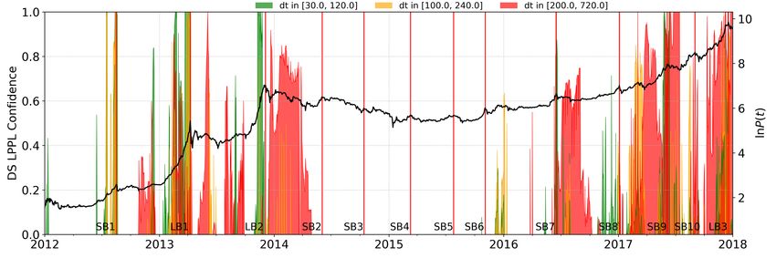
Figure 11. Diagnosing Bubbles over Multiple Scales using the LPPLS Confidence Indicator.
The LPPLS Confidence Indicator diagnoses bubbles nucleating over short (green), intermediate (yellow) and
long time scales (red). The larger the value of the metric at a given point in time, the larger the portion
of qualified LPPLS fits, indicating stronger bubble activity. The peaks of the bubbles, as documented in
Figure 2 and Table I, are depicted in red vertical lines.
Figure 11 depicts the LPPLS Multiscale Confidence Indicators, as described above, constructed on the
Bitcoin/USD price. One can observe that the short and intermediate indicators peak at or close to the
18corresponding bubble tops, providing useful diagnostics, in particular for the first three pre-2014 bubbles.
For the shortest bubble episodes such as Short Bubbles 5 and 6, there are no signals. This can be understood
from the choice of time scale: even the short time scale dt ∈ [30, 120] is too long, compared with the duration
of these two bubbles. This shows the importance of having a suitable set of indicators scanning the time
scales of interest. Although not all of the minor short bubbles are identified due to the mentioned limitation
of time scales, in all cases for which the LPPLS Confidence Indicator reaches its maximum value 1, a crash
follows.
After 2016, the LPPLS Confidence Indicator at the long time scale exhibits an increasing amplitude,
associated with the development of the third long bubble. Close to the peak in December 2017, the large-
scale LPPLS Confidence Indicator is close to its maximum level, providing a warning for an imminent massive
crash, following bubble price dynamics that evolved over the long term. Since the end of 2016, we have been
implementing this and other indicators to watch the development of asset price bubbles, amongst them the
many bubbles in the Bitcoin price: for instance, in our monthly report of the Financial Crisis Observatory on
the 1st December 2017, we pointed out the alarm generated in advance to the burst of the third long bubble
(see 1st December 2017 Synthesis report at www.er.ethz.ch/financial-crisis-observatory.html).
Overall, the LPPLS Multiscale Confidence Indicators over the three monitored scales provide a valuable
risk management metric for early recognition of emerging bubbles at short and long time scales as well as
their approaching bursts. In particular, the long bubbles are clearly identified in advance by the fact that
the three LPPLS Confidence Indicators peaked jointly for these long bubbles. The other non-synchronized
indicator peaks testify of the multiscale nature of bubbles in Bitcoin.
B. Predictions of Bubble Burst Times Using Ensemble Forecasting
B.1. Methodology
We now present systematic mock-up forecasts of the burst times of the three long and eight short bubbles
identified in Figure 2 and Table I. For each bubble, we position the mock-up “present” time of analysis t2
ten business days prior to the corresponding identified bubble peak date given in Table I. Next, for each
analysis time t2 , we identify the associated bubble start time t∗1 by means of the Lagrange Regularisation
Methodology, as explained in section II.A.
Based on the complete “frame” of each bubble [t∗1 , t2 ], we perform LPPLS calibrations over all windows
by scanning t1 from t∗1 to t2 − 29. Out of these t2 − t∗1 − 28 LPPLS fits, we again only keep those that pass
the filter conditions listed in Table II. For a given t2 , each of the remaining qualified fits is then characterized
by (i) its window size dt := t2 − t1 + 1 corresponding to the observed time scale and (ii) a forecasted horizon
tc − t2 , which is the estimated remaining time from the present time t2 up to the predicted end tc of the
bubble.
Because analyses performed over different window sizes may result in different forecasts, corresponding to
multiple price dynamics, we use the k-mean clustering method to identify clusters in the (dt, tc − t2 ) space
whose components yield common predictions for the critical time tc . Then, if a unique, well-defined cluster is
identified, this can be interpreted as a consensus forecast obtained over all the time windows included in the
cluster. If there are two well-defined clusters, similarly, one should conclude that the analysis suggests two
different scenarios for the future development of the bubble, and so on. We augment the k-mean clustering
method by using the Silhouette metric to determine the optimal number k̂ of clusters and thus of forecasted
scenarios. The details of the k-mean clustering implementation and application of the Silhouette metric are
19given in Appendix E.
Long Bubble Data
Nr. Analysis Date t2 Qualified Fits [%] Clusters k̂ Silhouette s̄k̂
1 2013-03-28 43 2 0.85
2 2013-11-22 40 2 0.84
3 2017-12-06 68 9 0.67
Short Bubble Data
Nr. Analysis Date t2 Qualified Fits [%] Clusters k̂ Silhouette s̄k̂
1 2012-08-06 59 2 0.58
2 2014-05-22 0 - -
3 2014-10-02 0 - -
4 2015-02-27 0 - -
5 2015-07-15 0 - -
6 2015-10-23 0 - -
7 2016-06-06 12 2 0.91
8 2016-12-23 33 3 0.75
9 2017-05-25 93 2 0.57
10 2017-08-22 0 - -
Table III. Summary of Cluster Data for Long and Short Bubbles. The first column enumerates the
three long bubbles and the ten additional peaks, which include the eight short bubbles, as qualified by the
method of Section II.A. The second column gives the “present” time t2 that was chosen ten business days
prior to the peak of each bubble. The third column gives the percentage of fits that are qualified. The fourth
column gives the optimal number of clusters. Finally, the fifth column lists the values of the Silhouette
coefficient corresponding to the optimal cluster configuration. For further information on the details of the
calculation, see Appendix E.
B.2. Long Bubbles
Table III shows that, for the long bubbles, between 40 and 68 percent of the fits are qualified according to the
filtering constraints from Table II. For the first and second long bubbles, two main scenarios are identified
while for the third longest bubble, we find up to nine scenarios, most of them being far to the future and
with few elements, thus unreliable and discarded. Figure 12 contains three panels, one for each of the three
long bubbles. Each panel shows the log-price of Bitcoin over the time interval of the full development of
the bubble together with, for each of the identified clusters, the 15 LPPLS fits (when they exist) having the
lowest sum of squared errors (SSE).
The top-left panel shows the first long bubble that peaked on April 9, 2013. The scenario corresponding
to the first largest cluster predicts the mean of tc to be 14 days in the future (after t2 ) with a standard
deviation of 9 days. The second, smaller cluster predicts tc to be 262 days in the future with a standard
deviation of 34 days. Hence, the first scenario is essentially telling us that the bubble peak is imminent, with
a quite precise bracketing of the true peak. Interpreting the fraction of fits belonging to this cluster as a
proxy for the probability for this scenario, we can attribute a probability of 80% (101 fits) for this scenario.
The second less probable (20% probability, 25 fits) scenario considers as possible that the bubble may
continue much longer, up to another year, before bursting. Given the interplay between the endogenous
herding dynamics captured by these scenarios and the exogenous shocks that continuously punctuated the
bubble development, in retrospect, these two scenarios appear reasonable possibilities when placing oneself
at the time t2 of the analysis. In hindsight, the highest probability scenario was the one that unfolded.
Turning to the second long bubble that peaked on December 4, 2013 and is shown in the top-right panel
20You can also read