Distinguishing different radioactive sources with operative plastic scintillators - Jyväskylän yliopisto
←
→
Page content transcription
If your browser does not render page correctly, please read the page content below
Distinguishing different
radioactive sources with
operative plastic scintillators

Master’s Thesis, 23.5.2018

Author:
Olli Virkki

Supervisors:
Kari Peräjärvi
Finnish Radiation and Nuclear Safety Authority, STUK
Ari Jokinen
Department of Physics, University of Jyväskylä
2
3

Abstract

Virkki, Olli
Distinguishing different radioactive sources with operative plastic scintillators
Master’s Thesis
Department of Physics, University of Jyväskylä, 2018, 80 pages

Plastic scintillators (PS) are widely used as radiation monitors in industry and bor-
der control. Besides being a fast scintillation material, the low material cost, efficient
bulk production and high sensitivity due to big sizes have made PSs a foundation of
most radiation monitors as they are fast and cheap to deploy and efficient detectors.
Due to their limited capabilities to distinguish different radiation sources, in the
past they were mainly used as rough counters only to detect radiation. The increas-
ing demand for different radioactive materials in industry and medical field increase
the risk of illicit and inadvertent use or radiation sources. As a counterpart, the
abundant naturally occurring radioactive materials (NORMs) in most cases do not
require further investigation. Minimizing unnecessary workload while keeping the
radiation monitoring efficient gives rise to the need of radiation source identification
methods.
The goal of this Master’s thesis is to offer insight for plastic scintillators from an
operational viewpoint. Possible next-generation operation modes for more precise
radiation monitoring as well as different characterization methods to probe the func-
tionality of a plastic scintillator are presented and tested in practice. The methods
can be executed in on-field conditions and are applicable for plastic and other scin-
tillation materials used in both operational and laboratory purposes.

Keywords: Plastic scintillator, Radiation monitoring, Scintillator characterization
4
5

Tiivistelmä

Virkki, Olli
Säteilylähteiden tunnistaminen operatiivisilla tuikeilmaisimilla
Pro-gradu tutkielma
Fysiikan laitos, Jyväskylän Yliopisto, 2018, 80 sivua

Muovisia tuikeilmaisimia käytetään laajasti säteilyvalvonnassa sekä teollisuudessa
että rajavalvonnassa. Niiden suhteellisen matalat materiaalikustannukset, massatuo-
tantokyky, tuikemateriaalin nopeus sekä suuret koot mahdollistavat nopean käyt-
töönoton ja korkeat havaitsemistehokkuudet. Tämän takia niitä käytetään lähes jo-
kaisella säteilymonitorointiasemalla. Muovisilla tuikeilmaisimilla on vaikeuksia tun-
nistaa eri säteilylähteitä, jonka takia niitä on käytetty aiemmin pääasiassa säteilyä
havaitsevina laskureina. Teollisuudessa ja lääketieteessä käytettävien säteilylähtei-
den kysynnän kasvaessa riski säteilylähteiden sopimattomaan ja huolimattomaan
käyttöön kasvaa. Normaalissa liikenteessä kulkee myös paljon luonnon radioaktii-
visia aineita (NORM) sisältäviä lähteitä, jotka eivät vaadi tutkinnallisia jatkotoi-
menpiteitä. Jotta ylimääräinen työ saataisiin minimoitua kuitenkin pitäen säteily-
valvonnan taso korkealla, säteilylähdetunnistusta on tutkittu ja sovellettu muovisil-
lekin tuikeilmaisimille.
Tämä pro-gradu tutkielma pyrkii avartamaan muovisten tuikeilmaisimien toimin-
taa operatiivisesta näkökulmasta. Tutkielmassa esitellään ja kokeillaan käytännössä
nukliditunnistusta edistäviä analysointeja sekä erilaisia karakterisointimenetelmiä
muovin toimintakyvyn tarkastelemiseksi. Nämä metodit voidaan suorittaa kenttä-
olosuhteissa ja on sovellettavissa muovisiin ja muunlaisiin tuikeilmaisimiin kentällä
ja laboratoriossa.

Avainsanat: Muovinen tuikeilmaisin, säteilyvalvonta, tuikeilmaisimien karakterisointi
6
7

Preface

The author would like to thank the Monitoring and Situation Assessment team
of STUK for providing great conditions to create this thesis, TWOY Engineering
for electrical work and data gathering, and both supervisors for fruitful discussions
and feedbacks. The author is also grateful for knowledge and services provided by
University of Jyväskylä, and friends and family for all kinds of support.

In Tuusula at May 23rd , 2018

Olli Virkki
8
9

Contents

Abstract                                                                                                                 3

Tiivistelmä                                                                                                              5

Preface                                                                                                                  7

Contents                                                                                                                 9

List of Figures                                                                                                         11

List of Tables                                                                                                          15

1 Introduction                                                                                                          17

2 Theoretical background                                                                                                19
  2.1 Photon interactions in plastic . . . . . .        . . . .         .   .   .   .   .   .   .   .   .   .   .   .   19
  2.2 Compton scattering . . . . . . . . . . . .        . . . .         .   .   .   .   .   .   .   .   .   .   .   .   21
  2.3 Scintillation and energy level structure in       plastic         .   .   .   .   .   .   .   .   .   .   .   .   22
  2.4 Radioactive sources . . . . . . . . . . . .       . . . .         .   .   .   .   .   .   .   .   .   .   .   .   24

3 Scintillator system                                                              26
  3.1 Scintillation material . . . . . . . . . . . . . . . . . . . . . . . . . . . 26
  3.2 Photomultiplier tube . . . . . . . . . . . . . . . . . . . . . . . . . . . 27

4 Operative usage                                                                                                       29
  4.1 Two-channel method (2C) . . . . . .       .   .   .   .   .   .   .   .   .   .   .   .   .   .   .   .   .   .   29
      4.1.1 2C: Working principle . . . .       .   .   .   .   .   .   .   .   .   .   .   .   .   .   .   .   .   .   30
      4.1.2 2C: Measurements and results        .   .   .   .   .   .   .   .   .   .   .   .   .   .   .   .   .   .   30
  4.2 Channel detectability enhancement .       .   .   .   .   .   .   .   .   .   .   .   .   .   .   .   .   .   .   33
  4.3 Practical appliance . . . . . . . . . .   .   .   .   .   .   .   .   .   .   .   .   .   .   .   .   .   .   .   35
  4.4 Multichannel method . . . . . . . . .     .   .   .   .   .   .   .   .   .   .   .   .   .   .   .   .   .   .   37

5 Characterization techniques                                                                                           38
  5.1 Defect probing . . . . . . . . . . . . . . . . . . . . .                      .   .   .   .   .   .   .   .   .   38
      5.1.1 Probing: Measurement setup . . . . . . . . . .                          .   .   .   .   .   .   .   .   .   38
      5.1.2 Probing: Results . . . . . . . . . . . . . . . .                        .   .   .   .   .   .   .   .   .   39
  5.2 Attenuation length using coincidence method . . . . .                         .   .   .   .   .   .   .   .   .   42
      5.2.1 Attenuation length: Measurement setup . . .                             .   .   .   .   .   .   .   .   .   43
      5.2.2 Attenuation length: Single spectrum analysis .                          .   .   .   .   .   .   .   .   .   48
10

           5.2.3 Attenuation length: Results and discussion .      .   .   .   .   .   .   .   .   .   .   52
     5.3   Gaussian convolution: Numerical calibrations (GC)       .   .   .   .   .   .   .   .   .   .   56
           5.3.1 GC: Theoretical background . . . . . . . . .      .   .   .   .   .   .   .   .   .   .   56
           5.3.2 GC: Measurement setup . . . . . . . . . . .       .   .   .   .   .   .   .   .   .   .   57
           5.3.3 GC: Fitting process . . . . . . . . . . . . . .   .   .   .   .   .   .   .   .   .   .   58
           5.3.4 GC: Results and discussion . . . . . . . . .      .   .   .   .   .   .   .   .   .   .   58

6 Summary                                                                                                  66

References                                                                                                 67

A Calculation methods                                                           70
  A.1 Klein-Nishina reformating . . . . . . . . . . . . . . . . . . . . . . . . 70
  A.2 Exponential fitting to coincidence mean locations . . . . . . . . . . . 74

B Spectra and data from the attenuation length measurements                                                75

C GC fitting Octave script                                                                                 80
11
List of Figures
1 Probability scheme for different gamma scattering interaction proba-
bilities showing equality borders where the probability of neighbour-
ing interactions are equal. Figure from Ref. [6]. . . . . . . . . . . . . 20
2 Mass attenuation coefficient data µ/ρ for vinyl toluene and modelled
photoelectric τ /ρ and Compton scattering σKN /ρ components. Ki
are scaling constants and dσKN /d(cos θ) the Klein-Nishina formula
[6]. Data from Ref. [10]. . . . . . . . . . . . . . . . . . . . . . . . . . 20
3 Illustration of the Compton scattering process. . . . . . . . . . . . . . 22
4 π-structure of energy levels in organic molecule. . . . . . . . . . . . . 23
5 Absorption and emission spectra of polyvinyl toluene based wave-
length shifters. Figure from Ref. [16]. . . . . . . . . . . . . . . . . . . 24
6 The top view of the plastic scintillator mainly used for our measurements 27
7 Illustration of the working mechanism of a PMT. Figure from hamamatsu.
magnet.fsu.edu. . . . . . . . . . . . . . . . . . . . . . . . . . . . . . 28
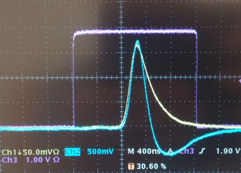
8 Generic signal produced by the PMT-premaplifier combo viewed by
an oscillator. Yellow: the original signal inverted. Blue: amplified
signal with -10x gain by a time filtering amplifier. Purple: gate signal
used in Section 5.2. . . . . . . . . . . . . . . . . . . . . . . . . . . . . 28
9 HIGH-LOW graph formed by 2-channel method. The dashed lines
box the background region and show a linear reference line passing
through the origin and background data point. . . . . . . . . . . . . . 32
10 Some of the spectra used for the channel analysis. The grey dashed
lines show the location of energy window dividing channels. . . . . . . 32
11 Illustration of the effects of different sample rates. . . . . . . . . . . . 34
12 The mean for each mean location with different sample intervals. . . . 34
13 Different radiation sources measured with the PS using 2-channel
method. All data is offset for a single background point (grey circle).
Grey dashed lines are linear and only for reference. . . . . . . . . . . 36
14 Moving mean graphs of the HIGH-LOW data shown in Fig. 13. All
data is offset for a single background point (grey circle). Grey dashed
lines are linear and only for reference. . . . . . . . . . . . . . . . . . . 36
15 The LOW channel of a measurement of a moving vehicle. . . . . . . . 37
16 The measurement locations and their labels used in the defect probing
measurements. . . . . . . . . . . . . . . . . . . . . . . . . . . . . . . . 39
17 Results from the probing measurement using 241 Am source . . . . . . 40
18 Results from the probing measurement using 137 Cs source . . . . . . . 4012
19 Part of the energy spectra measured near PMT using collimated
241
Am source. Labels are coordinates as in Fig. 16. . . . . . . . . . . 41
20 Part of the energy spectra measured near PMT using collimated 137 Cs
source. Labels are coordinates as in Fig. 16. . . . . . . . . . . . . . . 41
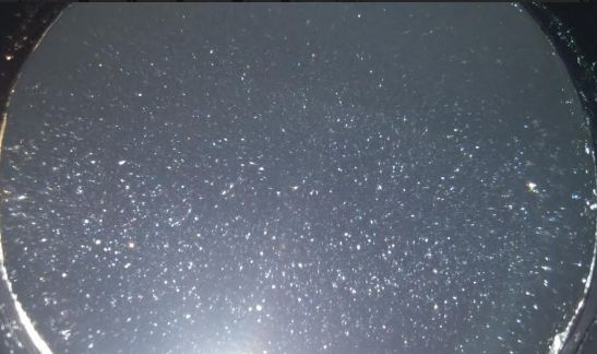
21 A photograph of a similar PS showing visible defects caused by ageing
effects. The defects are also within the scintillation material and not
only at the surface. . . . . . . . . . . . . . . . . . . . . . . . . . . . . 43
22 The scintillator setup for coincidence measurements. The radiation
source is placed in the source holder (left image) which is placed be-
tween PS and the secondary scintillator (right image). The secondary
scintillator in the right picture is the 3" LaBr3 . . . . . . . . . . . . . . 45
23 The measurement setup for attenuation length measurements on the
field. The PS is inside the blue metal casing upright and the hanging
1.5" LaBr3 is facing the monitoring side. . . . . . . . . . . . . . . . . 46
24 The delayed signals from (Yellow) PS before the amplifier, (Teal) PS
after the amplifier and (Purple) the ”gate signal” at the end of LaBr3
signal line. . . . . . . . . . . . . . . . . . . . . . . . . . . . . . . . . . 46
25 The measurement equipment and module wiring used for the coinci-
dence measurements. The LaBr3 scintillator in the picture is the 1.5"
BrilLanCe 380. . . . . . . . . . . . . . . . . . . . . . . . . . . . . . . 47
26 Spectra from 1.5" LaBr3 with and without self-gating 137 Cs source, as
well as the background spectrum for reference. The red curve shows
the region to be used as gate. . . . . . . . . . . . . . . . . . . . . . . 47
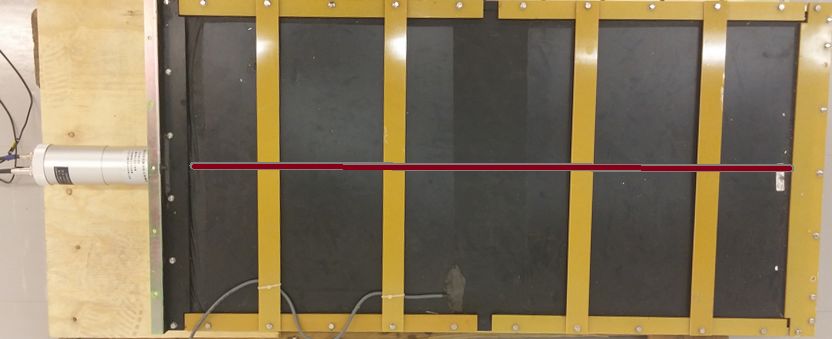
27 The attenuation length spectra are gathered along the red line shown. 48
28 LaBr3 spectra of the different gate locations measured using the self-
gating technique. Inset: broader x-axis from channel 1 to 1800. . . . . 49
29 PS spectra acquired using the gates shown in Fig. 28. The ungated
spectrum is scaled by a factor of 7.5e-3. µ and M corresponds to the
peak’s location (channel) and height (cps), respectively. . . . . . . . . 50
30 PS spectra gated at and right from the backscattering peak, and
their difference. Gaussian fits for the normally gated and subtracted
spectra and linear fit for the right-shifted gated spectra with their
parameters are also shown. Region of interest (ROI) for the fits are
marked with thick circles. . . . . . . . . . . . . . . . . . . . . . . . . 51
31 The means µ gathered from all measurement sets with exponential fits. 54
32 The FWHM’s gathered from all measurement sets. . . . . . . . . . . 54
33 The relative resolutions gathered from all measurement sets. . . . . . 55
34 Examples of the GC-function with varying variances for a 662 keV
gamma. . . . . . . . . . . . . . . . . . . . . . . . . . . . . . . . . . . 57
35 GC-function fitted to background-subtracted 133 Ba, 137 Cs and 60 Co
spectra. Lighter lines: measurement data. Darker lines: the GC
fit. Black dashed lines: unconvoluted Klein-Nishina. Grey vertical
dashed lines: ROI limits. . . . . . . . . . . . . . . . . . . . . . . . . . 6213
36 Energy calibration curve obtained from the fits shown in Fig. 35.
The red circles show the locations of the Compton edges of the fits. . 62
37 The resolution calibrations obtained from the fits shown in Fig. 35.
The purple point from manual 208 Tl fitting was not used for this
calibration. . . . . . . . . . . . . . . . . . . . . . . . . . . . . . . . . 63
38 Fits of the 208 Tl area in the background spectrum using parameters
obtained from the initial fits (Fig. 35) and by manual parameter
adjustment. . . . . . . . . . . . . . . . . . . . . . . . . . . . . . . . . 63
39 Fit for background subtracted 40 K spectrum using parameters from
the initial fits (Fig. 35). . . . . . . . . . . . . . . . . . . . . . . . . . 64
208
40 Tl-stripped background spectrum (from Fig. 38) and background
subtracted 40 K spectrum (from Fig. 39) . . . . . . . . . . . . . . . . . 64
41 GC-function fitted to multiple sources measured with 1.5" LaBr3 . . . 65
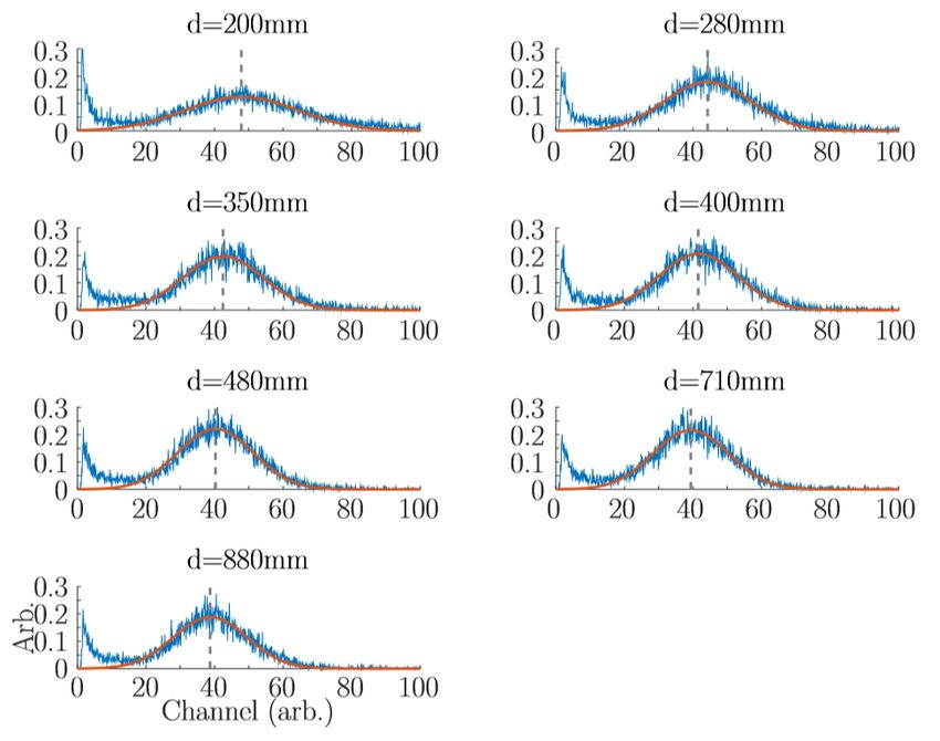
42 The spectra measured from different distances using the 1.5" LaBr3 . . 75
43 The spectra measured from different distances using the 3" LaBr3 . . . 76
44 The spectra measured from different distances using the 1.5" LaBr3
on field from the first PS. . . . . . . . . . . . . . . . . . . . . . . . . 77
45 The spectra measured from different distances using the 1.5" LaBr3
on field from the second PS. . . . . . . . . . . . . . . . . . . . . . . . 7814
15

List of Tables
  1   Properties of some commercially available plastic scintillators [16, 12]        26
  2   The parameters of the fits shown in Fig. 31 . . . . . . . . . . . . . .         53
  3   GC-function fit parameters obtained in Fig. 35. SE = standard error.            61
  4   Means and FWHMs gathered from coincidence measurement spectra
      presented in Appendix B. In Field measurements the 1.5" LaBr3 was
      used. . . . . . . . . . . . . . . . . . . . . . . . . . . . . . . . . . . . .   79
16
17

1       Introduction

Efficient monitoring of the flow and movement of nuclear and other radioactive
materials is a vital point in maintaining national security. With an increase of
various users of radioactive materials – e.g. in nuclear power, medical field and
industry – the risk of improper handling of artificial radionuclei becomes relevant.
The legal flow of radioactive materials has also grown accordingly. In a mission to
maintain the national security customs have a vast arsenal of radiation detectors for
vehicle and pedestrian scanning at border crossing points. The primal inspection
stations are typically stationary plastic based radiation portal monitors.
These monitors are usually positioned on the side of the lanes to scan vehicles and
pedestrians in a fast rate and their task is to give an alarm in case they detect
radioactive substances and materials. Plastic scintillators (PS) are usually selected
for this task because they are a fast material, and for their efficient bulk produc-
tion, high sensitivity due to their achievable large sizes, and cheap material costs.
The main limitation of PS is poor energy resolution, i.e. the ability to distinguish
different radiation energies, which challenges the source identification methods.
When using PSs only as rough counters, a big portion of radiation alarms are so
called nuisance alarms. These are real alarms caused by naturally occurring radioac-
tive materials (NORMs) e.g. natural uranium or thorium in porcelain and construc-
tion aggregates. Because a moderate amount of NORM substances are allowed the
further inspection processes of NORM containing loads is in most cases unnecessary.
Specialized algorithms are therefore needed to distinguish NORM loads, forcing the
limited resolution of a PS to be utilized.
As a secondary motivation for this thesis, the lifespan of a PS is roughly 10 years.
During its lifetime PS’s detectability decreases and requires recalibration and even-
tually replacement. Furthermore, it has been shown [1] that different PSs age in-
dependently which allows the replacement of individual radiation monitors over a
wide timespan. To continue PSs operation over the the expected replacement date
will also save expenses especially since plastic based radiation monitors are usually
part of large scale systems1 .

    1
  As of October 2016 there was 1400 radiation portal monitors stationed in United States of
America most of them containing 4 PSs [9].
18
19

2       Theoretical background

2.1     Photon interactions in plastic

As a gamma ray interacts with scintillation material secondary photons are emitted.
The most probable type of interaction depends on the energy of the incident gamma
and the mass number of scintillation material as shown in Fig. 1. For our purposes
we concentrate on low-Z region as the plastic scintillators are mainly hydrocarbons.
For Z < 20 the Compton effect is dominant at the energy range of 100 keV – 10 MeV,
which covers almost the whole range of gamma radiation from common radioactive
nuclei, missing out only the lowest energies 2 . Pair production is highly improbable
in our energy range of interest and thus not discussed from this point onwards.
The probability coefficient τ for photoelectric absorption is proportional to Z n /E 3.5
[6, p. 49], where Z is the mass number of the absorber, n is a constant between
4 and 5 and E is the energy of the incident photon. This model of τ creates a
straight descending line in log-log scale when plotted as a function of energy E. We
can observe this from the behaviour of mass attenuation coefficient µ/ρ graph of
a common scintillation material vinyl toluene shown in Fig. 2. The attenuation
coefficient µ is the sum of the probabilities from photoelectric absorption, Compton
scattering and pair production, and ρ is the medium’s density. Because the linear
region of the graph changes significantly at roughly 50 keV and according to the
model the component of the photoelectric absorption becomes very small, we can
assume that all the interactions undergone by photons in the scintillation material is
via the Compton scattering. It is worth mentioning here that µ is also the reciprocal
of attenuation length λ which describes the distance a gamma beam has to propagate
within the medium for its intensity to drop to one e’th.

    2
    The highest gamma energies considered in this thesis is 4.4 MeV from α-Be neutron source
and fission gammas up to 5 MeV.
20 Figure 1. Probability scheme for different gamma scattering interaction prob- abilities showing equality borders where the probability of neighbouring inter- actions are equal. Figure from Ref. [6]. Figure 2. Mass attenuation coefficient data µ/ρ for vinyl toluene and modelled photoelectric τ /ρ and Compton scattering σKN /ρ components. Ki are scaling constants and dσKN /d(cos θ) the Klein-Nishina formula [6]. Data from Ref. [10].
21

2.2    Compton scattering

In Compton scattering part of the initial gamma’s energy E is transferred to the
scattered electron according to equation
                                                 E
                               E∗ =         E                                      (1)
                                      1+   m e c2
                                                  (1   − cos θ)

where E ∗ is the energy of the scattered gamma, me c2 the rest mass of an electron and
θ is the gamma’s scattering angle. The rest of the energy, T = E − E ∗ , is transferred
to the electron from which the gamma scattered. The Compton scattering process
is illustrated in Fig. 3.
The probabilities for each scattering angles are not equally distributed. The differ-
ential cross section for an initial gamma of an energy E to scatter in an angle θ, per
atom, is given by the Klein-Nishina formula
                                       2
                    dσKN        E∗            E∗  E

                         = Zr02                  + ∗ − sin2 (θ) /2                 (2)
                     dΩ         E             E   E
where dσKN /dΩ is the differential cross section for a scattering angle element, Z the
number of electrons per atoms (or the atomic number of the absorber material),
r0 the classical electron radius, and E ∗ the photon’s energy after the scattering as
given by Eq. (1). For a free electron Z = 1.
When the energy transferred to the scattered electron T is of interest, such as in
case of scintillators, one can use the reformed Klein-Nishina formula
                                                                          !
               dσKN   Zr02 π 1         S2         S     2

                    =        · 2 +             +     S−                            (3)
                dT         2
                      me c α       α (1 − S)
                                    2        2   1−S    α

where α = E/me c2 , and S = T /E. This differential cross-section is directly pro-
portional to the probability distribution for the scattered electron to have kinetic
energy T .
For a derivation of equations (2) and (3) see Appendix A.1.
As the scattered gamma’s energy reaches its minimum at a 180◦ backscattering, the
maximum values for T and S are
                                                                 2
                         ∗             1        2α          2 2α
           Tmax = E −   Emin   =E−E        =E        = me c                        (4)
                                    1 + 2α    1 + 2α         1 + 2α
and
                                              2α
                             Smax = Tmax /E =       .                       (5)
                                            1 + 2α
The energy Tmax is called as Compton edge energy and corresponds to the highest
energy deposited by a photon in Compton scattering.
22
Figure 3. Illustration of the Compton scattering process.
2.3 Scintillation and energy level structure in plastic
The Compton scattered electron will eventually interact with other electrons of the
scintillation material creating molecular excitations. As these excited states return
to ground level so called secondary or scintillation photons are emitted. In some cases
the secondary photon is of the same energy required to excite the molecule resulting
into so called self-absorption. For a photon to propagate within the scintillation
material these scintillation photons must have a lower energy. In organic scintillators
this is acquired by the molecules’ energy structure.
To minimize this self-absorption in plastic and other organic scintillation materials
the molecular energy level structure with so called π-orbitals are of interest. An
energy level scheme for these orbitals are shown in Fig. 4. The energy levels are
indexed as Si,j , where i corresponds to the excitation level and j its vibrational
sublevel. When the electron is excited to some non-zero vibrational level of an
excitation state (say, S1,1 ), it quickly loses the vibrational energy in the form of heat
and moves to the zero vibrational state of that excited state (S1,0 ) in the matter of
picoseconds. From here the electron can decay into any vibrational states (~10−8 s)
of the lower energy levels (e.g. S0,1 ) emitting a secondary photon. This vibrational
state again quickly decays into zero-vibrational state (S0,0 ). [6]
For the sake of completeness, the molecule can also excite into triplet states. Because
their lifetime is much longer (> 10−4 s) and as the time window of one gamma
interaction is of the order of 100 – 1000 ns (discussed further in section 3.2) the
triplet states do not contribute to our measurements and are thus ignored.
The benefit of the π-structure is that the emitted photon does not have enough
energy for self-absorption if the decay happened via a vibration state. Therefore23
Figure 4. π-structure of energy levels in organic molecule.
the emission spectrum gets shifted towards longer wavelengths with respect to the
absorption spectrum. This is commonly called a Stokes shift.
The Stokes shift of the base material, or solvant, alone is usually not enough and
is enhanced with different dopants to further minimize self-absorption. Different
dopands are chosen according to desired applications for the material. Some common
dopants are p-terphenyl, PPO and POPOP. The overlapping of absorption and
emission spectra of some commercial polyvinyl toluene (PVT) based scintillators
can be observed in Fig. 5. While the base material is the same (PVT) the dopants
affect greatly to the optical spectra.24 Figure 5. Absorption and emission spectra of polyvinyl toluene based wave- length shifters. Figure from Ref. [16]. 2.4 Radioactive sources After a nucleus has undergone a decay or has been created in a nuclear reactions, the daughter nucleus can be in excited states. Given that no further processes were undergone, these states further decay into lower excited states and eventually to their ground states. During these processes gamma radiation is emitted which are characteristic to each nuclei. Detecting the characteristic gammas is in most cases the main identification method. While not relevant in this thesis, fission sources and β-emitters also radiate gammas. In fission the daughter nuclei can have varying kinetic energies and the prompt gammas emitted have a continuous energy spectrum. Electrons from β-emitters, most notably 90 Sr and 90 Y, also create a continuous gamma spectrum as they travel in a medium via bremsstrahlung. There is a variety of radioactive sources. 241 Am is a very common calibration source for it decays only via α-decay and mainly (84.6%) into an excited state of 237 Np with an energy of 59.5 keV. While 241 Am has a half life of 432 years, the lifetime of the excited state of 237 Np is only 67 ns. Because the lifetime of 237 Np is of the order of 106 years the 59.5 keV is the dominant gamma radiation energy of an 241 Am source. Another common source, 137 Cs, β-decays into ground state or an isomeric level of 137 Ba with an energy of 661 keV. Some sources, including 241 Am, decay further and thus emit multiple gammas with different energies. One of the longest common decay chain starting from the NORM 238 U has 14 steps before reaching the stable 206 Pb where most of the steps emit gammas, including the 2614 keV gamma from the decay of 208 Tl. Because the lifetimes of the intermediate nuclei in this so called uranium series vary from 105 years to few seconds, the 238 U-source has a high number of characteristic gammas. Lastly, a beryllium-based neutron emitters such as 241 AmBe undergoe a fusion process 9 Be(α,n)12 C where the created carbon nucleus can be at its excited state of 4.4 MeV. [15, 8] Most of the gamma energies from radioactive sources of our interest fall between the 59.5 keV from 241 Am and 2614 keV one from 208 Tl. Some other radiation sources
25

are also used to get intermediate gamma energies, where most important to this
thesis are 133 Ba (356 keV), 137 Cs (661 keV), 60 Co (1173 keV and 1333 keV) and the
important NORM, 40 K (1460 keV).
26
3 Scintillator system
In this section the scintillator hardware used in our measurements is described.
Because the signal processing setup varies between measurements the complete setup
with the modules used are described individually in each section. All hardware and
software are also listed at the end of the Reference section.
3.1 Scintillation material
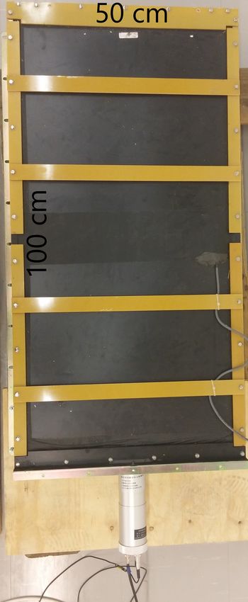
The plastic scintillator shown in Fig. 6 is used in our measurements and is from
a commercial radiation monitor. This unit is roughly ten years old and has been
in operational use in an environment with rough weather conditions including high
humidity and temperatures varying from -30◦ C to +30◦ C annually. The scintillator
casing was never opened and is assumed that the scintillator material was wrapped
in a reflective foil and then to a black plastic wrapping. The scintillator material is
assumed to be polyvinyl toluene (PVT) which is the base material in most common
plastic scintillators. Different plastic scintillation materials vary mainly in operative
appliances, decay time, luminescence, sensitivity and absorption-emission spectra,
all of which do not affect our measurement methods and results significantly. All
common plastic scintillation materials also fulfil the requirements and assumptions
made in this thesis. Properties of common plastic scintillation materials are shown
in Table 1. As mentioned earlier, the attenuation length is the distance after which
the light’s intensity has dropped to one e’th.
Table 1. Properties of some commercially available plastic scintillators [16, 12]
Name Base Density Refractive Decay Emission Max. Attenuation
(g/cm3 ) index constant wavelength length λ
(ns) (nm) (cm)
EJ-200 PVT 1.023 1.58 2.1 425 380
EJ-204 PVT 1.023 1.58 1.8 408 160
EJ-208 PVT 1.023 1.58 3.3 435 400
IHEP )
– SC-201
PS 1.05 1.59 3.0 420 200
– SC-205
PVT= polyvinyl toluene, PS = polystyrene27 Figure 6. The top view of the plastic scintillator mainly used for our measure- ments 3.2 Photomultiplier tube The secondary photons emitted via scintillation propagate eventually to a photo- multiplier tube (PMT). PMT consists of three main components: a photocathode, a dynode line and an anode. The working principle is illustrated in Fig. 7. When a photon hits the photocathode of the PMT, a photoelectron gets released. This electron is then led through a series of dynodes each in a higher potential than the previous one. Upon impacting a dynode an electron can release additional electrons from it multiplying the number of electrons accelerated towards the next dynode. This creates a avalanche of electrons all which eventually reach the last dynode named anode. The current reaching anode creates a signal which is fed to the signal processing unit. In practice PMT has some capacitance since the anode gets charged during a period of time to discharge afterwards. Like for all capacitors, the time constant varies by unit, but in this thesis the time during which the charge decays from the maximum to one e’th is the order of 100 – 1000 ns. The scintillator material block is connected to a PMT-preamplifier combo (PP) with optical grease without additional light guide. For each scintillation event the PP gives a voltage pulse of negative polarity with an amplitude ranging from -10 mV to -2 V. An amplitude of -100 mV corresponds roughly to 530 keV. A general shape of this signal is shown in Fig. 8. The signal has a width of few hundreds of nanoseconds as described earlier depending on the amplitude of the signal. The PP is cased in a metallic cylinder which is visible at the left end of the scintillator shown in Fig. 6.
28

 Figure 7. Illustration of the working mechanism of a PMT. Figure from
 hamamatsu.magnet.fsu.edu.

 Figure 8. Generic signal produced by the PMT-premaplifier combo viewed by
 an oscillator. Yellow: the original signal inverted. Blue: amplified signal with
 -10x gain by a time filtering amplifier. Purple: gate signal used in Section 5.2.
29

4     Operative usage

In the past, plastic scintillators were mainly used as rough counters to detect a
presence of a radioactive source. The alarms resulting from NORMs, sometimes
referred to as nuisance alarms, are very frequent due to the high abundance in
shipped cargo. While the radiation is indeed present, in most cases it does not
exceed the allowed concentration or strength limits creating unnecessary work for the
inspection personnel. This is one of the reasons why better resolution devices, such
as sodium iodine (NaI) detectors, have gained popularity in order to distinguish the
NORM loads. Still, plastic scintillators can be set up to give a rough estimate of the
radioactive sources. Usually this is done by dividing the signals into bins according
to their amplitudes. This is called energy windowing as the signal amplitude is
proportional to the energy disposed to the PS by the initial photon. Increasing
the number of energy windows eventually leads to spectroscopy but using only few
energy windows keeps the system simple and robust. We will study the advantages
and disadvantages of the two channel method, and suggest ways for measurement
analysis.

4.1    Two-channel method (2C)

Artificially made radioactive nuclei radiate mainly at low energies, whereas the low-
est gamma energy for NORMs used for nuclide identification is 1460 keV photopeak
from 40 K. This allows us to make a simple estimation, stating that as long as a
source radiates only gammas with energies below 1460 keV, it is artificial or other-
wise worth investigating. This statement is very straightforward to implement to
the hardware while allowing flexibility between individual radiation monitors.
While the Compton scattering from the PS creates a range of energies that are read
as pulse signals, each gamma can transfer a maximum of an 180◦ backscattering.
Since the signal from PMT is proportional to the energy transferred to PS one only
needs to probe whether a present source creates signals above a certain reference
signal or not.
30

4.1.1   2C: Working principle

The signal processing can ultimately be done by dividing the voltage signal from
PMT with two comparators. The reference voltage of the first comparator, V1 ,
should be set low only to cut off the electric noise. The reference voltage of the
second comparator, V2 where V2 > V1 , is used to divide the bins. The outputs are
then led to individual pulse counters.
For the sake of simplicity, since signals over V2 are passed by both comparators, one
should make the counters anti-coincide with each other. This can be done by either
subtracting the counts of higher window from lower window or by implementing
logical gates. As a result, the first counter only detects signals between voltages V1
and V2 and the second counter detects signals over V2 . The second counter was left
without an upper limit.
Because the lower voltages correspond to lower gamma energies, we will herein call
the first counter the LOW channel. Similarly, the second counter is called the HIGH
channel. The term channel is used for convenience as it is more commonly used when
the number of energy windows increase.
A HIGH/LOW ratio (or its reciprocal) has been discussed in early literature [2] but
it has a tendency to miss out information. As the radiation source becomes stronger
the count rates start to skew towards HIGH channel due to the limited resolution
of PS. Therefore the concept of total count rate, HIGH+LOW, has to be induced
to the model as well. Further, if the source is weak compared to the background
the ratio does not change significantly. The debatable improvement of background
subtraction in this case could result in division by zero.
Our analysing method presents the count rates in a simple double logarithmic graph
where the HIGH (LOW) channel count rate is on x(y)-axis. This provides a quick
visual of the measurement results while maintaining the contrast to the background.
It uses the advantage of the unique spectra created by different radiation sources
and the changes in count rates as the strength of the source relative to the detector
changes.

4.1.2   2C: Measurements and results

The first task is to calibrate the reference voltages V1 and V2 . This can be done
using 241 Am and 137 Cs sources as they are very common industrial sources and have
a relatively long lifetime. The lower threshold, V1 , should be calibrated to reduce
the electric noise as much as possible while still passing through most of the signals
created by 241 Am source. One should also note that below the 59.5 keV gamma
of 241 Am lies some common radiation sources, such as 35.5 keV from medical 125 I
(T1/2 = 60 days). The voltage V2 should utilized to distinguish NORM sources. A
prominent location is to set it high while maintaining the visibility opf 40 K.
31

In our setup the spectra of different radiation sources were measured with PS. The
signal from PP is fed via an inverter (Philips Scientific, model 740) to a multichannel
analyzer (MCA, Ortec 927) which is connected to a computer with appropriate
software. We simulated the HIGH and LOW channels by integrating the count rate
along specific channel ranges. This is justified because a channel in MCA spectrum
is linearly proportional to a specific voltage amplitude range in PMT. Using an MCA
allows us also to create a visual picture of where the reference voltages are located
in the energy spectrum.

The key points in the calibration process are to first maintain the detectability of
low energy source and to distinguish 40 K and 60 Co sources as they have very similar
energies. 133 Ba with a 356 keV photopeak was used as a low energy source in our
calibration. The channel ranges for LOW and HIGH energy windows were selected
to be channels 18 and 80, and because the MCA was operated in 4096 channel mode
with voltage range from 0 V to +10 V, the corresponding reference voltages are 44
mV and 195 mV, respectively. The radiation sources used in the experiment were
measured from multiple distances ranging from 9 cm to 300 cm depending on the
source to simulate different intensity sources. Additional amplifiers were not used
as the ones available had a tendency to induce artefacts during the experimenting
phase.

The resulting HIGH-LOW graph is shown in Fig. 9 and some of the the MCA
spectra with the used channel limits in Fig. 10. The most visible anomaly in Fig. 9
is the location of 133 Ba data points. A closer inspection in the spectrum graph (Fig.
10) reveals that the decrease of count rate with respect to background in HIGH
channel is mainly due to the statistical error near channels 80–100. This is a great
visual hint of the uncertainty region around the background in which an increase
in either channel can and should be considered to be within the noise region. The
leaning towards the HIGH channel can be seen from the 137 Cs and natural uranium
(NU) plots as well as higher energy sources (e.g. 152 Eu, not shown completely).

Each radiation source has a characteristic HIGH/LOW ratio and the stronger the
source is the further it is from the background point. Varying the intensity creates
paths, source lines, in the HIGH-LOW graph. These lines may vary depending
on the casing shielding the radiation monitor. By inserting a small margins one
can create regions for each source denoting the corresponding source’s data region.
Changing the channel dividing point (grey lines in Fig. 10) will result in changes of
source lines in Fig. 9 which allows one to manipulate the proximities of source lines.
As an example, for NORM identification the 40 K and 232 Th sources will be treated
the same which makes their source line overlap insignificant. In turn, the overlap
between 40 K and 60 Co should be minimized as 60 Co is an industrial source, which
requires further investigation.

Even while the energy calibration will be different for each PS, if one desires to cre-
ate a HIGH-LOW calibration for multiple plastic radiation monitors with identical
setup referring a calibration spectra should be sufficient instead of measuring all
32

 Figure 9. HIGH-LOW graph formed by 2-channel method. The dashed lines
 box the background region and show a linear reference line passing through the
 origin and background data point.

 Figure 10. Some of the spectra used for the channel analysis. The grey dashed
 lines show the location of energy window dividing channels.
33

sources with all PS. A reference spectrum can be a background spectrum as long
as the shape of the background spectra are the same, or alternatively a background
subtracted 137 Cs spectrum. The difference in the energy resolutions – the capability
to distinguish different gamma energies – between multiple PS can be speculated to
affect mainly the leanness of the source lines as the intensity of the source increases.
It is noteworthy that the counts from the low-end of an energy window dominate
the high end counts. Considering the 40 K spectrum in Fig. 10, the ratio between
40
   K count rate and background count rate are 1.11 and 1.27 at channels 20 and 70,
respectively. Moving the lower limit of LOW window to higher channels will thus
enhance the visibility of a 40 K source. This is because the count rate is higher at
lower channels but has smaller significance for 40 K. Dividing the energy windows
to smaller sub-windows directly enhances the detectability since the significance of
count rate increase along the whole energy region becomes more equal3 .

4.2       Channel detectability enhancement

When measuring traffic with the radiation monitor, the signal from PS is fed to
comparators and the number of counts from both comparators within a fixed time
interval is recorded. The reciprocal of this recording time is called the sample rate.
While the high processing speed of PS allows high sample rates up to the order of
100 Hz, decreasing the sample rate reduces the fluctuations in the count rates. As a
drawback, with low sample rates the overall detectability decreases for fast passing
sources. Varying velocities of passing vehicles demands play with the sample rates
for individual radiation monitoring system. A simulated illustration of this effect is
shown in Fig. 11 where the passing source is represented by a Gaussian shape with
added white noise.
The detectability can be enhanced also by understanding that the change of count
rate due to a moving radiation source is well-behaving. While the fluctuations are
well visible in high sample rates (the 1000 Hz line in Fig. 11) the count rate does
increase on average when a source is present. Therefore by analysing the progression
of the mean we can detect the signal induced increase in our count rate graph. This
moving mean graph is done by plotting the mean of all counts within an expanded
time interval for all sample points as the mean location 4 . An illustrating graph
from the simulation above is presented in Fig. 12.

  3
      Increase of the count rate by 10 cps has higher significance the lower the background is.
  4
      This is a convolution between the data and a rectangular function.
34
Figure 11. Illustration of the effects of different sample rates.
Figure 12. The mean for each mean location with different sample intervals.35
4.3 Practical appliance
A PS similar to this thesis’ was positioned next to a road with vehicle traffic. In
our setup the sample rate was set to 20 Hz with a 20 sample (1 second) mean
span. Stationary radiation sources were first measured in order to achieve a proper
calibration. In the lack of a feasible 40 K source the V2 is set just above the limit where
the 137 Cs source becomes visible, so that the voltage should correspond to roughly
600–800 keV. After calibrations an unknown source was measured. The background
was also measured individually for all measurement set right before measuring the
source.
The resulting HIGH-LOW graphs for the sources are shown in Fig. 13 and the
moving mean graph with a 1 second interval in Fig. 14. All data has been offset so
that the background data points become equal for the sake of source comparison.
This can be done as the background can be arbitrary as long as it is well known,
while the count rate increase from a stationary source is constant5 . The 133 Ba source
being directly above the background is a strong industrial source indication, but has
big fluctuations in the HIGH channels probably due to background. Data from
137
Cs, 60 Co and unknown sources can be easily divided with linear lines and after
consulting Fig. 9 the unknown source can be declared as a moving 40 K source.
Because we did not measure 40 K systematically, the declaration requires further
experimenting to locate source lines and regions.
During a radiation alarm the graphs in Fig. 14 can provide a quick insight for
types of radiation sources present. Most importantly, separating NORM sources
allows different procedures and reduces nuisance alarms. The alarm levels can be
ultimately defined with the background level and the regions to which the source
lines get drawn.
A measurement of a vehicle without a radiation source is shown in Fig. 15. The
background’s count rate visibly decreases as the vehicle passes the radiation monitor.
This is due to the vehicle blocking some of the background radiation that would
otherwise be detected by PS. This effect, commonly called ”vehicle shielding”, should
be taken into consideration when setting up vehicle radiation monitor systems and
especially the alarm algorithms.
5
The background level does affect the statistical detection sensibility and is relevant when
considering alarm levels36 Figure 13. Different radiation sources measured with the PS using 2-channel method. All data is offset for a single background point (grey circle). Grey dashed lines are linear and only for reference. Figure 14. Moving mean graphs of the HIGH-LOW data shown in Fig. 13. All data is offset for a single background point (grey circle). Grey dashed lines are linear and only for reference.
37

      Figure 15. The LOW channel of a measurement of a moving vehicle.

4.4    Multichannel method

In order to make the source identification more accurate one can divide the channels
further. With the third energy window one can try to separate a specific nuclide, e.g.
40
   K, or to divide the LOW channel into two. In general, as one adds more channels,
the individual ratios between the channels become more complex and unique to
different sources. One prominent energy window would be to distinguish α-Be and
fission neutron sources by probing gammas at up to 4 MeV [3] since most radiation
monitors also have separate neutron detectors. While all neutron alarms should be
investigated, a preliminary information for a possible fission source, such as 252-Cf,
is valuable.
Because the number of possible values, sums and ratios increases rapidly with the
number of energy windows it can be feasible to create new methods for identification.
Increasing the number of energy windows will eventually lead to a spectrometric
analysis. One tool for spectrometric nuclide identification is a fitting procedure
which is an application of the numerical method presented in 5.3. Here, a specific
function is fitted to the background subtracted spectrum resembling the Compton
continuum of a photopeak. From there one can obtain the original photopeak energy
and proceed to a regular nuclide identification process.
38
5 Characterization techniques
Three different techniques were applied to probe the PS’s condition and for calibra-
tion purposes. In section 5.1 we scan through PS with a collimated source in search
of defects or other structural non-uniformities. Section 5.2 presents a method to
evaluate the attenuation length of the scintillation material that doesn’t require any
disassembling of the radiation monitor. Finally, in section 5.3 we make use of the
Gaussian distributed energy components and create a numerical fitting method for
energy and resolution calibrations which can be utilized to nuclide identification.
5.1 Defect probing
The uniformity of the scintillation material is checked to detect any major defects
such as cracks or localised dusky spots in the scintillation material. Defects of this
nature all result in significant light yield loss in the scintillation material which in
turn reduces the efficiency of the radiation detector. The defects can be induced
both in the manufacturing process and due to ageing effects.
One non-destructive method is to scan the whole scintillator over a matrix. This
setup is also field-operable as it doesn’t require disassembling of the radiation mon-
itor as long as the gamma rays can sufficiently penetrate the casing of the monitor.
5.1.1 Probing: Measurement setup
The signal from the PS is led through an inverter to MCA similarly as in Section
4.1.2. MCA is used to get spectra from every measurement only in case we need
additional information, but most of the analysis can be done by simple counters.
The radiation sources used are 137 Cs and 241 Am where the former is used for internal
and latter for surface probing. The measurement time was 120 seconds per location.
We can calculate the absorption probability P according to the equation
P = 1 − e−(µ/ρ)x (6)
where µ/ρ is the mass attenuation coefficient, x = d · ρ is the mass thickness, ρ the
density and d the depth. Using the data from [10] shown in Fig. 2 in Section 2.1,
the mass attenuation coefficient µ/ρ is 0.1893 cm2 /g at 59 keV and 0.084 cm2 /g at
662 keV. Assuming the density of 1.023 g/cm3 from Table 1 at Section 2.1 we can
compute that 50% of the gammas with energies 59 keV and 662 keV have undergone39
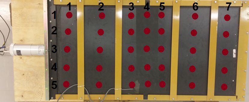
Figure 16. The measurement locations and their labels used in the defect
probing measurements.
absorption in depths 3.58 cm and 8.06 cm, respectively. For comparison, the PS
case thickness altogether is 11 cm including a probable lead shield on the back side.
The radiation sources were collimated using a lead cylinder with roughly 1.5 cm
thick wall and a 2 cm diameter hole at the bottom. The collimated source was
measured in different locations over the PS. By measuring the cps in each location
we can form a contour map which reveals the information from the light propagation
inside the scintillation material. Due to a constant background, there is no need for
background subtractions to normalize separate measurements6 .
The probing was done in a 5-by-7 matrix as shown in Fig. 16.
5.1.2 Probing: Results
From the 241 Am and 137 Cs measurements we can create contour maps showing the
total count rates. These are shown in Fig. 17 and 18, respectively. From the figures
one can easily conclude that the count rate decreases as we go further from the
PP, which is expectable as light travels further through medium. In both cases the
corners at the PP’s end are significantly dimmer than in the middle which shows
the lack of light guide between the scintillation material and PMT. In the case of
241
Am, there is a clear decrease in count rates at the edge in the middle of the PS
(location 5,4) which is exactly the location of an assumed thermometer. The whole
middle part has lower count rates in general implying additional material between
the source and PS. Note that these effects are not visible with 137 Cs measurements
as its gammas penetrate the surface relatively easily. On the other hand, the effect
of being closer to the edges are far more visible with 137 Cs.
6
Our signal is also well distinguishable from the background as discussed at the results section.40
241
Figure 17. Results from the probing measurement using Am source
137
Figure 18. Results from the probing measurement using Cs source41 Figure 19. Part of the energy spectra measured near PMT using collimated 241 Am source. Labels are coordinates as in Fig. 16. Figure 20. Part of the energy spectra measured near PMT using collimated 137 Cs source. Labels are coordinates as in Fig. 16.
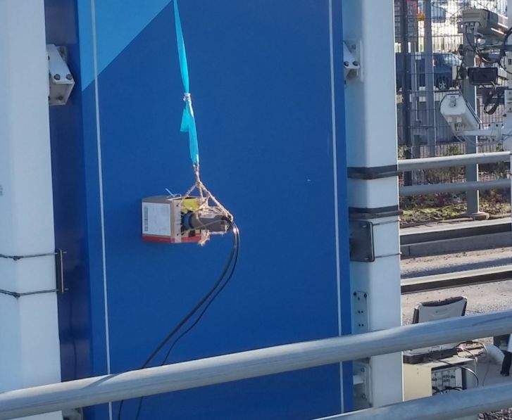
42

137
   Cs measurement shows unexpected behaviour where the count rate drops as we
get closer to the PMT on the central line. From the measurement spectra shown
in Fig. 19 and 20 it is clear that the 137 Cs spectra becomes anomalous near the
PMT. Possible cause is that a significant portion of the gammas can reach the PMT
bypassing the scintillation process. Thus data from these locations should be taken
cautiously. Similar, but less significant, effect is visible also in case of 241 Am.

5.2    Attenuation length using coincidence method

As the plastic ages it becomes foggy due to small defects and other damage caused
by different ageing processes. This reduces the attenuation length especially for
the scintillation photons, the length of which light can travel through the medium
until its intensity reduces to one e’th. When ageing less photons reach the PMT
created by the same initial gamma energy, which in spectrum analysis can be seen
as a spectrum scaling towards zero. While this can be compensated by amplifiers,
the major problem arises from the unideal electronics. Artefacts at the low voltage
region due to e.g. bad grounding are always relative to the scintillation signals and
need to be cut off for proper spectrum or energy window analyses. Ultimately, as the
scintillation material ages and the signal voltages become lower, low energy sources
such as 241 Am cannot be feasibly detected.
The countermeasure is to simply replace the plastics to new ones. In case of mul-
tiple radiation detectors the cost of replacing all the plastics might cumulate to a
significant expense. Thus it is convenient to monitor plastics’ condition and replace
them only when needed. Individual plastics also age at a different pace, so replacing
only the unusable ones also evens out the expenses on longer period.
A way to monitor plastics’ condition is to measure their attenuation lengths over
their lifespan. An affordable and field-deployable method is presented here and also
shown to work on field without disassembling the radiation monitor at all. Another
characteristic to probe is the (relative) energy resolution R, which is defined as
the ratio of the full-width-half-maximum (FWHM) and the mean µ of measured
spectrum for single-energy scattering events.
The goal of this experiment is to probe the duskiness of the scintillation material.
Different environmental and radiation deduced ageing effects from have been shown
to create defects in the surface and within the scintillation material. Because the PS
used in this thesis is an old one these effects are assumed to be present throughout
the scintillation material. A photograph taken from the PMT connection region of
a similar scintillator that had undergone same environmental effects is shown in Fig.
21 where white defected spots are clearly visible. The defect points are not only on
the surface but also deep within the scintillation material. Similar visible defects
are also reported in Ref. [14].
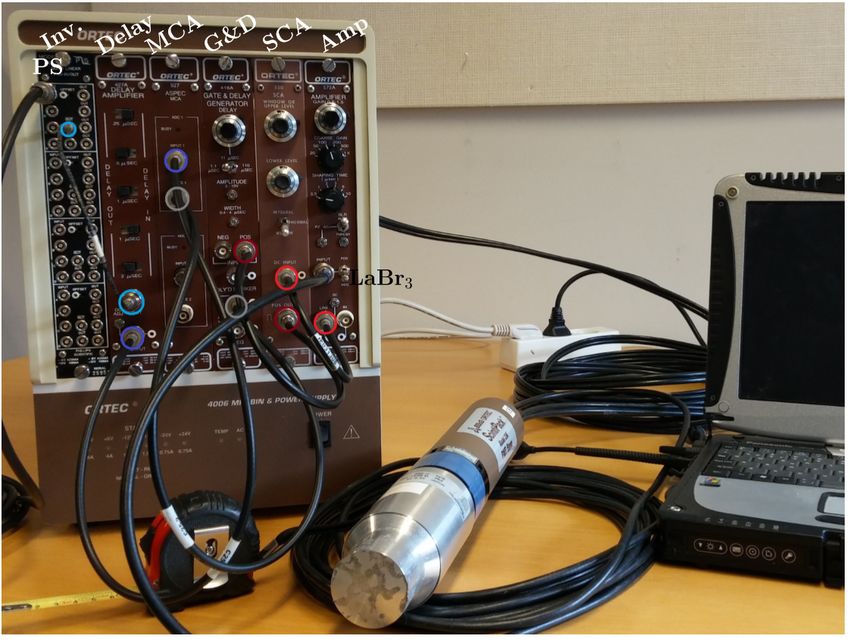
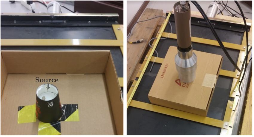
43

  Figure 21. A photograph of a similar PS showing visible defects caused by
  ageing effects. The defects are also within the scintillation material and not
  only at the surface.

5.2.1   Attenuation length: Measurement setup

The setup’s goal is to examine the propagation of scintillation photons along the
PS. For a systematic analysis a constant intensity light source with corresponding
wavelength is required. The solution in this thesis is to investigate a single Compton
scattering energy. Because the number of scintillation photons created per energy
deposited is near to constant, interactions with a fixed energy act as a flickering
photon source within the scintillation material. For other scintillator systems, ex-
amining the photopeaks or simply using a light emitting diode (LED) could be more
convenient. Neither of these methods are possible because the PS only interacts with
the gammas at our energy range of interest via Compton scattering (as shown in
Fig. 1 of Section 2.1), and installing the LED requires disassembling of the PS
casing. In contrast with using an LED, the wavelength of propagating photons are
also naturally at the region of interest when created via scintillation process.
The Compton scattering events chosen for the measurements are the full backscat-
tering events where the initial gamma does a 180◦ scattering from the plastic. In
order to filter out other scintillation events, a secondary scintillator with appropriate
energy resolution is required to detect the backscattered gammas. In our measure-
ment we used two different cylindrical lanthanum bromide (LaBr3 ) crystals (both
Saint-Gobain BrilLanCe 380) with sizes, 1.5"×1.5" and 3"×3" as their length and di-
ameter, respectively. The LaBr3 were mounted onto a PMT base (Ortec ScintiPack,
model 296).
Four sets of measurements were done. First the PS used throughout this thesis was
evaluated in laboratory conditions with both 1.5" and 3" LaBr3 s. Then, two similar
44

operative PSs were evaluated using the 1.5" LaBr3 . In the measurement setup, the
secondary scintillator and the source are positioned as shown in Fig. 22. The on-
field measurement setup is shown in Fig. 23. The distance from the source to PS
was roughly 5 cm and the distance from LaBr3 to the source was roughly 3 cm.
These distances were kept short to minimize the backscattering events that could
occur farther along the PS.

The LaBr3 is now set to detect only the backscattered gammas which have a specific
energy. The events in PS simultaneous with the ones detected in LaBr3 then cor-
respond to the backscattering event itself. This is called as a coincidence method.
In our setup we led the signal from PS through an inverter to an analogue delay
module (Ortec 427A) and fed to the MCA’s input. In the 1.5" lab measurement set
an amplifier (Canberra 2111) with a 10x gain was used in PS signal line to enhance
the channel resolution in MCA. In calculations the channels were scaled back by
dividing the channels by a factor of 10 for comparison purposes. The signal from
LaBr3 is led through an amplifier (Ortec 572A), single channel analyser (SCA, Ortec
550), gate and delay generator (G&D, Ortec 416A) and finally fed to MCA’s gate
input. The SCA module gives out a logical pulse with a width of 500 ns if and
only if the amplitude of the input signal is within a set amplitude window. This
window will be set to match the mentioned backscattering energy. The gate and
delay generator is used to adjust the width of this pulse so that the signal from PS
is within the logic pulse. The delay module in PS signal line is to move the signal
within the said logic pulse. The final signals from an event is shown in Fig. 24.

For field measurements all the modules were mounted on a nuclear instrumentation
module (NIM) rack with an in-built power supply (Ortech Minibin, 4006). The
measurement equipment is shown in Fig. 25.

Both the delay module and amplifier in PS signal line scaled the amplitudes linearly
and didn’t change the pulse width significantly along the whole amplitude range
of interest (not shown here). This is mandatory since the attenuation length is
dependent on the relative amplitudes between different measurements.

The requirement for the radiation source is an easily distinguishable backscattering
peak. In our measurements we used 137 Cs which emits only 661.657 keV gammas
which according to Eq. (1) has a backscattering peak at

                                         661.657 keV
                         E∗ =        661.657 keV
                                1+   510.999 keV
                                                 − cos 180◦ )
                                                 (1
                            = 184.322 . . . ≈ 184 keV.

This is well distinguishable from the backscattering peaks of 40 K and 208 Tl which
are at around 250 keV. Conveniently, the energy is also high enough to penetrate
the radiation monitor casings in our field demonstration.

Coincidence requirement with backscattering peak in LaBr3 means that the energy
You can also read