Diverging land-use projections cause large variability in their impacts on ecosystems and related indicators for ecosystem services - Earth System ...
←
→
Page content transcription
If your browser does not render page correctly, please read the page content below
Earth Syst. Dynam., 12, 327–351, 2021
https://doi.org/10.5194/esd-12-327-2021
© Author(s) 2021. This work is distributed under
the Creative Commons Attribution 4.0 License.

        Diverging land-use projections cause large variability in
        their impacts on ecosystems and related indicators for
                         ecosystem services
       Anita D. Bayer1 , Richard Fuchs1 , Reinhard Mey2 , Andreas Krause3 , Peter H. Verburg4 , Peter Anthoni1 ,
                                                 and Almut Arneth1
          1 Karlsruhe    Institute of Technology (KIT), Institute of Meteorology and Climate Research, Atmospheric
                                Environmental Research, 82467 Garmisch-Partenkirchen, Germany
          2 Swiss Federal Institute for Forest, Snow and Landscape Research WSL, 8903 Birmensdorf, Switzerland
         3 Technical University of Munich, TUM School of Life Sciences Weihenstephan, 85354 Freising, Germany
           4 Institute for Environmental Studies, VU University Amsterdam, 1081HV Amsterdam, the Netherlands

                                  Correspondence: Anita D. Bayer (anita.bayer@kit.edu)

                                     Received: 12 June 2020 – Discussion started: 26 June 2020
                        Revised: 10 February 2021 – Accepted: 14 February 2021 – Published: 30 March 2021

      Abstract. Land-use models and integrated assessment models provide scenarios of land-use and land-cover
      (LULC) changes following pathways or storylines related to different socioeconomic and environmental devel-
      opments. The large diversity of available scenario projections leads to a recognizable variability in impacts on
      land ecosystems and the levels of services provided. We evaluated 16 projections of future LULC until 2040
      that reflected different assumptions regarding socioeconomic demands and modeling protocols. By using these
      LULC projections in a state-of-the-art dynamic global vegetation model, we simulated their effect on selected
      ecosystem service indicators related to ecosystem productivity and carbon sequestration potential, agricultural
      production and the water cycle. We found that although a common trend for agricultural expansion exists across
      the scenarios, where and how particular LULC changes are realized differs widely across models and scenarios.
      They are linked to model-specific considerations of some demands over others and their respective translation
      into LULC changes and also reflect the simplified or missing representation of processes related to land dy-
      namics or other influencing factors (e.g., trade, climate change). As a result, some scenarios show questionable
      and possibly unrealistic features in their LULC allocations, including highly regionalized LULC changes with
      rates of conversion that are contrary to or exceed rates observed in the past. Across the diverging LULC pro-
      jections, we identified positive global trends of net primary productivity (+10.2 % ± 1.4 %), vegetation carbon
      (+9.2 % ± 4.1 %), crop production (+31.2 % ± 12.2 %) and water runoff (+9.3 % ± 1.7 %), and a negative trend
      of soil and litter carbon stocks (−0.5 % ± 0.4 %). The variability in ecosystem service indicators across scenar-
      ios was especially high for vegetation carbon stocks and crop production. Regionally, variability was highest in
      tropical forest regions, especially at current forest boundaries, because of intense and strongly diverging LULC
      change projections in combination with high vegetation productivity dampening or amplifying the effects of cli-
      matic change. Our results emphasize that information on future changes in ecosystem functioning and the related
      ecosystem service indicators should be seen in light of the variability originating from diverging projections of
      LULC. This is necessary to allow for adequate policy support towards sustainable transformations.

Published by Copernicus Publications on behalf of the European Geosciences Union.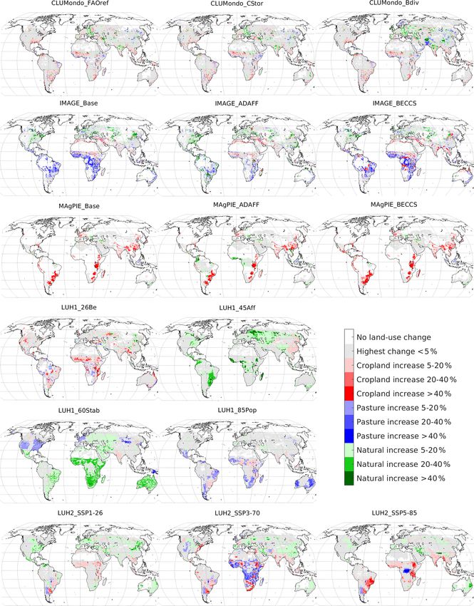
328                 A. D. Bayer et al.: Impact of diverging land-use projections on ecosystems and their service indicators

1   Introduction                                                   identified the differences in projected global LULC associ-
                                                                   ated with the modeling approach to be at least as great as
The recently presented Intergovernmental Panel on Climate          the differences due to scenario variations. In a regional-level
Change (IPCC) Special Report on Climate Change and Land            analysis, Prestele et al. (2016) found the highest uncertainty
(IPCC, 2019) highlighted unprecedented rates of land and           in land-use projections generally at the boundaries of bo-
freshwater use and biodiversity loss and underpinned exist-        real and tropical forests. LULC projections have also been
ing socioeconomic, ecological and climatic challenges such         evaluated in a number of model intercomparison studies, in
as increasing per capita food consumption, land degradation        which models simulated the same scenario storylines based
and an accumulation of climate extreme events. The Inter-          on harmonized drivers, in order to focus on the uncertainty in
governmental Science-Policy Platform on Biodiversity and           LULC changes resulting from structural differences between
Ecosystem Services (IPBES) global assessment report pub-           the models (e.g., Von Lampe et al., 2014; Popp et al., 2017;
lished earlier in 2019 (IPBES, 2019) also reported deteriorat-     Schmitz et al., 2014; Stehfest et al., 2019).
ing levels of most ecosystem services (ESs) and natural cap-          The large uncertainties in LULC projections affect the
ital due to past and current human activities. The cumulative      confidence in projected changes in ecosystem functioning
contribution of land-use and land-cover (LULC) change to           globally, which critically underpins the supply of future ESs
global CO2 emissions has been estimated to about one-third         available to human societies. In the same ways as the effects
of total anthropogenic emissions since preindustrial times         of climate change, the uncertainties arising from different
(Friedlingstein et al., 2019), and total greenhouse gas emis-      LULC projections need to be identified and understood to
sions from LULC in recent years are nearly 25 % of total an-       adapt ecosystems in a sustainable way and possibly coun-
thropogenic emissions (IPCC, 2019). The diversity of current       teract critical regional trends. Studies have focused on the
challenges towards a more sustainable use of land, including       vulnerability of ecosystems and their services to changes in
the maintenance of critical levels of resources and counter-       climate (e.g., Ahlström et al., 2012; Huntingford et al., 2011;
acting climate change, and the various options to approach         Ostberg et al., 2013; Scholze et al., 2006), land use on a
these challenges create a large option space for possible fu-      global or regional scale (e.g., Arora and Boer, 2010; Foley
ture developments of LULC.                                         et al., 2005; Jantz et al., 2015; Krause et al., 2017; Lawler
   Future LULC and changes therein are modeled based on            et al., 2014; Sterling et al., 2013), and a combination of cli-
initial conditions of land use along with LULC history and         mate and land-use effects (e.g., Dunford et al., 2015; Kim
different assumptions about possible socioeconomic and en-         et al., 2018; Krause et al., 2019; Rabin et al., 2020). More-
vironmental developments regarding population growth, in-          over, uncertainties arising from different ES quantification
ternational cooperation, consumption preferences or techno-        methods were estimated (e.g., Schulp et al., 2014). These
logical developments. All of these are represented differently     studies have already begun to document that diverging LULC
in land-use models (LUMs) or integrated assessment models          projections are as important as diverging climate change sce-
(IAMs, e.g., DeFries et al., 2004; Meiyappan et al., 2014; van     narios with respect to the degree of impact on ecosystems.
Vliet et al., 2016). However, these models play a central role        Thus, we expand these previous studies here by bringing
in assessing possible climate change mitigation and adapta-        together a larger number of LULC scenarios and by criti-
tion or conservation strategies in terms of total land demand,     cally examining the resulting variability in diverging LUM
investment and maintenance costs, and direct and indirect so-      projections based on recent historical observations. We in-
cioeconomic and ecological effects (e.g., Humpenöder et al.,       tend to also highlight how different LULC patterns impact
2014; Popp et al., 2014; Reilly et al., 2012).                     ecosystems and related ES indicators. This supports the in-
   In total, the diversity of models, initial model conditions,    terpretation of conclusions derived from LUMs and IAMs
socioeconomic pathways, climate mitigation targets, pro-           towards policy decisions regarding factors such as intensi-
cesses and process feedbacks considered in the LULC mod-           fication, conservation or climate change mitigation options.
eling procedure leads to a large number of diverging land-         A broad range of future LULC projections from different
use projections. This reflects not only the fact that the future   LUMs and different socioeconomic assumptions is impor-
is unknown but also a large uncertainty introduced by the          tant, given the unknown future. Nevertheless, critically as-
model structure itself (e.g., Alexander et al., 2017; Prestele     sessing the spatial pattern and rates of change can support
et al., 2016; Schmitz et al., 2014; Stehfest et al., 2019; van     their interpretation in terms of plausibility.
Vliet et al., 2016). By evaluating a large set of LULC pro-           Our basis was 16 projections of future land use from five
jections (75 and 43, respectively), Alexander et al. (2017)        LUMs or IAMs with different modeling protocols and so-
and Prestele et al. (2016) attributed a significant share of       cioeconomic pathways. Their scenario storylines span a wide
the uncertainty in global and regional LULC projections to         range of world views and policies, with some implemented
the model initial conditions, resulting in part from differ-       to achieve a certain climate mitigation or conservation target
ent LULC definitions (especially for pastures; see also, e.g.,     while others focus only on basic demands for agricultural
Verburg et al., 2011), followed by the model structure, sce-       commodities, built-up area and so on. Models and scenarios
nario storyline and other factors. Alexander et al. (2017)         were assessed based on their underlying demands, modeling

Earth Syst. Dynam., 12, 327–351, 2021                                                https://doi.org/10.5194/esd-12-327-2021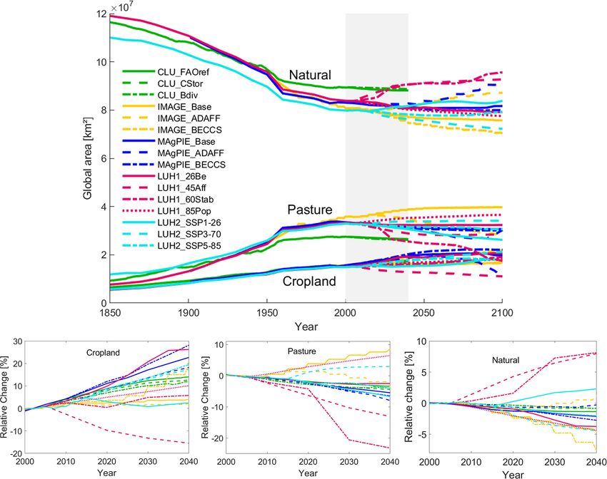
A. D. Bayer et al.: Impact of diverging land-use projections on ecosystems and their service indicators                      329

protocols (e.g., assumptions involved, allocation strategies)     tion growth according to the Shared Socioeconomic Pathway
and the projected spatially explicit land-use futures that they   (SSP) 2 (O’Neill et al., 2014) is available as well as two ad-
describe. We then used the 16 land-use projections as input       ditional scenarios involving land-based climate change mit-
for simulations with a state-of-the-art dynamic global vege-      igation, either via the conservation and expansion of global
tation model (DGVM) to analyze their effects on ecosystem         forest area (ADAFF) or bioenergy crop cultivation and sub-
functionality and six selected ES indicators linked to the pro-   sequent carbon capture and storage (BECCS) (Krause et al.,
ductivity and carbon (C) sequestration potential of ecosys-       2017).
tems (net primary productivity, vegetation C, soil and lit-          MAgPIE is a global land-use model of the agricultural sec-
ter C), agricultural production (crop production) and the wa-     tor (Lotze-Campen et al., 2008; Popp et al., 2014). It opti-
ter cycle (evapotranspiration and annual runoff). We focused      mizes spatially explicit land-use patterns in a recursive dy-
on changes until 2040, i.e., the near to medium future.           namic way to satisfy given commodity demands at minimal
                                                                  production costs while meeting biophysical and socioeco-
                                                                  nomic constraints. Options to fulfill increasing demands are
2     Methods
                                                                  intensification (yield-increasing technologies), cropland and
2.1    Land-use models and scenarios
                                                                  pasture expansion, and international trade. Future land-use
                                                                  projections of the MAgPIE model follow the same storylines
We used a total set of 16 land-use scenarios originating from     as described for IMAGE (Krause et al., 2017).
five different LUMs or IAMs. The models differ in their un-          The Hurtt et al. (2011) modeling approach (LUH1) com-
derlying demands, modeling protocols and technical aspects        bines a historic land-use reconstruction with national statis-
(e.g., number of represented land-use classes, time horizons),    tics of historical wood harvest and assumptions regarding
which are summarized in this section and in Table 1. Al-          shifting cultivation in some tropical regions, and it harmo-
though some of the models considered here are IAMs in-            nizes these data with a set of four future LULC scenarios.
cluding a land-use component, we refer to all models in this      Each scenario was produced by a different IAM with individ-
study as global LUMs for the remainder of this paper because      ual demands and strategies for allocating LULC in response
their projected LULC change is the target of this analysis.       to the demands. The four scenarios follow very different so-
This includes the two versions of the Land-Use Harmoniza-         cioeconomic storylines that are combined with the emissions
tion (LUH) project prominently applied in many studies of         and climate change assumptions of the Representative Con-
the last and the upcoming IPCC reports, although these land-      centration Pathways (RCPs). LUH1 scenarios are not tied to
use products are based on the outputs of several LUMs and         the SSPs, as those were only introduced in 2014. These sce-
IAMs.                                                             narios have frequently been used in the modeling community,
   The CLUMondo model (van Asselen and Verburg, 2013)             especially for the work in the IPCC AR5 (e.g., O’Neill et al.,
applies 30 land system types to model LULC changes. Land          2014; van Vuuren et al., 2014). Here, we used the version of
systems define typical combinations of shares of cropland,        LUH1 which had the historical dataset extended until 2014
grassland, bare land and built-up land as well as a specific      (Le Quéré et al., 2015) as well as future trajectories following
management intensity (e.g., extensive cropland with few live-     IAM implementations of RCPs 2.6, 4.5, 6.0 and 8.5.
stock). Land systems are dynamically allocated based on lo-          The Land-Use Harmonization v2 (LUH2; v2.1, Hurtt
cal suitability, spatial restrictions and the competition be-     et al., 2020) has been developed for the Coupled Model In-
tween land systems to fulfill demands that were created ex-       tercomparison Project Phase 6 (CMIP6; Eyring et al., 2016).
ogenously by the IMAGE model on the level of world re-            It follows a similar methodology as in LUH1, although on
gions. Trade between world regions is excluded in CLU-            a higher spatial resolution and over a longer time domain,
Mondo. Eitelberg et al. (2016) designed three CLUMondo            using updated historical land-use reconstructions along with
scenarios: a reference scenario following the development         updated models of past and future land transitions and man-
of basic demands as expected by the Food and Agriculture          agement (e.g., wood harvest, crop rotations and shifting cul-
Organization (FAO) and two scenarios that additionally in-        tivation) and extending the number of scenarios by combin-
cluded a policy target of reducing deforestation and green-       ing RCPs with SSPs. Similar to LUH1, future LULC transi-
house gas emissions with a higher ecosystem carbon storage        tions in LUH2 are based on land-use projections from differ-
and international policy targets for the prevention of biodi-     ent IAMs that each follow their own strategy for allocating
versity loss.                                                     LULC in response to demands. Of the eight scenarios that
   The Integrated Model to Assess the Global Environment          have been harmonized in LUH2 with historical data, three
(IMAGE) is an IAM framework including sub-models rep-             scenarios were selected (SSP1-26, SSP3-70 and SSP5-85)
resenting the energy system, agricultural economy, land use       to span the range from low to high radiative forcing as in
and the climate system (Stehfest et al., 2014). LULC alloca-      the LUH1 scenarios in combination with diverging land-use
tion is done following an assessment and ranking of land’s        trends according to the SSPs.
suitability to fulfill demands. From IMAGE, a LULC base-
line projection following increased food demand and popula-

https://doi.org/10.5194/esd-12-327-2021                                              Earth Syst. Dynam., 12, 327–351, 2021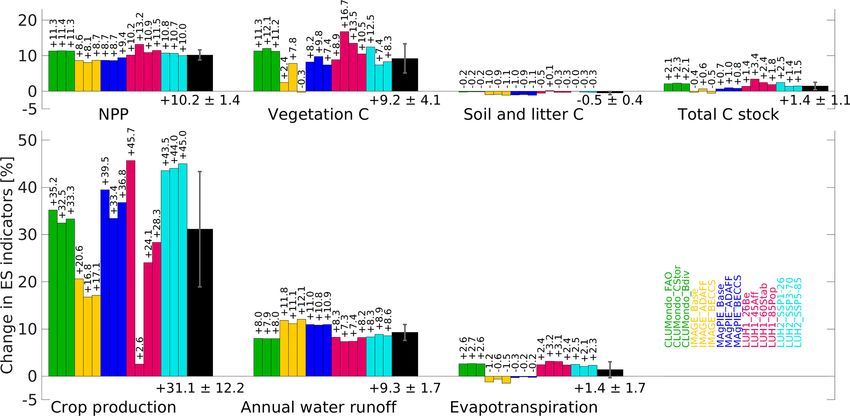
A. D. Bayer et al.: Impact of diverging land-use projections on ecosystems and their service indicators
https://doi.org/10.5194/esd-12-327-2021
Table 1. Overview of land-use models and scenarios used in this study. Main references are given for each model and the scenarios applied in this study; the reader is also referred to
the references therein for further details.
Land-use model Technical characteristics1 LU categories and additional information Allocation procedure Consideration of climate change
CLUMondo S: 9.25 km × 9.25 km, Eckert IV pro- A total of 24 land system types as combi- Spatially explicit allocation of land systems to fulfill the demand of 24 world None; present climate and
(van Asselen and jection; nations of extensive, medium intensive, or regions. As long as demands are not satisfied, land systems that contribute more atmospheric CO2 level are as-
Verburg, 2013; T: future 2001–2040, annual; intensive cropland, mosaic cropland, and to a standing demand are preferred. No trade between world regions is assumed. sumed.
Eitelberg et al., B: starts from land use in 2000 fol- grassland, dense or open forest, bare land
2016) lowing Ramankutty et al. (2008). and built-up area (note that pigs and poul-
try are excluded as a defining characteris-
tic).
IMAGE S: 26 world regions (for socioeco- Fractional data for cropland, pasture, for- Allocation relies on regression-based suitability assessment and iterative allo- Yes; all scenarios are based
(Popp et al., 2017; nomic parameters), est, urban and other natural land. cation procedure until demands are met. on RCP2.6 climate from
Stehfest et al., 0.5◦ × 0.5◦ (most environmental pa- the IPSLCM5A-LR general
2014) rameters, including land use); circulation model bias corrected
T: historic 1970–2005, future 2005– to the 1960–1999 historical
2100, annual; period. Varying CO2 level with
B: LU harmonized to HYDE 3.1 490 ppm in 2100.
(Klein Goldewijk et al., 2011) in
20052 .
MAgPIE S: 10 world regions, (0.5◦ × 0.5◦ res- Fractional data for cropland (irrigated, Achieve demands under minimizing costs in 10 world regions with recursive Yes; all scenarios are based on
(Lotze-Campen olution, clustered to 500 units based nonirrigated), dynamic optimization. Cost minimization defines land availability. International RCP2.6 climate impacts – same
et al., 2008; Popp on “similarity” in the modeling; see pasture, forest, urban and other natural trade considered (Humpenöder et al., 2014). as IMAGE.
et al., 2014, 2017) Humpenöder et al., 2014); lands.
T: future 1995–2100, 5-year steps;
B: LU harmonized to HYDE 3.1
(Klein Goldewijk et al., 2011) in
1995.
LUH1 S: 0.5◦ × 0.5◦ , WGS84; Fractional data for cropland, pasture, pri- Allocation for historic period based on HYDE 3.1 (land use/capita using weigh- Yes; consideration of
(Hurtt et al., 2011) T: historic 1500–2005, future 2005– mary vegetation, secondary vegetation and ing maps for built-up areas, population density, soil suitability, coastal ar- different Representative
2100, annual; urban; gross transitions between land-use eas/river plains, annual mean temperature). Concentration Pathways (RCPs)
B: historic product is based on Klein classes based on shifting cultivation in Additionally, LUH1 uses the following features to process land-use change: from the different IAMs.
Goldewijk et al. (2011). some tropical regions. – shifting cultivation rates;
– deforestation for agricultural land included in wood harvest statistics;
Earth Syst. Dynam., 12, 327–351, 2021
– priority for land conversion (agricultural land taken from primary or sec-
ondary).
For the future, the allocation is dependent on the four IAMs used for the sce-
narios (at a 2◦ × 2◦ resolution), disaggregated to 0.5◦ × 0.5◦ .
LUH2 S. 0.25◦ × 0.25◦ , WGS84; Fractions for cropland (C3 /C4 annuals, Allocation for the historic period is based on HYDE 3.2 and globally available Yes; consideration of different
(Hurtt et al., 2020; T: historic 850–2015, future 2016– C3 /C4 perennials, C3 nitrogen fixing), statistics and for the future period based on transitions and additional informa- RCPs from the different IAMs.
data from 2100, annual; managed pasture, rangeland, primary land, tion from IAMs (see also their respective allocation procedures; compare refer-
http://luh.umd.edu, B: 850–2015 land use based on secondary land and urban areas. ences in Hurtt et al., 2020).
last access: 1 June HYDE 3.2 (Goldewijk et al., 2017). Additionally, LUH2 uses the following features to process land-use change:
2019) – crop type and rotations;
– shifting cultivation rates;
– historical wood harvest statistics and future forest transitions;
– biomass density and recovery rates;
– priority for land conversion.
330Table 1. Continued.
Scenarios
– FAOref: demands with respect to tons of crop production, size of livestock and population (as built-up area) as expected by the FAO until 2040. Demands projected to 24 world regions by the integrated
assessment model IMAGE.
– CStor: in addition to FAOref there is extra demand for C storage implemented with a no-carbon-loss approach. This results in the favorable consideration of land systems with high C storage capacity such as
dense forests in the allocation procedure.
– Bdiv: in addition to FAOref there is extra demand for protected areas. Protected areas are used that follow national biodiversity targets according to Aichi Target 11. Forest and grassland proportions were
selected to account for protected areas in the CLUMondo land systems “dense forest”, “mosaic grassland and forest”, “mosaic grassland and bare” and “natural grassland”. Favorable consideration of land
systems with high amount of protected areas in the allocation procedure. Land systems in land areas assigned to the International Union for Conservation of Nature (IUCN) categories I to IV at the beginning
of the simulation procedure were maintained throughout the scenario.
– Base: land-use change is driven by increased food demand and population growth according to SSP2.
– ADAFF: demands are the same as in the Base scenario with an additional CDR target of 130 Gt C by 2100. Land-based mitigation achieved by avoiding deforestation and afforestation.
https://doi.org/10.5194/esd-12-327-2021
– BECCS: demands are the same as in the Base scenario with an additional CDR target of 130 Gt C by 2100. Land-based mitigation is achieved by bioenergy plant cultivation and subsequent carbon capture
and storage.
– Base: land-use change is driven by increased food demand and population growth according to SSP2.
– ADAFF: demands are the same as in the Base scenario with an additional CDR target of 130 Gt C by 2100. Land-based mitigation is achieved by avoiding deforestation and afforestation.
– BECCS: demands are the same as in the Base scenario with an additional CDR target of 130 Gt C by 2100. Land-based mitigation is achieved by bioenergy plant cultivation and subsequent carbon capture
and storage.
– 26Be: scenario following RCP2.6 where the cultivation of bioenergy crops with CCS sequestering carbon significantly balances C so that global warming saturates below 2 ◦ C until 2100. There is increased
land demand for bioenergy crops, which occur near existing agricultural areas, and natural areas are declining. Simulated by IMAGE IAM.
– 45Aff: scenario following RCP4.5 assuming that global greenhouse gas emission prices support climate change mitigation by massive afforestation programs around the world with the aim of preserving
large C stocks in forests. Vast expansion of forested area slightly decreases the area of arable land, but assumed technological improvements and more efficient global trading systems maintain agricultural
production to satisfy demands. Simulated by the dynamic recursive economic model GCAM.
– 60Stab: scenario following RCP6.0 assuming stabilization with a medium population growth throughout the 21st century; climate change mitigation efforts only become effective in the last third of the
century. Intensification and expansion of cropland area cover the increased food demand. Simulated by AIM and other models.
– 85Pop: scenario following RCP8.5 assuming rapid population growth to 12 billion people in 2100 and a global temperature rise of more than 4 ◦ C by 2100. Intensification is supported by technological
improvements as the most important driving factor to satisfy a high food demand. Cropland expands as well as pasture, especially in developing countries, while natural areas decline. Simulated by
MESSAGE IAM.
– SSP1-26: scenario combining SSP1 and RCP2.6 of an environmentally friendly world with low population growth, high urbanization, relatively low demand for animal products and high agricultural
productivity. Land use and land-use change is relatively low, and policies targeting the reduction of atmospheric greenhouse gases (including BECCS and afforestation) are implemented so that an additional
forcing is limited to 2.6 W m−2 by 2100. Simulated by IMAGE 3.0 IAM, where LULC is allocated iteratively based on suitability assessment until demands are met.
A. D. Bayer et al.: Impact of diverging land-use projections on ecosystems and their service indicators
– SSP3-70: scenario combining SSP3 and RCP7.0 that is focused on regional development. High population growth in developing countries as well as slow economic development and per capita food
consumption lead to the high expansion of agricultural areas rather than agricultural land intensification under a relatively high level of climate change with a radiative forcing of 7.0 W m−2 by 2100.
Simulated by the AIM/GCE IAM framework and based on the adjustment of prices until supply and demand for commodities and services equilibrate.
– SSP5-85: scenario combining SSP5 and RCP8.5 of a world characterized by strong economic growth that is based on fossil fuels, with low population growth, high urbanization, and high food demand per
capita with high agricultural productivity due to technological progress. Strong expansion of global cropland and the level of climate change is high with an assumed radiative forcing of 8.5 W m−2 by 2100.
Simulated by the REMIND/MAgPIE IAM framework, where LULC changes are modeled chiefly based on prices and quantities of bioenergy and greenhouse gas emissions.
1 “S” represents spatial resolution and projection, “T” represents time horizons, and “B” represents underlying databases or the historical land-use baseline from which scenarios start. 2 Small deviations in the area of the land-cover classes between IMAGE/MAgPIE and HYDE
Earth Syst. Dynam., 12, 327–351, 2021
331
3.1 land use in 1995/2005 occur due to different land masks and calibration routines.332 A. D. Bayer et al.: Impact of diverging land-use projections on ecosystems and their service indicators
2.2 LPJ-GUESS model dle of an ensemble of a wider range of GCMs used in the
Inter-Sectoral Impact Model Intercomparison Project (ISI-
The process-based dynamic global vegetation model LPJ- MIP; Warszawski et al., 2014). Climate projections and CO2
GUESS simulates vegetation dynamics in response to cli- concentrations followed the RCP2.6 pathway. Large mag-
mate, atmospheric CO2 , land-use change (Lindeskog et al., nitudes of climate change and high atmospheric CO2 con-
2013) and nitrogen (N) dynamics (Olin et al., 2015; Smith centrations affect ES indicators notably (see, e.g., Alexander
et al., 2014). Three distinct land-use types are represented et al., 2018). As our focus here is on the impact of land-use
(natural vegetation, pasture and cropland). Vegetation dy- change, we chose a climate change projection that would
namics in natural areas are characterized by the establish- have relatively little additional impact over the simulation
ment, competition and mortality of 12 plant functional types period. In a sensitivity experiment, we explore the range of
(PFTs, 10 woody and C3 and C4 grass types, as in Smith variability due to different climate models using the RCP2.6
et al., 2014), which are distinguished in terms of their bio- outputs from the GFDL-ESM2M, HadGEM2-ES, MIROC-
climatic preferences, photosynthetic pathways and growth ESM-CHEM and NorESM1-M models (Warszawski et al.,
strategies. Pastures are populated with competing C3 and 2014) and LULC from the four LUH1 scenarios.
C4 grass PFTs, where 50 % of the aboveground biomass is We modeled the ice-free land surface and included only
removed each year as a representation of grazing (Lindeskog those grid cells in our simulations for which all LUMs pro-
et al., 2013). Croplands are represented by prescribed frac- vided data. Table S1 in the Supplement provides the de-
tions of crop functional types (CFTs, i.e., C3 crops with tailed simulation setup with all forcing data for the LPJ-
winter and spring sowing dates, C4 crops and rice), with GUESS simulations. The differences in the modeling proto-
crop-specific processes including dedicated carbon alloca- col of CLUMondo/LUH1/LUH2 and IMAGE/MAgPIE sim-
tion and phenology, explicit sowing and harvest represen- ulations will affect the base level of ES indicators in 2000–
tation, irrigation, fertilization and unmanaged cover grass 2004 to some degree, although the impacts of slightly diverg-
growing between cropping seasons (Olin et al., 2015). Crops ing historical model periods, spin-up and historical climate
are prescribed to be either rain-fed or irrigated (Lindeskog would have mostly disappeared by the beginning of the 21st
et al., 2013). LPJ-GUESS does not assume yield increases century (baseline period). Larger effects arise from the intrin-
due to technological progress (such as advanced new vari- sic differences in the individual LUMs (see also Alexander
eties, management techniques, pest control), but yields re- et al., 2017). In principle, differences in the baseline land-
spond to changes in climate, atmospheric CO2 concentra- cover maps could spill over to the simulated degree of change
tion, N input (deposition and fertilizer rates) and the frac- in the future scenarios. For instance, the presence or absence
tion of rain-fed vs. irrigated cropland. Adaptation to climate of natural vegetation in the baseline maps might translate
change is partially accounted for by a dynamic calculation of into variable degrees of future (semi)natural vegetation re-
potential heat units (PHU) needed for the full development growth. However, this would only be an important consid-
of a crop before harvest, simulating the adequate selection eration when comparing similar scenarios (and their under-
of suitable crop varieties under changing climate (see Lin- pinning storylines related to factors such as sustainability).
deskog et al., 2013). Upon conversion of forested natural land The alternative approach of harmonizing the different pro-
for agriculture, 20 % of the woody biomass enters a prod- jections to the same starting point of land cover would ar-
uct pool (turnover time of 25 years), with the rest being di- tificially mask some of the simulated differences in ES in-
rectly oxidized (74 %) or decomposed as litter (6 %). Follow- dicators which would be contrary to our objectives. There-
ing agricultural abandonment, natural vegetation recolonizes fore, LUM data were taken as they are, with each LUM sce-
the land in a typical succession from herbaceous to woody nario providing a seamless transition from historical to fu-
plants, with competition for resources and light among age ture, which is needed to simulate vegetation and carbon cycle
cohorts of woody PFTs simulated directly through forest gap responses.
dynamics. In natural ecosystems, fire is simulated explicitly Some of the variables assessed in LPJ-GUESS would also
as a recurring disturbance, while other episodic events (such be computed in the models that deliver the LULC change
as insect outbreaks or windthrow) are subsumed in a back- scenarios – most notably crop yields and some carbon-cycle-
ground disturbance that occurs with a probability of 1 % each or water-cycle-related variables. The spatial patterns of these
year. would differ in the LUMs and LPJ-GUESS. However, this
does not affect our analysis: here we take the LULC change
2.3 Simulation setup projections in a unidirectional approach to assess impacts on
ecosystem processes; we do not compare similar ecosystem
LPJ-GUESS was run at a 0.5◦ × 0.5◦ resolution and forced output variables across different model types.
by the monthly climate of the IPSL-CM5A-LR general cir- LULC fractions were taken as net annual transitions from
culation model (GCM). The model projects a global aver- the LUMs and aggregated to the three land-use types – crop-
age surface temperature increase of about 1.3 ◦ C by the end land, pasture and natural land – used by LPJ-GUESS (see
of the century relative to 1980–2009, which lies in the mid- Table S2 in the Supplement) and to the spatial resolution
Earth Syst. Dynam., 12, 327–351, 2021 https://doi.org/10.5194/esd-12-327-2021A. D. Bayer et al.: Impact of diverging land-use projections on ecosystems and their service indicators 333
of 0.5◦ × 0.5◦ if needed. Cropland fractions also included tially takes account of differences in baseline LULC patterns
bioenergy areas, and pasture fractions included degraded and ES provision levels across the scenarios.
forests (IMAGE only), rangeland and grazing land. As LPJ-
GUESS does not represent urban land, built-up areas were
3 Results
included in the natural land fraction. Where 0.5◦ grid cells
contain substantial shares of water, this fraction was assigned 3.1 Strategies of LUMs to translate demands into
to bare land, i.e., excluded from the simulation of vegetation land-use changes
pattern in LPJ-GUESS. In CLUMondo, LULC changes do
not occur between land-cover types but between more com- Figures 1 and 2 summarize LULC changes in the 16 pro-
plex land-use systems (see Sect. 2.1) that have different com- jections. The scenarios projected total changes in LULC of
positions in terms of natural, pasture and cropland area. In about 4.5 % to 11.4 % of the global ice-free land surface from
addition, the fractions of each land system vary regionally. 2000 to 2040 (Table 2), corresponding to different transi-
In our simulations, we did not include wood harvest. In the tions between crop, pasture and natural land. While differ-
BECCS scenarios we assumed 80 % of the harvested C from ent socioeconomic assumptions realized as land-use change
bioenergy crops to be captured and stored following Krause projections by the same model led only to small variations
et al. (2017). in the outcomes in terms of absolute rates (see Fig. 1, Ta-
ble 2) and spatial patterns of LULC changes (see Fig. 2),
the variation in LULC change between models was much
2.4 Simulation of ecosystem service indicators more important, including for similar socioeconomic scenar-
ios. This highlights the importance of the differences in mod-
Changes in ecosystem function and services were assessed eling strategies. In this regard, we realize that the outcomes
using a suite of regulating and provisioning ES indicators: net as described are indicative of the models’ behaviors for the
primary productivity (NPP, foremost an indicator for ecosys- particular scenarios considered in this study, which are not
tem productivity and C sequestration related to global cli- necessarily but very likely representative of the models’ gen-
mate regulation, also used as indicator for ecosystem health), eral behaviors upon projecting future LULC patterns. LUH1
C storage (natural capital that underpins and is closely re- and 2 are exceptions with regard to the changes in between
lated to C sequestration and global climate regulation), crop scenarios, because individual scenario data originate from
production (contributing to food supply), annual water runoff different LUMs; therefore, their data differ substantially be-
(indicator for water availability but also related to flood regu- tween all scenarios.
lation) and evapotranspiration (indicator for regional climate In comparison to the other LUMs, CLUMondo shows
regulation). C storage was investigated for vegetation, soil rather small-scale LULC changes spread across large parts
and litter C as well as total C, with the latter also includ- of the world (Fig. 2). The three scenarios have the same de-
ing carbon stored via carbon capture and storage (CCS) in mands for livestock, crop production, and so on, and the addi-
BECCS scenarios. All plant and crop functional types con- tional objectives in terms of C uptake and storage or biodiver-
tribute to an ecosystems’ NPP. Therefore, NPP and crop sity conservation did not introduce large variations. There-
production are positively correlated. All variables are di- fore, differences between the CLUMondo scenarios are small
rect outputs of LPJ-GUESS simulations. Baseline crop yields (see Table 2). The biodiversity scenario leads to the most land
of each run were scaled to FAO observed yields in 1997– area changes due to land system classes that diverge to either
2003 as in Krause et al. (2017). Yields respond to changes system intensification in some regions or extensification in
in climate and CO2 , also including some degree of adapta- others. Demands are fulfilled by almost linear trends until
tion, which arises from the calculation of dynamic PHU (see 2040 based on the assumed scenario storyline and demand
Sect. 2.2). Adaptation related to factors such as choosing dif- estimates (Fig. 1).
ferent crop species in a grid cell was not considered here in Land-use changes in the three IMAGE scenarios also af-
simulations of the future period. Changes in ES indicators fect most of the productive land areas globally. Compared
were analyzed for each LULC scenario as percent change with CLUMondo, spatial patterns are different and the spread
in 2036–2040 relative to the base level in 2000–2004. The of percentage area changes across scenarios is higher (glob-
average of 5 years was used to reduce the influence of in- ally 5 %–10 % difference per LULC class for IMAGE sce-
terannual variability. As climatic and atmospheric changes narios; Table 2). Global trends are not linear; some scenar-
are identical across the simulations, differences in ES indica- ios even reverse their historic trend (e.g., IMAGE_ADAFF
tor changes across the scenarios mostly reflect the immediate scenario for pasture) or accelerate it (e.g., IMAGE_BECCS
and long-term effects of changes in LULC, also considering scenario for cropland), possibly driven by the introduction
that climate change impacts might be dampened or amplified of new land-use policies. In IMAGE, food production meet-
depending on the vegetation cover existing in a grid location. ing the underlying societal demand has large priority. The
The evaluation of percent changes in future LULC and ES IMAGE_Base scenario accordingly increases pasture area
indicators relative to the baseline period in 2000–2004 par- at the cost of natural land (presumably to satisfy demand
https://doi.org/10.5194/esd-12-327-2021 Earth Syst. Dynam., 12, 327–351, 2021334 A. D. Bayer et al.: Impact of diverging land-use projections on ecosystems and their service indicators Figure 1. Absolute land area of croplands, pastures and natural areas between 1850 and 2100 for 16 scenarios of five land-use models, and the detailed relative changes in LU from 2000 to 2040 analyzed in this study. for animal products in the underlying “SSP2” world) while strongly depend on minimizing the costs of land conversion. cropland increases only slightly, presumably because yield Here, some countries seem to provide substantially cheaper increases satisfy the increasing food demand of a growing commodity prices than others, explaining the radical changes population. The afforestation and reforestation scenario IM- seen in the regions as listed above (compare also Fig. 2). AGE_ADAFF partially reverses IMAGE_Base by expand- It is noteworthy that MAgPIE and IMAGE derive potential ing natural land at the cost of pasture land, whereas IM- crop yields and ecosystem C densities from the same DGVM AGE_BECCS, in addition to pasture expansion as in IM- (LPJmL, Bondeau et al., 2007), even though internal yield AGE_Base, also expands cropland areas at the cost of natu- scaling and forest growth curves are implemented differently. ral land. Spatially, the distribution of land-use classes among However, their spatial patterns are quite different, emphasiz- all scenarios differs little, indicating that demands from the ing the role of individual strategies to translate demands un- IMAGE_Base scenario (e.g., population growth, diets, food der similar biophysical constraints into LULC patterns. Fur- demand, trade) outweigh specific scenario demands. thermore, the land demand to meet the same carbon dioxide In MAgPIE, land changes only occur in specific regions removal (CDR) target was found to be larger in IMAGE than or countries, although the changes in these regions are mas- in MAgPIE (Krause et al., 2018). sive (southeastern Argentina and southern Brazil, some coun- In contrast, land changes in all LUH1 scenarios are large tries in eastern Africa, and parts of southern and eastern and occur in most of the productive land areas globally, re- Asia), with the dominant change by far being cropland ex- flecting both the highly diverging socioeconomic storylines pansion. The three MAgPIE scenarios differ relatively little as well as their implementation by different IAMs (see Ta- in time and space: only the afforestation and reforestation ble 2). Trends over time are nonlinear but involve multiple scenario again shows some very local natural area expan- break points or gradual slopes. Interestingly, LUH1_26Be, sion. Trends over time are linear. Decisions regarding where which was developed by the IMAGE model (Hurtt et al., land-use change takes place to meet food and feed demand 2011), focuses on a broad expansion of croplands in tropical Earth Syst. Dynam., 12, 327–351, 2021 https://doi.org/10.5194/esd-12-327-2021
A. D. Bayer et al.: Impact of diverging land-use projections on ecosystems and their service indicators                           335

Figure 2. Categories of dominant land-use change from 2000–2004 to 2036–2040 for each of 16 land-use scenarios. The legend is identical
for all plots.

regions, whereas IMAGE_BECCS (although most likely im-                even more so LUH1_60Stab focus on the massive expansion
plementing a different degree of bioenergy growth) includes           of natural areas in all global regions where forests can be sus-
a massive relocation of pastures and croplands to tropical            tained, whereas LUH1_85Pop expands pastures and secon-
and subtropical areas, respectively (Fig. 2). LUH1_45Aff and          darily croplands in tropical and subtropical areas. The attri-

https://doi.org/10.5194/esd-12-327-2021                                                   Earth Syst. Dynam., 12, 327–351, 2021
336                  A. D. Bayer et al.: Impact of diverging land-use projections on ecosystems and their service indicators

Table 2. Total area of cropland, pasture and natural land as well as the change therein from 2000–2004 to 2036–2040 for 16 land-use
scenarios. For each scenario, the left column gives the global total area for 2000–2004 (upper value) and 2036–2040 (lower value) and the
right column gives the change from 2000–2004 to 2036–2040 in absolute terms (upper value) and as a percentage relative to the level in
2000–2004 (lower value). Gray shading indicates a positive or negative trend. Total area under change from 2000 to 2040 is given in absolute
terms and as a percentage of the global ice-free land area considered in this study (see Sect. 2). Minor deviations in numbers may occur due
to rounding.

bution of specific spatial LULC patterns to model allocation            also in Australia, some cropland expansion and a reduction in
strategies vs. scenario storylines is impossible for LUH1, and          pastures (Figs. 1 and 2). LUH2_SSP3-70, in contrast, results
in the same way also for LUH2, because underlying IAMs                  in a massive cropland expansion in some regions, in com-
and storylines differ between each scenario.                            bination with a relocation of pastures, while LUH2_SSP5-
   LUH2 scenarios also differ substantially, corresponding to           85 (implemented by REMIND/MAgPIE) shows very large
the very different SSP storylines and RCPs combined with                and concentrated regional dynamics, with cropland expan-
their origin from different IAMs. LUH2’s SSP1-26 (also im-              sion similar to the MAgPIE scenarios as presented above.
plemented by IMAGE but with different socioeconomic as-                    In summary, most scenarios only agreed on a trend for
sumptions than IMAGE_BECCS and LUH1_26Be), which                        cropland expansion at the cost of natural or pasture areas
includes options for both bioenergy crops and forest re-                in terms of total area (see also Fig. 1). Moreover, the sce-
growth, shows expansion of natural areas mostly in temper-              narios showed very diverse patterns with respect to where
ate (and some boreal) regions of the northern latitudes and             and how these changes were realized. Thus, the deviation in

Earth Syst. Dynam., 12, 327–351, 2021                                                       https://doi.org/10.5194/esd-12-327-2021
A. D. Bayer et al.: Impact of diverging land-use projections on ecosystems and their service indicators                        337

LULC changes from 2000–2004 to 2036–2040 across the                 that these studies applied different LULC data and used LPJ-
scenarios (Fig. S1 in the Supplement) showed major dis-             GUESS without C–N limitation and with differing model se-
agreement for cropland, pasture and natural areas. Standard         tups. Regionally, increases in vegetation productivity and C
deviations of changes in land area > 20 % across all scenar-        stocks were pronounced in boreal and temperate forests. In
ios were found for all three LULC classes over wide world           the tropics, the positive effects of factors such as CO2 fertil-
regions, especially in southeastern South America, the entire       ization and improved water use efficiency (see, e.g., Wårlind
sub-Saharan and eastern African region, and some regions            et al., 2014) were partially offset by cropland and pasture ex-
in Europe and southern Asia. This partially agreed with fea-        pansion, together with the negative effects of a warmer and
tures that were identified in earlier studies evaluating a set of   drier climate. Across the 16 scenarios, the increase in NPP
multiple model LULC projections, such as in terms of global         and C storage was generally higher in CLUMondo, LUH1
and regional trends (Schmitz et al., 2014) and the location of      and LUH2 than in the IMAGE and MAgPIE scenarios. In-
hotspots of uncertainty in LULC projections (Prestele et al.,       creases in vegetation and total C stocks were, as expected,
2016). Given the diversity in socioeconomic storylines and          large in scenarios that showed significant amounts of for-
LUMs, these findings are not surprising, but they highlight         est regrowth (especially LUH1_45Aff, LUH1_60Stab and
(1) the need to critically reflect on which of the observed         LUH2_SSP1-26 but also IMAGE/MAgPIE_ADAFF) and
LULC change patterns might be considered more or less re-           low in scenarios with agricultural expansion for food (e.g.,
alistic given historical regional developments in combination       IMAGE_Base and LUH1_85Pop) or bioenergy production
with environmental, economic and political constraints such         (IMAGE/MAgPIE_BECCS and LUH1_26Be). The overall
as water availability, yield gaps and governance issues (see        changes in total C stocks reflected an increase in vegeta-
Sect. 4.1), and (2) the need to explore the existing uncer-         tion C (+9.2 % ± 4.1 %) that was balanced to some degree
tainty in terms of future LULC regarding the implications           by a decrease in soil and litter C stocks (−0.5 % ± 0.4 %),
for ES indicators beyond yields (see Sect. 4.2).                    likely driven by enhanced respiration of organic material un-
                                                                    der warmer temperatures (see, e.g., Pugh et al., 2015), in
3.2   ES indicators for alternative LULC scenarios
                                                                    combination with the negative effects of decreasing natural
                                                                    areas on soil and litter C in most scenarios. The simulated
The 16 land-use scenarios resulted in very diverse levels of        increase in vegetation C was significantly lower and the de-
ES indicators in 2000–2004 and changes therein until 2036–          crease in soil and litter C was larger for all IMAGE and MAg-
2040 simulated with LPJ-GUESS (see Fig. 3 and Table S3              PIE scenarios because the conversion of natural land to pas-
in the Supplement for all results given in the following). Fig-     tures (for IMAGE) and to croplands (for MAgPIE) in these
ure 4 shows the spatial distribution of categories in ES in-        scenarios was largest among the different scenarios analyzed
dicator levels and their changes until 2036–2040, averaged          in this work.
across the 16 scenarios. We decided to also investigate av-            Crop production was simulated to increase on average
erages in order to explore some overall emerging trends in          across all 16 scenarios by 31.2 % ± 12.2 %; this was partly as
ES indicators that result from the combined effects of cli-         a result of total cropland area increasing (+11.7 % ± 10.5 %,
mate and land-use change on ecosystem functionality. The            Tables 2 and S3) for all scenarios except for LUH1_45Aff
average maps are complemented by the regional variability           and partly due to increasing yields. Yield increases resulted
in ES indicators (right column in Fig. 4, see also Sect. 4.2)       from the joint effects of increased N fertilization rates,
as a measure of the large between-scenario variability in ES        warmer temperatures in some regions and increasing atmo-
indicators. Where regional variability is low, differences in       spheric CO2 (see Fig. S4 in Krause et al., 2017). Crop pro-
LULC across scenarios are small and ES indicator changes            duction increases were found in all world regions, espe-
can solely be attributed to climatic changes and/or changing        cially southern and eastern Asia, central and southern Africa,
CO2 concentration along with the joint trend in LULC shown          southeastern South America, and cropping regions in North
by all scenarios for this location.                                 America and Europe. Differences in crop production be-
   The declining trend in natural areas (average decline            tween scenarios were due to different absolute area and the
of 0.9 % ± 4.0 % by 2036–2040 across 16 scenarios) as               location of cropland expansion on the globe (and differences
shown by most LUMs (Table 2) is balanced by the com-                in N fertilization rates for IMAGE and MAgPIE scenar-
bined positive effect of increased atmospheric CO2 con-             ios, see Sect. 2). For LUH1_45Aff, the simulated global to-
centrations, N deposition and warmer climate (especially at         tal increase in crop production was only 2.6 % because of
higher latitudes), leading to an increased global vegetation        the immense amount of natural area expansion in this sce-
productivity (+10.2 % ± 1.4 %) and higher total C stocks            nario reducing total cropland area in contrast to the other
(+1.4 % ± 1.1 %) overall across the scenarios. Simulated            15 scenarios. Furthermore, LUH1_60Stab and all IMAGE
changes agreed with respect to the trend but levels were be-        scenarios showed lower increases in crop production than
low those reported in previous studies (compare LPJ-GUESS           the other scenarios due to only small cropland expansion
simulations including LULC changes for the IPSL-CM5A-               (for LUH1_60Stab) and newly established croplands being
LR climate of Brovkin et al., 2013; Pugh et al., 2018), noting      chiefly located in low- to medium-production areas (for the

https://doi.org/10.5194/esd-12-327-2021                                                Earth Syst. Dynam., 12, 327–351, 2021
338 A. D. Bayer et al.: Impact of diverging land-use projections on ecosystems and their service indicators Figure 3. Change and uncertainty in ES indicators from 2000–2004 to 2036–2040 as a percentage relative to the base level in 2000–2004 across 16 land-use scenarios. Black bars give the average and standard deviation of the relative changes across all scenarios. See Table S3 for absolute levels and changes for each scenario. IMAGE scenarios, e.g., sub-Saharan and northern Africa and et al., 2017; Rabin et al., 2020). Increases in runoff were sim- the Middle East). For all LUH2 scenarios, crop production ulated in the temperate zone and higher northern latitudes increases were high – about 44 % relative to the level in and in smaller regions in the tropical and subtropical zone. 2000–2004. Lower crop production was simulated in IM- In water-limited regions such as the subtropics, some of this AGE and MAgPIE climate change mitigation scenarios com- water could, in principle, be available for irrigation, depend- pared with their baseline scenarios and also in CLUMondo ing greatly on the regional annual runoff dynamics. However, scenarios when additional land demands had to be met com- it will also increase erosion of soil and nutrients (e.g., Sal- pared with their FAO reference scenario. This highlights the vati et al., 2014) and the risk for floods in some regions (see, inherent trade-off created through multiple demands. It has e.g., Rabin et al., 2020), likely also intensifying regional de- to be noted that IMAGE (and therefore also CLUMondo be- pendencies on water availability and usage that are discussed cause its demands are created by IMAGE) and MAgPIE in- elsewhere (see, e.g., Elliott et al., 2014; Fitton et al., 2019). ternally calculate further technology applications (e.g., im- Differences in runoff levels in 2000–2004 and changes un- proved management, enhanced fertilizer inputs, pest control til 2036–2040 were small between the 16 scenarios because and better crop varieties) to increase yields in mitigation sce- the forcing climate dominates the calculated water balance, narios up to the level of their baseline simulation. However, rather than LULC changes. Only for the three LUH2 sce- these are not fully captured by LPJ-GUESS (see Sect. 2). narios, about 5 % lower absolute levels compared with the Annual water runoff was simulated to increase on aver- other scenarios were simulated in 2000–2004, and relative age by 9.3 % ± 1.7 % until 2036–2040 (ranges and average increases in runoff were about 3 % larger for IMAGE and trend are similar to estimates from Elliott et al., 2014, based MAgPIE scenarios than the other scenarios. on 10 global hydrological models). The increase resulted Changes in evapotranspiration are closely linked to the from the combined effect of increasing global total precip- calculations of runoff, although their effects are opposed, itation (+5.1 % from 2000–2004 to 2036–2040 in the IPSL- with higher evapotranspiration rates contributing to reduced CM5A-LR model), the increased water use efficiency un- surface runoff (e.g., Piao et al., 2007) but also to biophysi- der elevated CO2 levels (see, e.g., De Kauwe et al., 2013; cal cooling (e.g., Anderson et al., 2011) Evapotranspiration Qiao et al., 2010) and changes in the water use of agricul- rates increased in the CLUMondo, LUH1 and LUH2 scenar- tural vs. forested areas that were shown in many studies (such ios on average by 2.6 % ± 0.3 % and decreased in the IM- as reduced evapotranspiration of croplands in comparison to AGE and MAgPIE scenarios on average by −0.7 % ± 0.5 %. forests, see, e.g., Farley et al., 2005; Sterling et al., 2013). Increases in evapotranspiration rates in nontropical regions Moreover, changes in irrigation patterns affect water runoff likely reflect the expansion of forests (see, e.g., Sterling et al., (IMAGE and MAgPIE simulations only, see Sect. 2). All 2013) and, therefore, were highest in the scenarios assum- of these effects are captured by LPJ-GUESS (e.g., Krause ing intensive expansion of natural areas (LUH1_45Aff and Earth Syst. Dynam., 12, 327–351, 2021 https://doi.org/10.5194/esd-12-327-2021
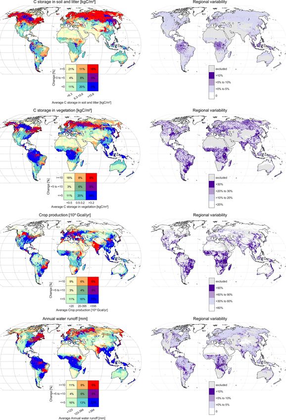
A. D. Bayer et al.: Impact of diverging land-use projections on ecosystems and their service indicators                                     339

Figure 4. The left column shows the categories of the average level of the provision of selected ES indicators in 2000–2004 and the relative
change until 2036–2040 averaged over 16 land-use scenarios. Thresholds for categories for the average ES indicator level follow the 33rd
and 67th percentiles for each ES indicator, whereas the change in indicators is given in 5 % steps for all indicators to allow for comparability.
Note that for soil and litter C, the lowest category is negative. At high levels of ES indicator provision (highest 33 % of values), blue cells
mark regions where little change is expected on average until 2040, and red cells mark regions where high changes are expected until 2040.
The yellow category marks regions where base levels in ES provision are low; therefore, relative changes in these regions can be very high
but are of minor importance. The percentage of global land area in each category is indicated. Cells where the average indicator level in
2000–2004 is zero are colored white and excluded from the statistical analysis. The right column gives the variability of the percent change
in each ES indicator for each cell, which was calculated as the standard deviation of the changes in the ES indicator from 2000–2004 to
2036–2040 that was derived for each of the 16 land-use scenarios individually. Regions where the base level in 2000–2004 was below the
33rd percentile (yellow to green cells in the left column) were excluded from regional variability maps and colored gray in order to focus on
cells with relevant ES indicator provision. Note that the legend scaling is different for vegetation C and crop yield production. Purple regions
indicate a standard deviation in the predicted relative changes in this indicator higher than 10 % of the indicator level in 2000–2004 (30 %
for vegetation C and 90 % for crop yield production). See Fig. S2 for NPP, total C storage and evapotranspiration.

https://doi.org/10.5194/esd-12-327-2021                                                         Earth Syst. Dynam., 12, 327–351, 2021
You can also read