Diversity in Faces - IBM Research
←
→
Page content transcription
If your browser does not render page correctly, please read the page content below
Diversity in Faces
                                                            Michele Merler, Nalini Ratha, Rogerio Feris, John R. Smith
                                                             IBM Research AI @ IBM T. J. Watson Research Center
                                                                       Yorktown Heights, NY 10598, USA
                                                                           Contact: jsmith@us.ibm.com
arXiv:1901.10436v5 [cs.CV] 20 Feb 2019

                                                                                      February 22, 2019

                                                                                            Abstract
                                                   Face recognition is a long-standing challenge in the field of Artificial Intelligence (AI). The
                                               goal is to create systems that detect, recognize, verify and understand characteristics of human
                                               faces. There are significant technical hurdles in making these systems accurate, particularly
                                               in unconstrained settings, due to confounding factors related to pose, resolution, illumination,
                                               occlusion and viewpoint. However, with recent advances in neural networks, face recognition has
                                               achieved unprecedented accuracy, built largely on data-driven deep learning methods. While
                                               this is encouraging, a critical aspect limiting face recognition performance in practice is intrinsic
                                               facial diversity. Every face is different. Every face reflects something unique about us. Aspects
                                               of our heritage – including race, ethnicity, culture, geography – and our individual identity –
                                               age, gender and visible forms of self-expression – are reflected in our faces. Faces are personal.
                                               We expect face recognition to work accurately for each of us. Performance should not vary for
                                               different individuals or different populations. As we rely on data-driven methods to create face
                                               recognition technology, we need to answer a fundamental question: does the training data for
                                               these systems fairly represent the distribution of faces we see in the world? At the heart of this
                                               core question are deeper scientific questions about how to measure facial diversity, what features
                                               capture intrinsic facial variation and how to evaluate coverage and balance for face image data
                                               sets. Towards the goal of answering these questions, Diversity in Faces (DiF ) provides a new
                                               data set of annotations of one million publicly available face images for advancing the study
                                               of facial diversity. The annotations are generated using ten facial coding schemes that provide
                                               human-interpretable quantitative measures of intrinsic facial features. We believe that making
                                               these descriptors available will encourage deeper research on this important topic and accelerate
                                               efforts towards creating more fair and accurate face recognition systems.

                                         1    Introduction
                                         Have you ever been treated unfairly? How did it make you feel? Probably not too good. Most
                                         people generally agree that a fairer world is a better world. Artificial Intelligence (AI) has enormous
                                         potential to make the world a better place. Yet, as we develop and apply AI towards addressing
                                         a broad set of important challenges, we need to make sure the AI systems themselves are fair and
                                         accurate. Recent advances in AI technology have produced remarkable capabilities for accomplish-
                                         ing sophisticated tasks, like translating speech across languages to augment communications and
                                         bridge cultures, improving complex interactions between people and machines, and automatically
                                         recognizing contents of video to assist in safety applications. Much of the recent power of AI comes
                                         from the use of data-driven deep learning to train increasingly accurate models by using growing
                                         amounts of data. However, the strength of these techniques can also be their inherent weakness.

                                                                                                1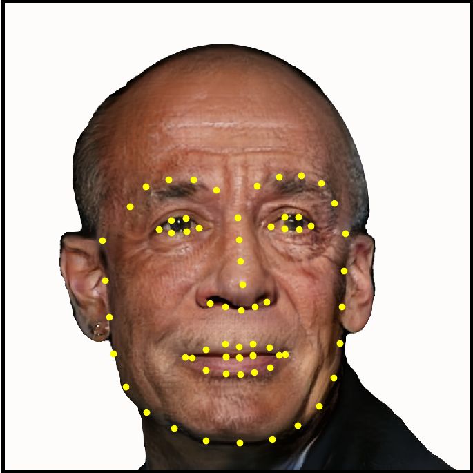
These AI systems learn what they are taught. If they are not taught with robust and diverse data
sets, accuracy and fairness are at risk. For that reason, AI developers and the research community
need to be thoughtful about what data they use for training. This is essential for developing AI
systems which can help to make the world more fair.
    The challenge in training AI systems is manifested in a very apparent and profound way with
face recognition technology. Today, there can be difficulties in making face recognition systems that
meet fairness expectations. The heart of the problem lies not with the AI technology itself, per
se, but with how the systems are trained. For face recognition to perform as desired - to be both
accurate and fair - training data must provide sufficient balance and coverage. The training data
sets should be large enough and diverse enough to learn the many ways in which faces inherently
differ. The images must reflect the diversity of features in faces we see in the world. This raises
the important question of how we measure and ensure diversity for faces. On one hand, we are
familiar with how faces may differ according to age, gender and skin color. But, as prior studies
have shown, these dimensions are inadequate for characterizing the full range of diversity of faces.
Dimensions like face symmetry, facial contrast, and the sizes, distances and ratios of the various
attributes of the face (eyes, nose, forehead, etc.), among many others, are important.
    Diversity in Faces (DiF ) is a new large and diverse data set designed to advance the study of
fairness and accuracy in face recognition technology. DiF provides a data set of annotations of one
million face images. The DiF annotations are made on faces sampled from the publicly available
YFCC-100M data set of 100 million images [1]. The DiF data set provides a comprehensive set of
annotations of intrinsic facial features that includes craniofacial distances, areas and ratios, facial
symmetry and contrast, skin color, age and gender predictions, subjective annotations, and pose and
resolution. The facial coding schemes, summarized in Table 1, are among the strongest identified
in the scientific literature and build a solid foundation to our collective knowledge. We believe that
making these descriptors available will help accelerate the study of diversity and coverage of data
towards creating more fair and accurate face recognition systems.
    In this paper, we describe the development and analysis of the DiF data set. The paper is
organized as follows: in Section 2, we review the state of face recognition technology and examine
how different face image data sets are used today. We discuss some of the shortcomings from
over-reliance on narrow data sets. In Section 3, we describe the process for creating the DiF data
set. In Section 4, we describe the implementation of the ten facial coding schemes. In Section 5,
we provide a statistical analysis of the coding schemes extracted for the face images. In Section 6,
we summarize and discuss future directions.

2        Related Work
Face recognition is a long-standing topic in computer vision, and AI broadly. Computer-based
face recognition was addressed as far back as the 1970s with Takeo Kanade‘s seminal thesis on
recognizing faces using a set of manually defined points corresponding to nose, mouth, eyes and
other features. Modest by today’s standards, his work processed 800 photographs and conducted
experiments involving identification of 20 people [11]. Two decades later, a significant development
came from Matthew Turk and Alex Pentland, who developed an appearance-based technique called
eigenfaces that models faces holistically from image data [12]. This kind of data-driven methodology
was subsequently helped by numerous efforts of curating large and growing face image data sets.
The community has built open evaluations around these data sets, such as MegaFace [13], MS-
Celeb [14] and the NIST Face Recognition Vendor Test (FRVT)1 .
    1
        https://www.nist.gov/programs-projects/face-recognition-vendor-test-frvt

                                                           2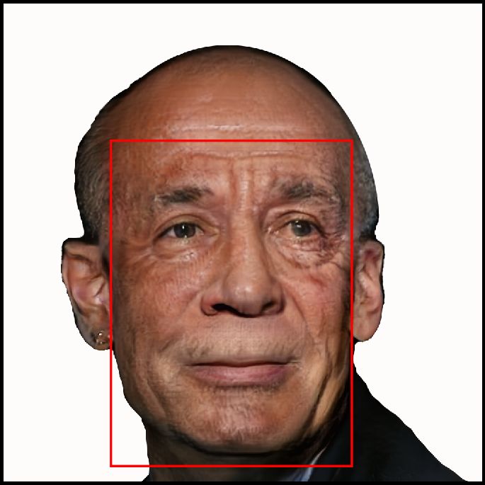
#     Facial Coding Scheme         Reference
                                    L. G. Farkas, Anthropometry of the Head and Face, Raven
 1     Craniofacial Distances
                                    Press, 1994 [2].
                                    L. G. Farkas, et. al, “International anthropometric study of
 2     Craniofacial Areas           facial morphology in various ethnic groups/races,” J Cranio-
                                    fac Surg. 2005 Jul;16(4), pp. 615-46 [3].
                                    N. Ramanathan, R. Chellappa, “Modeling Age Progression in
 3     Craniofacial Ratios          Young Faces,” Intl. Conf. on Computer Vision and Pattern
                                    Recognition (CVPR), 2006, pp. 387-394 [4].
                                    A. C. Little, B. C. Jones, L. M. DeBruine, “Facial attractive-
 4     Facial Symmetry              ness: evolutionary based research,” Philos Trans R Soc Lond
                                    B Biol Sci. 2011 Jun 12;366(1571), pp. 1638-59 [5].
                                    A. Porcheron, E. Mauger, R. Russell, “Aspects of Facial Con-
 5     Facial Contrast              trast Decrease with Age and Are Cues for Age Perception,”
                                    PLoS One 8(3), Mar. 6, 2013 [6].
                                    A. Chardon I. Cretois and C. Hourseau, “Skin colour typol-
 6     Skin Color                   ogy and suntanning pathways,” Intl. Journal of Cosmetic
                                    Science, Aug. 1991, 13(4), pp. 191-208 [7].
                                    R. Rothe, R. Timofte, L. Van Gool, “Deep Expectation of
 7     Age                          Real and Apparent Age from a Single Image Without Facial
                                    Landmarks,” L. Int J Comput Vis (2018) 126: 144 [8].
 8     Gender                       Same as above
                                    Z. Liu, P. Luo, X. Wang, X. Tang, “Deep Learning Face
 9     Subjective Annotation        Attributes in the Wild,” IEEE Intl. Conf. on Computer
                                    Vision (ICCV), 2015 [9]
                                    X. Zhu, D. Ramanan, “Face Detection, Pose Estimation, and
 10    Pose and Resolution          Landmark Localization in the Wild,” Intl. Conf. on Com-
                                    puter Vision and Pattern Recognition (CVPR), 2012 [10].

Table 1: Summary of the ten facial coding schemes used in the DiF data set and their references.

    One prominent example of an early face data set and open evaluation is Labeled Faces in the
Wild (LFW), which is comprised of 13, 233 face photos from the Web of 5, 749 individuals, mostly
celebrities and public figures, captured in unconstrained conditions of lighting, pose and expres-
sion [15]. LFW gained significant focus from the research community upon its release. Eventually,
with the advent of deep learning techniques [16, 17], face recognition performance on LFW reached
near-perfect results with 99.8% accuracy [18,19]. Megaface defined a follow-on larger data set com-
prised of faces from 690, 572 unique individuals which was made more difficult with the addition of
1 million face image distractors [13]. Although early results produced low accuracy in the range of
50% − 60%, ultimately, performance reached near-perfect levels of 99.9% [20, 21]. Other data sets
and evaluations such as CelebA have brought focus to a wider set of problems in face recognition
such as face attribute recognition. CelebA provides a data set of 202, 599 face images with annota-
tions of 40 attributes such as ‘eyeglasses,’ ‘smiling,’ and ‘mustache’ [9]. State-of-art systems have
achieved greater than 90% mean accuracy across the CelebA attribute set and as high as 99% for
some attributes. Many other face data sets and evaluations have produced similar improvements
using deep learning methods [8,9,14,22–34]. The healthy progress on face recognition, as measured
on these data sets and evaluations, has raised expectations in the technology.

                                                 3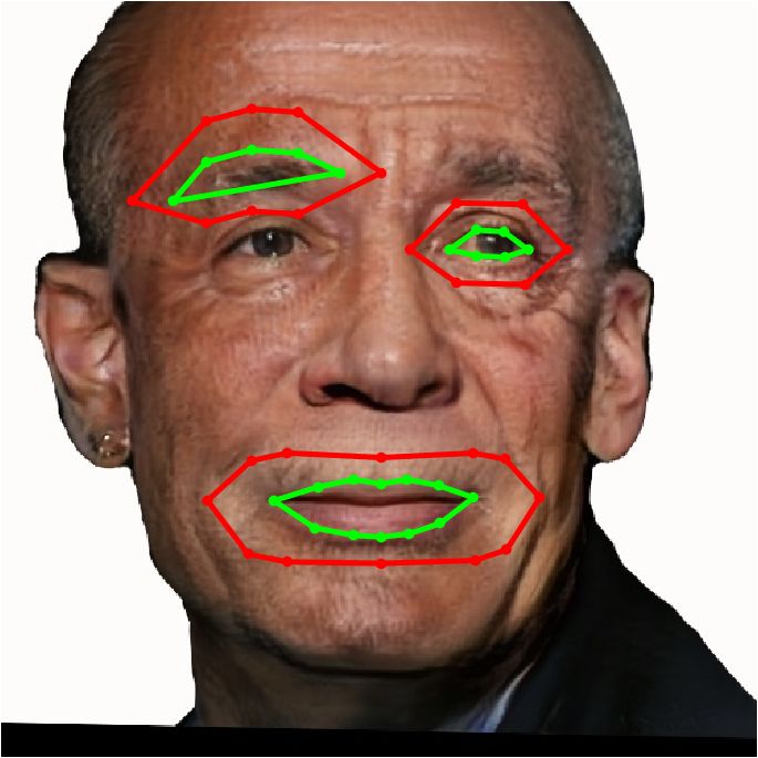
Age Group
           Data set             0-3    4-12    13-19 20-30 31-45 46-60      >60
           LFW [15]            1.0%   10.6%         25.4%      29.6%       33.4%
           IJB-C [28]          0.0%    0.0%     0.5% 16.2% 35.5% 35.1% 12.7%
           Pubfig [35]         1.0%   10.8%         55.5%      21.0%       11.7%
           CelebA [9]                           77.8%                  22.1%
           UTKface [32]        8.8%    6.5%     5.0% 33.6% 22.6% 13.4% 10.1%
           AgeDB [33]          0.1%   0.52%     2.7% 17.5% 31.8% 24.5% 22.9%
           IMDB-Face [24]      0.9%    3.5%    33.2% 36.5% 18.8%    5.4%    1.7%
          Table 2: Distribution of age groups for seven prominent face image data sets.

    However, high accuracy on these data sets does not readily translate into equivalent accuracy
in deployments [36, 37]. The reason is that different or broader distributions of faces, as well as
varied environmental conditions, are found in real applications. Face recognition systems that are
trained within only a narrow context of a specific data set will inevitably acquire bias that skews
learning towards the specific characteristics of the data set. This narrow context appears as under-
representation or over-representation of certain types of faces in many of the publicly available data
sets. Table 2 shows some of the big differences in distribution of age groups for seven prominent
face image data sets. Generally, there is a skew away from younger and older ages. Some of the
differences are quite dramatic. For example, 36.5% of faces in IMDB-Face are for individuals 20-30
years of age, whereas IJB-C has 16.2% of faces in this age group.

                                            Gender          Skin Color/Type
                     Data set           Female Male         Darker Lighter
                     LFW [15]             22.5% 77.4%        18.8%     81.2%
                     IJB-C [28]           37.4% 62.7%        18.0%     82.0%
                     Pubfig [35]          50.8% 49.2%        18.0%     82.0%
                     CelebA [9]           58.1% 42.0%        14.2%     85.8%
                     UTKface [32]         47.8% 52.2%        35.6%     64.4%
                     AgeDB [33]           40.6% 59.5%         5.4%     94.6%
                     PPB [36]             44.6% 55.4%        46.4%     53.6%
                     IMDB-Face [24]       45.0% 55.0%        12.0%     88.0%
  Table 3: Distribution of gender and skin color/type for seven prominent face image data sets.

    Similarly, Table 3 shows the distribution of gender and skin color/type for eight face image data
sets. LFW is highly skewed towards male faces with 77.4% corresponding to male. Six of the eight
data sets have more male faces. A similar skew is seen with skin color/type when grouped coarsely
into darker and lighter groups. Note that different methods were used for characterizing skin
color/type in Table 3, and the meaning of darker and lighter is not the same across these eight data
sets. For all but two data sets the distribution shows > 80% faces that are lighter. AgeDb is the
most heavily skewed, with 94.6% faces that are lighter. The Pilot Parliaments Benchmark (PPB)
data set was designed to be balanced for gender and skin type, where a board certified dermatologist
provided the ground-truth labels using the Fitzpatrick six-point system [36, 38]. However, the age
distribution in PPB is skewed, having been built from official photos of members of parliaments, all
adults, from six countries. Face recognition systems developed from skewed training data are bound

                                                  4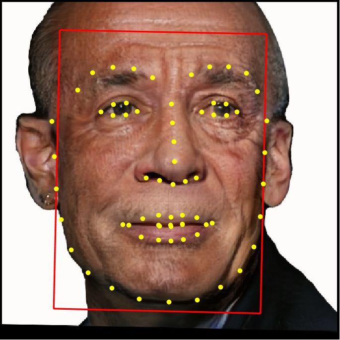
to produce biased models. This mismatch has been evidenced in the significant drop in performance
for different groupings of faces [39–41]. A published study showed that gender estimation from face
images is biased against dark-skinned females over white-skinned males [36, 37]. Such biases may
have serious impacts in practice. Yet much of the prior research on face recognition does not take
these issues under consideration, having focused strongly on driving up accuracy on narrow data
sets. Note also that the gender categorization in Table 3, as in much of the prior work, uses a binary
system for gender classification that corresponds to biological sex – male and female. However,
different interpretations of gender in practice can include biological gender, psychological gender
and social gender roles. As with race and ethnicity, over-simplification of gender by imposing
an incomplete system of categorization can result in face recognition technologies that do not
work fairly for all of us. Some recent efforts, such as InclusiveFaceNet [42], show that imperfect
categorization of race and gender can help with face attribute recognition. However, we expect that
more nuanced treatment of race, ethnicity and gender is important towards improving diversity in
face data sets.

2.1   Bias and Fairness
The study of bias and fairness has recently gained broad interest in computer vision and machine
learning [43–45]. Torralba and Efros [46] presented an evaluation of metrics related to bias and
framed bias in visual classification as a domain transfer problem. Tommasi et al. [47] and Hoffman
et al. [48] conducted a similar evaluation with deep features, showing that data set bias can be
reduced but not eliminated. Khosla et al. [49] proposed a method that learns bias vectors asso-
ciated with individual data sets, as well as weights common across data sets, which are learned
by undoing unwanted bias from each data set. Hardt et al. [50] proposed a framework for fairness
called equalized odds, also referred to as disparate mistreatment [51], where the goal is to predict a
true outcome based on labeled training data, while ensuring it is ‘non-discriminatory’ with respect
to a chosen protected attribute. More recently, Burns et al. [45] addressed bias in image caption-
ing, proposing a model that ensures equal gender probability when gender evidence is occluded in
a scene, and otherwise predicts gender from relevant information when present. The problem of
gender-neutral smile classification was addressed in [42]. Bias in face detection for skin tone, pose
and expression was studied in [52]. Buolamwini et al. [36] proposed an approach to evaluate un-
wanted bias in face recognition and data sets with respect to phenotypic subgroups and introduced
the PPB data set balanced by gender and skin type.

2.2   Face Data Sets
As described above, the last decade has seen an ever-growing collection of face recognition data sets.
Table 4 summarizes many of the prominent face image data sets used for evaluating face recognition
technology. Returning to Labeled Faces in the Wild (LFW) [15], it presented considerable technical
challenges upon its release in 2007, whereas nearly perfect results are being attained today. Several
data sets such as IJBC [53], UMD [26] and VGGFace [22, 23] provide a larger set of face images
with a wider range of pose and lighting variations. Other large-scale face recognition data sets
include MegaFace [13], MS-Celeb [14] and CASIA [25]. Many other data sets have been proposed
for different facial analysis tasks, such as age and gender classification [24, 27, 31, 54–56], facial
expression analysis [55], memorability [57], attributes [35] and aging [58]. Unlike the prior data
sets, which focus on robustness under variations of pose, lighting, occlusion, and scale, the DiF
data set is aimed understanding diversity with respect to intrinsic facial features.

                                                  5
Subj.
Iden- Cranio Cranio Cranio Facial Facial Skin Gen-
Size Age Anno-
Data set -facial -facial -facial Sym- Con- Color/ der Pose
#Images tity tation
Dist. Areas Ratios metry trast Type
MS-Celeb-1M [14] 8.2M y . . . . . . . . . .
Megaface [13] 4.7M y . . . . . . . y y .
VGG2 [22] 3.3M y . . . . . . . y . .
VGG [23] 2.6M y . . . . . . . . . .
IMDB-Face [24] 1.7M y . . . . . . . . . .
annotations (age, gender), and pose.
IMDB-Wiki [8] 523,051 y . . . . . . y y . .
Casia-Webface [25] 494,414 y . . . . . . . y y .
UMDFaces [26] 367,920 y . . . . . . y y . .
CelebA [9] 202,599 . . . . . . . . y y y
CACD [27] 163,446 y . . . . . . y y y .
6
IJB-C [28] 141,332 y . . . . . y y y y y
FaceScrub [29] 105,830 . . . . . . . y y y .
IJB-B [30] 68,195 y . . . . . y y y y y
Pubfig [35] 58,797 y . . . . . . . y y y
Morph [59] 55,134 y . . . . . y y y y .
Adience [31] 26,580 . . . . . . . y y y .
UTKface [32] 24,108 . . . . . . . y y y .
AgeDB [33] 16,488 . . . . . . . y y y .
LFW(A) [15] 13,233 y . . . . . . y y y .
LFW+ [34] 15,699 y . . . . . . . y y .
IJB-A [60] 5,712 y . . . . . . y y y y
PPB [36] 1,270 . . . . . . y . y y .
FGNet [58] 1,002 . . . . . . y y y y .
Diversity in Faces 0.97M . y y y y y y y y y y
and ratios, facial symmetry and contrast, skin color/type, age and gender predictions, subjective
prehensive set of annotations of intrinsic facial features, which include craniofacial distances, areas
Table 4: Summary of prominent face image data sets. The DiF data set provides the most com-3 DiF Data Set Construction
Given the above issues, we were motivated to create the DiF data set to obtain a scientific and
computationally practical basis for ensuring fairness and accuracy in face recognition. At one
extreme the challenge of diversity could be solved by building a data set comprised from the face
of every person in the world. However, this would not be practical or even possible, let alone the
significant privacy concerns. For one, our facial appearances are constantly changing due to ageing,
among other factors. At best this would give a solution for a point in time. Rather, a solution
needs to come from obtaining or generating a representative sample of faces with sufficient coverage
and balance. That, however, is also not a simple task. There are many challenging questions: what
does coverage mean computationally? How should balance be measured? Are age, gender and skin
color sufficient? What about other highly personal attributes that are part of our identity, such as
race, ethnicity, culture, geography, or visible forms of self-expression that are reflected in our faces
in a myriad of ways? We realized very quickly that until these questions were answered we could
not construct a complete and balanced data set of face images.
We formulated a new approach that would help answer these questions. We designed the
DiF data set to provide a scientific foundation for research into facial diversity. We reviewed
the scientific literature on face analysis and studied prior work in fields as diverse as psychology,
sociology, dermatology, cosmetology and facial surgery. We concluded that no single facial feature
or combination of commonly used classifications – such as age, gender and skin color – would
suffice. Therefore, we formulated a novel multi-modal approach that incorporates a diversity of face
analysis methods. Based on study of the large body of prior work, we chose to implement a solid
starter-set of ten facial coding schemes. The criteria for selecting these coding schemes included
several important considerations: (1) strong scientific basis as evidenced by highly cited prior work,
(2) extracting the coding scheme was computationally feasible, (3) the coding scheme produced
continuous valued dimensions that could feed subsequent analysis, as opposed to generating only
categorical values or labels, and (4) the coding scheme would allow for human interpretation to
help with our understanding.
We chose YFCC-100M [1] to be the source for the sample of images. There were a number
of important reasons for this. Ideally, we would be able to automatically obtain any large sample
of images from any source meeting any characteristics of diversity we desire. However, practical
considerations prevent this, including the fact that various copyright laws and privacy regulations
must be respected. YFCC-100M is one of the largest image collections, consisting of more than 100
millions photos. It was populated by users of the Flickr photo service. There is a large diversity
in these photos overall, where people and faces appear in an enormous number of ways. Also,
importantly, a large portion of the photos have Creative Commons license. The downside of using
YFCC-100M is that there is skew in the Flickr user community that contributed the photos. We
cannot rely on the set of users or their photos to be inherently diverse. A consequence of this is
that the set of images used in the DiF is not completely balanced on its own. However, it still
provides the desired basis for studying methods for characterizing facial diversity.
3.1 Data Selection
While the YFCC-100M photo data set is large, not all images could be considered. Naturally, we
excluded photos that did not contain a face. We also excluded black and white and grayscale photos
and those with significant blur. Although face recognition needs to be robust for non-color photos,
we deferred incorporating these images in the initial DiF data set in order to focus on intrinsic
facial variation rather than image variation due to color processing.
7(a) face detection (size) (b) face keypoints (pose and iod) (c) face rectification
Figure 1: Each candidate photo from YFCC-100M was processed by first detecting the depicted
faces with a Convolutional Neural Network (CNN) using the Faster-RCNN based object detec-
tor [61]. Then each detected face as in (a) was processed using DLIB [62] to extract pose and
landmark points as shown in (b) and subsequently assessed based on the width and height of the
face region. Faces with region size less than 50x50 or inter-ocular distance of less than 30 pixels
were discarded. Faces with non-frontal pose, or anything beyond being slightly tilted to the left or
the right, were also discarded. Finally, an affine transformation was performed using center points
of both eyes, and the face was rectified as shown in (c).
3.2 Pre-processing Pipeline
The YFCC-100M data set gives a set of URLs that point to the Flickr web page for each of the
photos. The first step we took was to check whether the URL was still active. If so, we then checked
the license. We proceeded with the download only if the license type was Creative Commons. Once
we retrieved the photo, we processed it using face detection to find all depicted faces. For the
face detection step, we used a Convolutional Neural Network (CNN) object detector trained for
faces based on Faster-RCNN [61]. For each detected face, we then extracted both pose and 68
face key-points using the open source DLIB toolkit [62]. If there was any failure in the image
processing steps, we excluded the face from further consideration. We also removed faces of size
less than 50 × 50 pixels or with inter-ocular distance of less than 30 pixels. We removed faces with
substantial non-frontal pose. The overall process is shown in Figure 1.
Finally, we generated two instances of each face. One is a rectified instance whereby the center
points of each eye are fixed to a specific location in the overall image. The second crops an expanded
region surrounding each face to give 50% additional spatial context. This overall process filtered
the 100 million YFCC-100M photos down to approximately one million mostly frontal faces with
adequate size. The surviving face images were the ones used for the DiF data set. Note that the
overall process of sampling YFCC-100M used only factors described above including color, size,
quality and pose. We did not bias the sampling towards intrinsic facial characteristics or by using
metadata associated with each photo, such as a geo-tag, date, labels or Flickr user name. In this
sense, the DiF data distribution is expected to closely follow the overall distribution of the YFCC-
100M photos. In future efforts to grow the DiF data set, we may relax some of the constraints
based on size, pose and quality, or we may bias the sampling based on other properties. However,
one million publicly available face images provides a good start. Given this compiled set of faces,
we next process each one by extracting the ten facial coding schemes.
84 Facial Coding Scheme Implementation
In this Section, we describe the implementation of the ten facial coding schemes and the process
of extracting them from the DiF face images. The advantage of using ten coding schemes is that
it gives a diversity of methods and allows us to compare statistical measures for facial diversity.
As described above, the ten schemes have been selected based on their strong scientific basis, com-
putational feasibility, numerical representation and interpretability. Overall the chosen ten coding
schemes capture multiple modalities of facial features, which includes craniofacial distances, areas
and ratios, facial symmetry and contrast, skin color, age and gender predictions, subjective anno-
tations, and pose and resolution. Three of the DiF facial coding schemes are based on craniofacial
features. As prior work has pointed out, skin color alone is not a strong predictor of race, and
other features such as facial proportions are important [6, 63–65]. Face morphology is also relevant
for attributes such as age and gender [4]. We incorporated multiple facial coding schemes aimed
at capturing facial morphology using craniofacial features [2–4]. The basis of craniofacial science
is the measurement of the face in terms of distances, sizes and ratios between specific points such
as the tip of the nose, corner of the eyes, lips, chin, and so on. Many of these measures can be
reliably estimated from photos of frontal faces using 47 landmark points of the head and face [2].
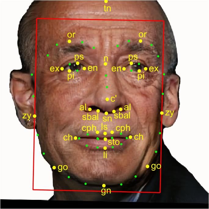
To provide the basis for the three craniofacial feature coding schemes used in DiF , we built on the
subset of 19 facial landmarks listed in Table 5. For brevity we adopt the abbreviations from [2]
when referring to these facial landmark points instead of using the full anatomical terms.
Anatomical term Abbreviation Anatomical term Abbreviation
tragion tn subalare sbal
orbitale or subnasale sn
palpebrale superius ps crista philtre cph
palpebrale inferius pi labiale superius ls
endocanthion en stornion sto
exocanthion ex labiale inferius li
nasion n chelion ch
pronasale c0 gonion go
zygion zy gnathion gn
alare al
Table 5: Anatomical terms and corresponding abbreviations (as in [2]) for the set of facial landmarks
employed to compute the craniofacial measurements for facial coding schemes 1–3.
In order to extract the 19 facial landmark points, we leveraged standard DLIB facial key-point
extraction tools that provide a set 68 key-points for each face. As shown in Figure 2, we mapped the
68 DLIB key-points to the 19 facial landmarks [2]. These 19 landmarks were used for extracting
the craniofacial features. Note that for illustrative purposes, the example face used in Figure 2
was adopted from [66] and was generated synthetically using a progressive Generative Adversarial
Network (GAN) model. The face does not correspond to a known individual person. However,
the image is subject to license terms as per [66]. In order to incorporate a diversity of approaches,
we implemented three facial coding schemes for craniofacial features. The first, coding scheme 1,
provides a set of craniofacial distance measures from [2]. The second, coding scheme 2, provides an
expanded set of craniofacial areas from [3]. The third, coding scheme 3, provides a set of craniofacial
ratios from [4].
9Figure 2: We used the 68 key-points extracted using DLIB from each face (small dots) to localize
19 facial landmarks (large dots, labeled), out of the 47 introduced in [2]. Those 19 landmarks were
employed as the basis for extraction of the craniofacial measures for coding schemes 1–3.
4.1 Coding Scheme 1: Craniofacial Distances
The first coding scheme for craniofacial distances has been adopted from [2]. It comprises eight
measures which characterize all the vertical distances between elements in a face: the top of the
forehead, the eyes, the nose, the mouth and the chin. In referring to the implementation of the
coding scheme, we use the abbreviations from Table 5. We note that two required points, tn and
sto, were not part of the set of 68 DLIB key-points. As such, we had to derive them in the following
manner: tn was computed as the topmost point vertically above n in the rectified facial image,
and sto was computed from the vertical average of ls and li. The eight dimensions of craniofacial
distances are summarized in Table 6.
4.2 Coding Scheme 2: Craniofacial Areas
The second coding scheme is adopted from a later development from Farkas et al. [3]. It comprises
measures corresponding to different areas of the cranium. Similar to the craniofacial distances, the
extraction of craniofacial areas relied on the mapped DLIB key-points to the corresponding facial
landmarks. Table 7 summarizes the twelve dimensions of the craniofacial area features.
10Craniofacial distance Measure
intercanthal face height n − sto
eye fissure height (left and right) ps − pi
orbit and brow height (left and right) or − pi
columella length sn − c0
upper lip height sn − sto
lower vermilion height sto − li
philtrum width cph − cph
lateral upper lip heights (left and right) sbal − ls0
Table 6: Coding scheme 1 is made up eight craniofacial measures corresponding to different vertical
distances in the face [2].
Craniofacial area Measure
Head height tn − n
Face height tn − gn
Face height n − gn
Face height sn − gn
Face width zy − zy
Face width go − go
Orbits intercanthal width en − en
Orbits fissure length (left and right) en − ex
Orbits biocular width ex − ex
Nose height n − sn
Nose width al − al
Labio-oral region ch − ch
Table 7: Coding scheme 2 is made up of twelve craniofacial measures that correspond to different
areas of the face [3].
4.3 Coding Scheme 3: Craniofacial Ratios
The third coding scheme comprises measures corresponding to different ratios of the face. These
features were used to estimate age progression from faces in the age groups of 0 to 18 in [4]. Similar
to the above features, the craniofacial ratios used the mapped DLIB key-points as facial landmarks.
Table 8 summarizes the eight dimensions of the craniofacial ratio features.
4.4 Coding Scheme 4: Facial Symmetry
Facial symmetry has been found in psychology and anthropology studies to be correlated with
subjective and objective traits including expression variation [67] and attractiveness [5]. We adopted
facial symmetry for coding scheme 4, given its intrinsic nature. To represent the symmetry of each
face we computed two measures, following the work of Liu et al. [67]. We processed each face as
shown in Figure 3. We used three of the DLIB key-points detected in the face image to spatially
normalize and rectify it to the following locations: the inner canthus of each eye (C1 and C2) to
reference locations C1 = (40, 48), C2 = (88, 48) and the philtrum C3 was mapped to C3 = (64, 84).
Next, the face mid-line (point b in Figure 3(a)) was computed as the line passing through the
mid-point of the line segment connecting C1 − C2 (point a in Figure 3(a)) and the philtrum C3.
11Craniofacial ratio Measure
Facial index (n − gn)/(zy − zy)
Mandibular index (sto − gn)/(go − go)
Intercanthal index (en − en)/(ex − ex)
Orbital width index (left and right) (ex − en)/(en − en)
Eye fissure index (left and right) (ps − pi)/(ex − en)
Nasal index (al − al)/(n − sn)
Vermilion height index (ls − sto)/(sto − li)
Mouth-face width index (ch − ch)/(zy − zy)
Table 8: Coding scheme 3 is made up of eight craniofacial measures that correspond to different
ratios of the face [3].
(a) (b) (c)
Figure 3: Process for extracting facial symmetry measures for coding scheme 4, starting with (a)
rectified face showing face mid-line and reference points for inner canthus (C1 and C2) and philtrum
(C3) and line segmented connecting them (point a for C1-C2 and point b connecting C3 to the
midpoint of point a). Additionally, a Sobel filter is used to extract (b) edge magnitude and (c)
orientation to derive the measure for edge orientation similarity.
We point out that although a face image is spatially transformed during rectification, facial
symmetry with respect to the face mid-line is preserved according to the topological properties of
the affine transformation [68]. Each image is then cropped to 128x128 pixels to create a squared
image with the face mid-line centered vertically. Next we convert the spatially transformed image
to grayscale to measure intensity. Each point (x, y) on this normalized face intensity image I
on the left of the face mid-line has a unique corresponding horizontally mirrored point on the
other side of the face image I 0 (x, y) (right of the mid-line). We also extract edges in this image
I to produce Ie using a Sobel filter. Finally, we compute two facial symmetry measures based on
density difference DD(x, y) and edge orientation similarity EOS(x, y) as follows: for each pixel
(x, y) in the left 128x64 part (I and Ie ) and the corresponding 128x64 right part (I 0 and Ie0 ) are
computed as summarized in Table 9, where φ(Ie (x, y), Ie0 (x, y)) is the angle between the two edge
orientations of images Ie and Ie0 at pixel (x, y). We compute the average value of DD(x, y) and
EOS(x, y) to be the two measures for facial symmetry.
It is interesting to notice that the two symmetry measurements capture facial symmetry from
different perspectives: density difference is affected by the left-right relative intensity variations of
a face, while edge orientation similarity is affected by the zero-crossing of the intensity field. Higher
values of density difference correspond to more asymmetrical faces, while the higher the values of
edge orientation similarity refer to more symmetrical faces.
12Facial symmetry Measure
Density difference DD(x, y) = I(x, y) − I 0 (x, y)
Edge orientation similarity EOS(x, y) = cos(φ(Ie (x, y), Ie0 (x, y)))
Table 9: Coding scheme 4 is made up of two measures of facial symmetry [3].
4.5 Coding Scheme 5: Facial Regions Contrast
Prior studies have shown that facial contrast is a cross-cultural cue for perceiving facial attributes
such as age. An analysis of full face color photographs of Chinese, Latin American and black South
African women aged 20–80 in [6] found similar changes in facial contrast with ageing across races
and were comparable to changes with Caucasian faces. This study found that high-contrast faces
were judged to be younger than low-contrast faces. The study also found that artificially increasing
the aspects of facial contrast that decrease with age across diverse races makes faces look younger,
independent of the ethnic origin of the face or cultural origin of the observers [6]. On one hand,
the age that you are is one dimension that needs to be addressed in terms of fairness and accuracy
of face recognition. However, the age that you look, considering possible artificial changes, should
not change requirements for fairness and accuracy.
Figure 4: Process for extracting facial regions contrast measures for coding scheme 5. The compu-
tation is based on the average pixel intensity differences between the outer and inner regions for
the lips, eyes and eyebrows as depicted above.
We adopted facial regions contrast as the basis for coding scheme 5. To compute facial contrast,
we measured contrast individually for each image color channel IL , Ia , Ib , corresponding to the CIE-
Lab color space, for three facial regions: lips, eyes, and eyebrows, as shown in Figure 4. First, we
defined the internal regions ringed by facial key points computed from DLIB for each of these facial
parts (shown as the inner rings around lips, eyes, and eyebrows in Figure 4). Then, we expanded this
region by 50% to define an outer region around each of these facial parts (shown as the outer rings
in Figure 4). The contrast is then measured as the difference between the average pixel intensities
in the outer and inner regions. This is repeated for each of the three CIE-Lab color channels.
Given the three facial regions, this gives a total of nine measures, where the contrast values for
the eyes and eyebrows are based on the average of the left and right regions. The computation is
summarized in Table 10, where Ik (x, y) is the pixel intensity at (x, y) for CIE-Lab channel k and
ptouter , ptinner correspond to the outer and inner regions around each facial part pt.
13Facial region contrast Measure
P P
IL (x,y)− IL (x,y)
Lips CIE-L CL,lips = Px,y∈lipsouter IL (x,y)+Px,y∈lipsinner IL (x,y)
Px,y∈lipsouter P x,y∈lipsinner
x,y∈lipsouter Ia (x,y)− x,y∈lipsinner Ia (x,y)
Lips CIE-a Ca,lips = P P
I (x,y)+ x,y∈lips Ia (x,y)
Px,y∈lipsouter a P inner
x,y∈lipsouter Ib (x,y)− x,y∈lipsinner Ib (x,y)
Lips CIE-b Cb,lips = P P
I (x,y)+ x,y∈lips I (x,y)
P x,y∈lipsouter b P inner b
I L (x,y)− IL (x,y)
Eyes CIE-L CL,eyes = Px,y∈eyesouter IL (x,y)+Px,y∈eyesinner IL (x,y)
Px,y∈eyesouter P x,y∈eyesinner
x,y∈eyesouter Ia (x,y)− x,y∈eyesinner Ia (x,y)
Eyes CIE-a Ca,eyes = P P
I (x,y)+ x,y∈eyes Ia (x,y)
Px,y∈eyesouter a P inner
x,y∈eyesouter Ib (x,y)− x,y∈eyesinner Ib (x,y)
Eyes CIE-b Cb,eyes = P P
I (x,y)+ x,y∈eyes I (x,y)
P x,y∈eyesouter b P inner b
x,y∈eyebrowsouter IL (x,y)− x,y∈eyebrowsinner IL (x,y)
Eyebrows CIE-L CL,eyebrows = P P
I (x,y)+ x,y∈eyebrows IL (x,y)
Px,y∈eyebrowsouter L P inner
x,y∈eyebrowsouter Ia (x,y)− x,y∈eyebrowsinner Ia (x,y)
Eyebrows CIE-a Ca,eyebrows = P P
I (x,y)+ x,y∈eyebrows Ia (x,y)
Px,y∈eyebrowsouter a P inner
Ib (x,y)− I b (x,y)
Eyebrows CIE-b Cb,eyebrows = Px,y∈eyebrowsouter Ib (x,y)+Px,y∈eyebrowsinner Ib (x,y)
x,y∈eyebrows outer x,y∈eyebrows inner
Table 10: Coding scheme 5 is made up of three measures of facial region contrast [6].
4.6 Coding Scheme 6: Skin Color
Skin occupies a large fraction of the face. As such, characteristics of the skin influence the appear-
ance and perception of faces. Prior work has studied different methods of characterizing skin based
on skin color [7, 69, 70], skin type [7, 38] and skin reflectance [71]. Early studies used Fitzpatrick
skin type (FST) to classify sun-reactive skin types [38], which was also adopted recently in [36].
However, to-date, there is no universal measure for skin color, even within the dermatology field. In
a study of 556 participants in South Africa, self-identified as either black, Indian/Asian, white, or
mixed, Wilkes et al. found a high correlation between the Melanin Index (MI), which is frequently
used to assign FST, with Individual Typology Angle (ITA) [72]. Since a dermatology expert is
typically needed to assign the FST, the high correlation of MI and ITA indicates that ITA may
be a practical method for measuring skin color given the simplicity of computing ITA. In order to
explore this further, we designed coding scheme 6 to use ITA for representing skin color [7]. ITA
has a strong advantage over Fitzpatrick in that it can be computed directly from an image. As
in [7], we implemented ITA in the CIE-Lab space. For obvious practical reasons, we could not
obtain measurements through a device directly applied on the skin of each individual, but instead
converted the RGB image to CIE-Lab space using standard image processing. The L axis quan-
tifies luminance, whereas a quantifies absence or presence of redness, and b quantifies yellowness.
Figure 5 depicts the image processing steps for extracting the coding scheme 6 for skin color.
It is important to note that that ITA is a point measurement. Hence, every pixel corresponding
to skin can have an ITA measurement. In order to generate a feature measure for the whole face,
we extract ITA for pixels within a masked face region as shown in Figure 5(g). This masked region
is determined in the following steps:
1. Extract the skin mask in the face (pixels corresponding to skin) using a deep neural network,
as described in [73].
2. Extract regions corresponding to the chin, two cheeks and forehead using the extracted 68
DLIB key-points
14(a) (b) (c) (d)
700
600
Histogram moving average count
500
400
300
200
100
0
-90 -80 -70 -60 -50 -40 -30 -20 -10 0 10 20 30 40 50 60 70 80 90
ITA
(e) (f) (g) (h)
Figure 5: Process for extracting skin color for coding scheme 6 based on Individual Typology
Angle-based (ITA). (a) Input face (b) skin map (c) L channel (d) a channel (e) b channel (f) ITA
map (g) masked ITA map (h) ITA histogram.
3. Smooth the ITA values of each region to reduce outliers using an averaging filter
4. Pick the peak value of each region to give its ITA score
5. Average the values to give a single ITA score for each face
Table 11 gives the formula for computing the ITA values for each pixel in the masked face region.
Skin color Measure
arctan( L−50 )×180
Individual Typology Angle (ITA) π
b
Table 11: Coding scheme 6 measures skin color using Individual Typology Angle (ITA) [3].
4.7 Coding Scheme 7: Age Prediction
Age is an attribute we all possess and our faces are predictors of our age, whether it is our actual
age or manipulated age appearance [6]. As discussed in Section 4.5, particular facial features
such as facial contrast are correlated with age. As an alternative to designing specific feature
representations for predicting age, for coding scheme 7, we adopt a Convolutional Neural Network
(CNN) that is trained from face images to predict age. We adopt the DEX model [8, 74] that is
among the highest performing on some of the known face image data sets. The model is based
on a pre-trained VGG16-face neural network for face identity that was subsequently fine-tuned on
the IMDB-wiki data set [8] to predict age (years in the range 0-100). Since the DEX model was
trained within a narrow context, it is not likely to be fair. However, our initial use here is to get
some continuous measure of age in order to study diversity. Ultimately, it will require an iterative
process of understanding diversity to make more balanced data sets and create more fair models.
In order to predict age using DEX, each face was pre-processed as in [74]. First, the bounding box
15was expanded by 40% both horizontally and vertically, then resized to 256x256 pixels. Inferencing
was then performed on the 224x224 square cropped at the center of the image. Since softmax loss
was used during the fine-tuning process, age prediction is output from the softmax layer, which is
computed from E(P ) = 100
P
i=0 i yi , where pi ∈ P are the softmax output probabilities for each of
p
the 101 discrete years yi ∈ Y corresponding to each class i, with Y = {0, ..., 100}.
4.8 Coding Scheme 8: Gender Prediction
Coding scheme 8 follows a similar process for gender prediction as for age prediction [8]. We used
the same pre-processing steps as described in Section 4.7 as well as the same neural network model
and training pipeline. The only difference is that we use the DEX model to predict a continuous
value score for gender between 0 and 1, and not just report a binary output.
4.9 Coding Scheme 9: Subjective Annotation
Coding scheme 9 aims at capturing age and gender but through subjective means rather than using
a neural network-based predictive model. For each of the DiF face images, we employed the Figure
Eight crowd-sourcing platform [75] to obtain subjective human-labeled annotations of gender and
age. The gender annotations used two class labels (male and female) and the age group labeling
used seven classes ([0-3],[4-12],[13-19],[20-30],[31-45],[46-60],[61-]), as well as a continuous age value
to be consistent with the automatic prediction labels. For each face, input was taken from three
independent annotators. A weighted voting scheme was used to aggregate the labels, where the
vote of each annotator was weighted according to their performance on a set of “gold standard”
faces for which the ground truth was known.
4.10 Coding Scheme 10: Pose and Resolution
The final coding scheme 10 provides information about pose and resolution. Although pose can
only loosely be considered an intrinsic facial attribute, how we present our faces to cameras should
not affect performance. We include resolution as it gives useful information to correlate with the
other coding scheme features to provide further insight. In order to extract pose, we use the DLIB
toolkit to compute a pose score of 0-4. Here, the values correspond as follows: 0-frontal, 1-rotated
left, 2-rotated right, 3-frontal but tilted left, 4-frontal but tilted right. Along with pose, resolution
is determined from the size of the bounding box of each face and inter-ocular distance (IOD), which
is the distance between the center points of each eye.
5 Statistical Analysis
In this Section, we report on the statistical analysis of the ten facial coding schemes in the DiF
data set. Intuitively, in order to provide sufficient coverage and balance, a data set needs to include
data with diverse population characteristics. This type of analysis comes up in multiple disciplines,
including bio-diversity [76, 77], where an important objective is to quantify species diversity of
ecological communities. It has been reported that species diversity has two separate components:
(1) species richness, or the number of species present, and (2) their relative abundances, called
evenness. We use these same measures to quantify the diversity of face images using the ten facial
coding schemes. We compute diversity using Shannon H and E scores and Simpson D and E
scores [76]. Additionally, we measure mean and variance for each of the feature dimensions of
the ten facial coding schemes The computation of diversity is as follows: given individual pi in a
16probability distribution for each feature measure, and the S being the number of classes for the
attribute, we compute:
Diversity Evenness
PS H
Shannon H = − i=1 pi ∗ ln(pi ) Shannon E = ln(S)
Simpson D = PS 1 Simpson E = D
S
i=1 (pi ∗pi )
Shannon H and Simpson D are diversity measures and Shannon E and Simpson E are evenness
measures. To see how they work, consider a 20 class problem (S = 20) with uniform distribution
(pi = 0.05). These measures take the following values: Shannon H = 2.999, Shannon E = 1.0,
Simpson D = 2.563, and Simpson E = 1.0. Evenness is constant at 1.0 as expected. Shannon D
represents the diversity of 20 classes (e2.999 ≈ 20). For complex distributions, it may not be easy
to understand the meaning of specific values of these scores. Generally, a higher diversity value is
better than a lower value, whereas an evenness value closer to 1.0 is better. Figure 6 illustrates
these measures on two example distributions. Figure 6 (a) and (b) show how diversity and evenness
values vary for a uniform distribution, respectively, as the number of classes increase from 2 to 20.
Figure 6 (c) and (d) show the same information for a random distribution.
Table 12 summarizes the diversity scores computed for the ten facial coding schemes in the DiF
data set. As described in Section 4, many of the coding schemes have multiple dimensions. Hence
the table has more than ten rows. The craniofacial measurements across the three coding scheme
types total 28 features corresponding to craniofacial distances, craniofacial areas and craniofacial
ratios. The diversity scores of the different dimensions of the remaining seven coding schemes can
similarly be seen in Table 12.
5.1 Coding Scheme 1: Craniofacial Distances
Figure 7 summarizes the feature distribution for the 8 craniofacial distances in coding scheme 1.
The highest Simpson D value is 5.887 and the lowest is 5.83. The highest and lowest Shannon H
values are 1.786 and 1.77. Based on the Shannon H values, this feature dimension would typically
map to 6 classes. Evenness is generally balanced with highest Simpson E and Shannon E of 0.98
and 0.994, respectively.
(a) (b) (c) (d)
Figure 6: Illustration of how (a) diversity and (b) evenness varies for a uniform distribution com-
pared to how (c) diversity and (d) evenness varies for a random distribution.
17Coding
Measurement Simp. D Simp. E Shan. H Shan. E Mean Var
Scheme
n − sto 5.875 0.979 1.781 0.994 33.20 3.93
ps − pi 5.887 0.981 1.782 0.995 3.26 0.98
or − sci 5.867 0.978 1.780 0.994 12.65 2.22
Craniofacial sn − cc 5.832 0.972 1.777 0.992 6.50 1.69
Distance sn − sto 5.870 0.978 1.780 0.994 9.95 2.13
sto − li 5.862 0.977 1.780 0.994 5.86 1.98
cph − cph 5.873 0.979 1.781 0.994 6.99 1.35
sbal − lss 5.832 0.972 1.777 0.992 7.07 1.63
tn − n 5.887 0.981 1.782 0.995 33.83 5.25
tn − gn 5.879 0.980 1.781 0.994 89.28 9.45
n − gn 5.878 0.980 1.781 0.994 55.45 7.49
sn − gn 5.877 0.980 1.781 0.994 32.20 5.82
zy − zy 5.869 0.978 1.780 0.994 63.67 4.44
Craniofacial go − go 5.888 0.981 1.782 0.995 43.47 3.90
Area en − en 5.875 0.979 1.781 0.994 17.49 1.06
en − ex 5.880 0.980 1.781 0.994 11.56 0.56
ex − ex 5.882 0.980 1.782 0.994 40.62 1.02
n − sn 5.873 0.979 1.781 0.994 23.24 3.02
al − al 5.876 0.979 1.781 0.994 13.62 1.65
ch − ch 5.858 0.976 1.78 0.993 27.09 4.05
(n − gn)/(zy − zy) 5.878 0.980 1.781 0.994 0.87 0.11
(sto − gn)/(go − go) 5.878 0.980 1.781 0.994 0.51 0.09
(en − en)/(ex − ex) 5.885 0.981 1.782 0.995 0.43 0.02
Craniofacial (ex − en)/(en − en) 5.870 0.978 1.781 0.994 0.66 0.06
Ratio (ps − pi)/(ex − en) 5.878 0.980 1.781 0.994 0.28 0.08
(al − al)/(n − sn) 5.903 0.984 1.783 0.995 0.59 0.08
(ls − sto)/(sto − li) 5.884 0.981 1.782 0.994 0.67 0.34
(ch − ch)/(zy − zy) 5.873 0.979 1.781 0.994 0.42 0.06
Facial Density difference 4.777 0.796 1.620 0.904 0.12 0.06
Symmetry Edge or. similarity 5.005 0.834 1.692 0.944 0.01 0.01
Lips L contrast 5.857 0.976 1.779 0.993 -0.07 0.09
Lips a contrast 5.781 0.963 1.772 0.989 0.02 0.02
Lips b contrast 5.867 0.978 1.780 0.994 -0.01 0.01
Eyes L contrast 5.725 0.954 1.766 0.986 -0.18 0.14
Facial
Eyes a contrast 5.872 0.979 1.781 0.994 -0.02 0.01
Contrast
Eyes b contrast 5.862 0.977 1.780 0.993 -0.02 0.02
Eb L contrast 5.722 0.954 1.766 0.986 -0.11 0.11
Eb a contrast 5.759 0.960 1.769 0.987 -0.01 0.01
Eb b contrast 5.666 0.944 1.760 0.982 -0.01 0.01
Skin Color ITA 5.281 0.754 1.773 0.911 14.02 45.12
Age Age prediction 4.366 0.624 1.601 0.823 26.29 14.64
Gender Gender prediction 3.439 0.573 1.488 0.831 0.27 0.32
Subjective Gender labeling 2.000 1.000 0.693 1.000 0.49 0.50
Annotation Age labeling 4.395 0.628 1.675 0.861 30.45 16.98
Pose Pose 1.224 0.408 0.390 0.355 -0.01 0.31
& IOD 4.993 0.832 1.692 0.944 43.64 22.15
Resolution Face Region Size 2.819 0.470 1.198 0.668 93.37 42.98
Table 12: Summary of facial coding scheme analysis for the DiF data set using Simpson D (diver-
sity), Simpson E (evenness), Shannon H (diversity), Shannon E (evenness), mean and variance.
18Figure 7: Feature distribution of craniofacial distances (coding scheme 1) for the DiF data set.
5.2 Coding Scheme 2: Craniofacial Areas
Figure 8 summarizes the feature distribution for the 12 craniofacial areas in coding scheme 2. The
highest Simpson D value is 5.887 and the smallest is 5.879. The highest Shannon D value is 1.782
and the lowest is 1.78. Compared to coding scheme 1, these values are in the similar range, mapping
to 6 classes. Evenness ranges between 0.98 and 0.976.
5.3 Coding Scheme 3: Craniofacial Ratios
Figure 9 summarizes the feature distribution for the 8 craniofacial ratios in coding scheme 3. Unlike
the previous coding scheme 2, the diversity values for this coding schemes have less variance. The
largest Simpson D value is 5.9 and smallest is 5.87. Similarly, the largest Shannon H value is 1.782
and smallest is 1.781. This would map to approximately to 6 classes. While Simpson E has a range
between 0.979 to 0.984, Shannon E ranges between 0.995 to 0.994. The evenness of coding scheme
3 is similar to coding scheme 2.
5.4 Coding Scheme 4: Facial Symmetry
Figure 10 summarizes the feature distribution for facial symmetry in coding scheme 4. The diversity
value is in a middle range compared to the previous coding schemes. For example, the highest
Simpson D is 5.05 and the largest Shannon H is 1.69. The evenness values are lower as well with
highest Simpson E value being 0.834 and highest Shannon E value being 0.944. The Shannon H
value of 1.69 translates to about 5.4 classes.
5.5 Coding Scheme 5: Facial Regions Contrast
Figure 11 summarizes the feature distribution for facial contrast in coding scheme 5. The highest
Simpson D value is 5.872 and highest Shannon H value is 1.781, which is equivalent to 5.9 classes.
The evenness factor Shannon E is very close to 0.979 indicating that the measures are close to
even.
19Figure 8: Feature distribution of craniofacial areas (coding scheme 2) for the DiF data set.
5.6 Coding Scheme 6: Skin Color
Figure 12 summarizes the feature distribution for skin color in coding scheme 6. The Simpson D
value is 5.28 and Shannon H value is 1.77 which translates to about 5.88 classes, which shows a
good match with the number of bins we used. The evenness is weaker than a uniform distribution.
5.7 Coding Scheme 7: Age Prediction
Figure 13(a) summarizes the feature distribution for age prediction in coding scheme 7, where we
bin the age values into seven groups: [0-3],[4-12],[13-19],[20-30],[31-45],[46-60],[61-]. The Simpson
D and Shannon H values are 4.37 and 1.6. Because of the data distribution not being even, we
can see a lower E value around 0.62. The Shannon H value of 1.61 maps to 5 classes.
5.8 Coding Scheme 8: Gender Prediction
Figure 13 also summarizes the feature distribution for gender prediction in coding scheme 8. Even
though this has two classes, male and female, the confidence score ranges between 0−1. The gender
score distribution is shown in Figure 13 (b). The Simpson D is 3.43 and Shannon H is 1.49. The
Shannon H value translates to 4.4 classes, which is beyond the typical two classes used for gender,
possibly reflecting the presence of sub-classes. The Shannon evenness score of 0.57 reflect some
unevenness as well.
5.9 Coding Scheme 9: Subjective Annotation
Figure 14 summarizes the feature distribution for the subjective annotations of age and gender for
coding scheme 9. The Simpson D for gender distribution is 2.0 and Shannon H is 0.69, indicating
20Figure 9: Feature distribution of craniofacial ratios (coding scheme 3) for the DiF data set.
(a) (b)
Figure 10: Feature distribution of facial symmetry (coding scheme 4): (a) density difference and
(b) edge orientation similarity for the DiF data set.
the equivalent classes to be near 2, which is understandable. The evenness is very high, indicating
a nearly flat distribution. The Simpson D is 4.39 and Shannon H is 1.67, resulting in a equivalent
class index of 5.3. However, the evenness scores are low at 0.628, indicating unevenness, as is visible
in the distribution of the annotated age scores.
5.10 Coding Scheme 10: Pose and Resolution
Figure 15 summarizes the feature distribution for pose and resolution for coding scheme 10. Pose
uses three dimensions from the output of DLIB face detection and the distribution is shown in
15 (a). When computing mean and variance for pose in Table 12, we used the following values:
Frontal Tilted Left -1, Frontal 0, and Frontal Tilted Right 1. The IOD and box size distribution
are shown in Figure 15 (b)-(c). The distances have been binned to six classes. The three class pose
distribution has a Shannon H value of 0.39. The Shannon H value for IOD is 1.69 (mapping to
equivalent of 5.4 classes) while for the box size it is 1.198, translating to 3.3 classes.
21Figure 11: Feature distribution of facial regions contrast (coding scheme 5) for the DiF data set.
Figure 12: Feature distribution of skin color using Individual Typology Angle (ITA) (coding scheme
6) for the DiF data set.
22You can also read