EarthNet2021: A large-scale dataset and challenge for Earth surface forecasting as a guided video prediction task.

EarthNet2021: A large-scale dataset and challenge for Earth surface forecasting
 as a guided video prediction task.

 Christian Requena-Mesa1,2,3, *, Vitus Benson1, *, Markus Reichstein1,4 , Jakob Runge2,5 , Joachim Denzler2,3,4

 1) Biogeochemical Integration, Max-Planck-Institute for Biogeochemistry, Jena, Germany
 2) Institute of Data Science, German Aerospace Center (DLR), Jena, Germany
arXiv:2104.10066v1 [cs.LG] 16 Apr 2021

 3) Computer Vision Group, University of Jena, Jena, Germany
 4) Michael-Stifel-Center Jena for Data-driven and Simulation Science, Jena, Germany
 5) Technische Universität Berlin, Berlin, Germany

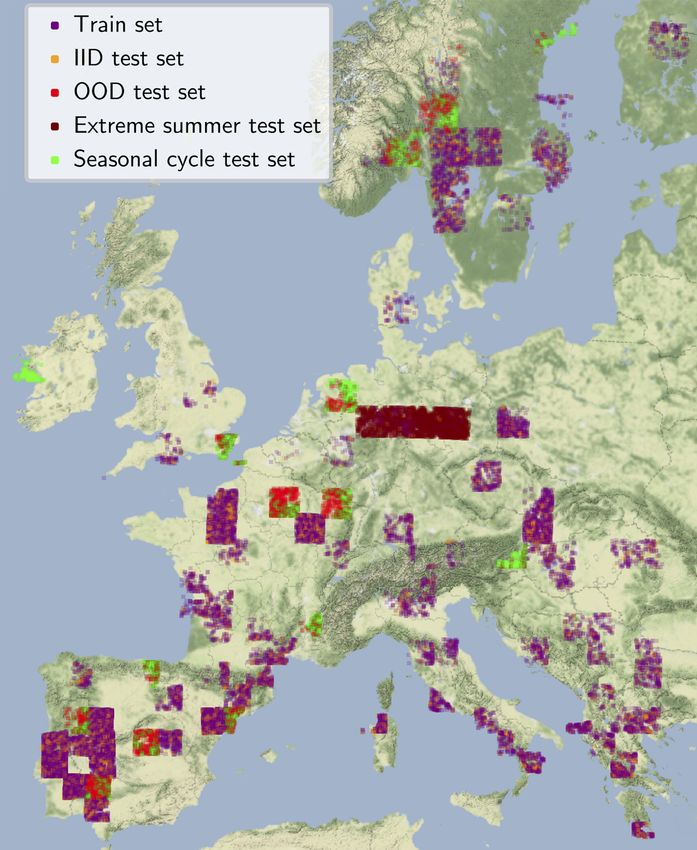
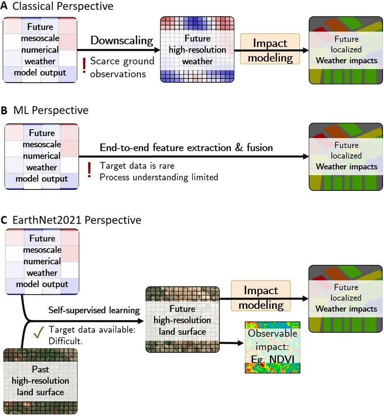
 Figure 1: Overview visualization of one of the over 32000 samples in EarthNet2021.

 Abstract 1. Introduction

 Satellite images are snapshots of the Earth surface. We Seasonal weather forecasts are potentially very valuable
 propose to forecast them. We frame Earth surface forecast- in support of sustainable development goals such as zero
 ing as the task of predicting satellite imagery conditioned hunger or life on land. Spatio-temporal deep learning is ex-
 on future weather. EarthNet2021 is a large dataset suitable pected to improve the predictive ability of seasonal weather
 for training deep neural networks on the task. It contains forecasting [52]. Yet it is unclear, how exactly this expec-
 Sentinel 2 satellite imagery at 20 m resolution, matching tation will materialize. One possible way can be found by
 topography and mesoscale (1.28 km) meteorological vari- carefully thinking about the target variable. The above men-
 ables packaged into 32000 samples. Additionally we frame tioned goals illustrate that ultimately it will not directly be
 EarthNet2021 as a challenge allowing for model intercom- the seasonal meteorological forecasts but rather derived im-
 parison. Resulting forecasts will greatly improve (> ×50) pacts (e.g. agricultural output and ecosystem health) that
 over the spatial resolution found in numerical models. This are of most use to humanity. Such impacts, especially those
 allows localized impacts from extreme weather to be pre- affecting vegetation, materialize on the land surface. Mean-
 dicted, thus supporting downstream applications such as ing, they can be observed on satellite imagery. Thus, high-
 crop yield prediction, forest health assessments or biodi- resolution impact forecasting can be phrased as the pre-
 versity monitoring. Find data, code, and how to participate diction of satellite imagery [15, 24, 29, 38, 73]. Predic-
 at www.earthnet.tech. tion of future frames is also the metier of video prediction
 [2, 22, 37, 43, 46]. Yet, satellite image forecasting can also
 leverage additional future drivers, such as the output of nu-
 * Joint first authors. {crequ,vbenson}@bgc-jena.mpg.de merical weather simulations with earth system models. The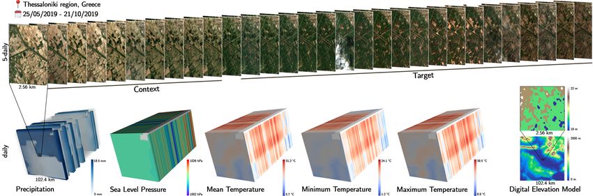

Input Output [53], as well as, the ability to generate stochastic predictions
 Context Guide (future frames) [2, 23, 37], ideal to generate ensemble forecasts of Earth
 surface for effective uncertainty management [72]. Guided
 video prediction is the setting where on top of past frames
Unguided

 {} models have access to future information. We further differ
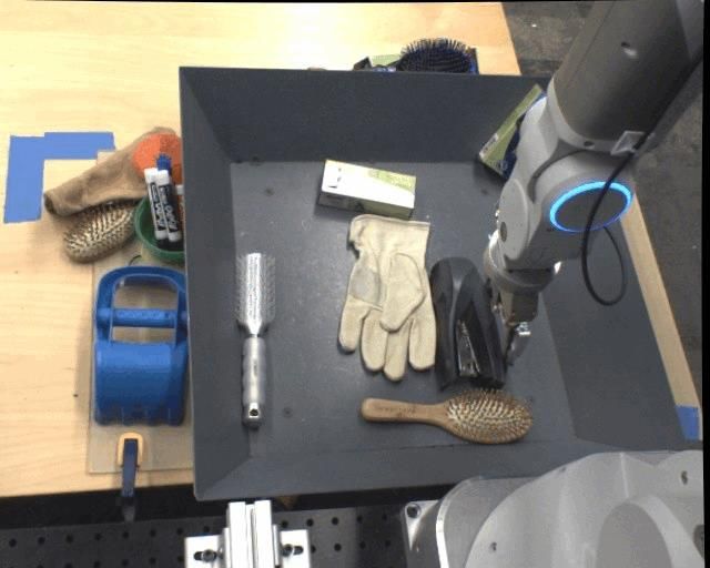
 between weak and strong guiding (Fig. 2). Weakly guided
 models are provided with sparse information of the future,
 for example robot commands [22]. In contrast strongly
Strongly Guided Weakly Guided

 guided models leverage dense spatio-temporal information
 {Robot of the future. This is the setting of EarthNet2021. Some past
 comanded works resemble the strongly guided setting, however either
 poses} the future information are derived from the frames them-
 selves, making the approaches not suitable for prediction
 Dense spatio- [67] or they use the dense spatial information but discard
 temporal drivers the temporal component [42, 53].
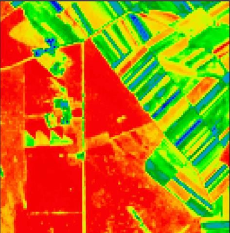
 Modelling weather impact with machine learning. Both
 impact modeling and weather forecasting have been tack-
 led with machine learning methods of different complex-
 ity. One string of literature has focused on forecasting im-
 agery from weather satellites [29, 38, 62, 70] while an-
Figure 2: Video prediction could be unguided, weakly other one has focused on predicting reanalysis data or em-
guided or strongly guided. EarthNet2021 is the first ulating general circulation models [50, 51, 57, 68]. For
dataset specifically designed for the development of spatio- localized weather, statistical downscaling has been lever-
temporal strongly guided video prediction methods. aged [5, 44, 64, 65] (Fig. 3A). Direct impacts of extreme
 weather have been predicted one at a time (Fig. 3B), ex-
general setting of video prediction with additional drivers amples being crop yield [1, 9, 32, 48, 58], vegetation index
is called guided video prediction. We define Earth sur- [15, 26, 49, 69], drought index [47] and soil moisture [19].
face forecasting as the prediction of satellite imagery con-
ditioned on future weather. 3. Motivation
 Our main contributions are summarized as follows: While satellite imagery prediction is an interesting task
 • We motivate the novel task of Earth surface forecast- for video prediction modelers, it is similarly important for
 ing as guided video prediction and define an evaluation domain experts, i.e., climate and land surface scientists. We
 pipeline based the EarthNetScore ranking criterion. focus on predicting localized impacts of extreme weather.
 • We introduce EarthNet2021, a carefully curated large- This is highly relevant since extreme weather impacts very
 scale dataset for Earth surface forecasting conditional heterogeneously at the local scale [34]. Very local factors,
 on meteorological projections. such as vegetation, soil type, terrain elevation or slope, de-
 • We start model intercomparison in Earth surface fore- termine whether a plot is resilient to a heatwave or not. For
 casting with a pilot study encouraging further research example, ecosystems next to a river might survive droughts
 in deep learning video prediction models. more easily than those on south-facing slopes. However, the
 list of all possible spatio-temporal interactions is far from
2. Related work being mechanistically known; hence, it is a source of con-
 siderable amount of uncertainty and an opportunity for pow-
 Earth surface forecasting lays in the intersection of video erful data-driven methods.
prediction and data-driven Earth system modeling. Predicting localized weather impacts can be tackled in
Video prediction. In Fig. 2 we classify video prediction three main ways (Fig. 3). All approaches make use of sea-
tasks into three types depending on the input data used. sonal weather forecasts [8, 10](2 – 6 months ahead). The
Traditionally video prediction models are conditioned on classical approach (Fig. 3A), attempts the hyper-resolution
past context frames and predict future target frames (i.e. of the weather forecast for particular geolocations using sta-
unguided, [17, 18, 22, 25, 31, 36, 40, 43, 60]). The used tistical [7, 66] or dynamical [39] downscaling, that is, corre-
models inherit many characteristics known the be useful in lating the past observed weather with past mesoscale model
modeling Earth surface phenomena: short-long term mem- outputs and using the estimated relationship. The down-
ory effects [35, 55], short-long range spatial relationships scaled weather can then be used in mechanistic models (e.g.

prediction is feasible. Additionally, satellite imagery is also
 used to extract further processed weather impact data prod-
 ucts, such as biodiversity state [21], crop yield [58], soil
 moisture [19] or ground biomass [49]. In short, Earth sur-
 face prediction is promising for forecasting highly localized
 climatic impacts.

 4. EarthNet2021 Dataset
 4.1. Overview

 Data sources. With EarthNet2021 we aim at creating
 the first dataset for the novel task of Earth surface fore-
 casting. The task requires satellite imagery time series at
 high temporal and spatial resolution and additional climatic
 predictors. The two primary public satellite missions for
 high-resolution optical imagery are Landsat and Sentinel 2.
 While the former only revisits each location on Earth ev-
 ery 16 days, the latter does so every five days. Thus we
 choose Sentinel 2 imagery [41] for EarthNet2021. The ad-
 ditional climatic predictors should ideally come from a sea-
 sonal weather model. Obtaining predictions from a global
 seasonal weather model starting at multiple past time steps
Figure 3: Three ways of extreme weather impact predic- is computationally very demanding. Instead, we approx-
tion are A) downscaling meteorological forecasts and sub- imate the forecasts using the E-OBS [14] observational
sequent impact modeling (e.g. runoff models), B) acquiring dataset, which essentially contains interpolated ground truth
target data at high-resolution and using supervised learn- observed weather from a number of stations over Europe.
ing or C) leveraging Earth surface forecasting: This gives This also makes the task easier as uncertain weather fore-
directly obtainable impacts (e.g. NDVI) while still allow- casts are replaced with certain observations. Since E-OBS
ing for impact modeling. Compared to A) and B), large limits the spatial extent to Europe, we use the appropriate
amounts of satellite imagery are available, thus together high-resolution topography: EU-DEM [3].
with self-supervised (i.e. no labeling required) deep learn-
ing large-scale impact prediction becomes feasible. Individual samples. After data processing, EarthNet2021
 contains over 32000 samples, which we call minicubes. A
 single minicube is visualized in Fig. 1. It contains 30 5-
of river discharge) for impact extraction. However, weather daily frames (128 × 128 pixel or 2.56 × 2.56 km) of four
downscaling is a difficult task because it requires ground ob- channels (blue, green, red, near-infrared) of satellite im-
servations from weather stations, which are sparse. A more agery with binary quality masks at high-resolution (20 m),
direct way (Fig. 3B) is to correlate a desired future impact 150 daily frames (80×80 pixel or 102.4×102.4 km) of five
variable, such as crop yields or flood risk, with past data meteorological variables (precipitation, sea level pressure,
(e.g., weather data and vegetation status, [48]). Yet again, mean, minimum and maximum temperature) at mesoscale
this approach requires ground truth data of target variables, resolution (1.28 km) and the static digital elevation model
which is scarce, thus limiting the global applicability of the at both high- and mesoscale resolution. The minicubes re-
approach. veal a strong difference between EarthNet2021 and classic
 Instead, by defining the task of Earth surface forecasting video prediction datasets. In the latter, the objects move in
we propose to use satellite imagery as an intermediate step a 3d space, but images are just a 2d projection of this space.
(Fig. 3C). From satellite imagery, multiple indices describ- For satellite imagery, this effect almost vanishes as the Earth
ing the vegetation state such as the normalized differenced surface locally is very similar to a 2d space.
vegetation index (NDVI) or the enhanced vegetation index 4.2. Generation
(EVI) can be directly observed. These give insights on veg-
etation anomalies, which in turn describe the ecosystem im- Challenges. In general, geospatial datasets are not analysis-
pact at a very local scale. Because of satellite imagery’s ready for standard computer vision. While the former often
vast availability, there is no data scarcity. While technically contain large files together with information about the pro-
difficult, forecasting weather impacts via satellite imagery jection of the data, the latter requires many small data sam-

Sentinel 2 Dataset split
 Metadata-based pre-filtering Quality vs. Bias trade-off
 Subsampling, tile download Iterative sampling process
 Co-registration via arosics Train + 4 test sets

 for each tile: for each cube location:
 Data Fusion Cube generation
 E-OBS climatic variables Creating data quality mask
 EU-DEM surface model Saving compressed array
 Reproject, resample & cut Saving data quality table

Figure 4: The dataset generation scheme of EarthNet2021.

ples on an Euclidean grid. With EarthNet2021 we aim to
bridge the gaps and transform geospatial data into analysis-
ready samples for deep learning. To this end, we had to
gather the satellite imagery, combine it with additional pre-
dictors, generate individual data samples and split these into
training and test sets – challenges which are described in
the following paragraphs and lead to our dataset generation
scheme, see Fig. 4.
Obtaining Sentinel 2 satellite imagery. Downloading the
full archive of Sentinel 2 imagery over Europe would re-
quire downloading Petabytes, rendering the approach un-
feasible. Luckily pre-filtering is possible as the data is split
by the military grid reference system into so-called tiles and
for each tile metadata can be obtained from the AWS Open Figure 5: Spatial distribution of the samples in Earth-
Data Registry1 before downloading. We pre-filter and only Net2021.
download a random subset of 110 tiles with at least 80%
land visible on the least-cloudy day and minimum 90% data cut them to two data windows. The high-resolution win-
coverage. For each tile we download blue, green, red, near- dow has 20 m ground resolution, matching the Sentinel 2
infrared and scene-classification bands over the time series imagery, and the mesoscale window has 1.28 km ground
corresponding to the 5-day interval with the lowest off-nadir resolution.
angle. We use the sentinel-hub library2 to obtain an archive
 Generation of minicubes. Given the fused data, we create
of over 30 TB raw imagery from November 2016 to May
 a target minicube grid, cutting each tile into a regular spatial
2020. In it we notice spatial jittering between consecutive
 grid and a random temporal grid. Spatially, high-resolution
Sentinel 2 intakes, possibly due to the tandem satellites not
 windows of minicube do not overlap, while mesoscale win-
being perfectly co-registered. We try to compensate this ar-
 dows do. Temporally, minicubes at the same location never
tifact by co-registering the time series of each tile. We use
 overlap. For each location in the minicube grid, we extract
the global co-registration from the arosics library3 [56] in-
 the data from our fused archive, generate a data quality (i.e.
side a custom loop.
 cloud) mask based on heuristic rules (similar to [45]) and
Data fusion with E-OBS and EU-DEM. For each of the save the minicube in a compressed numpy array [28]. We
110 tiles we fuse their time series with additional data. also generate data quality indicators; these will be useful for
More particularly we gathered E-OBS4 weather variables selecting cubes during dataset splitting.
(daily mean temperature (T G); daily minimum tempera-
ture (T N ); daily maximum temperature (T X); daily pre-
cipitation sum (RR); and daily averaged sea level pressure Creating the dataset split. In the raw EarthNet2021 corpus
(P P )) at 11.1 km resolution and the EU-DEM5 digital sur- are over 1.3 million minicubes. Unfortunately, most of them
face model at 25 m resolution. We re-project, resample and are of very low quality, mainly because of clouds. Now just
 taking minicubes above a certain quality threshold creates
 1 https://registry.opendata.aws/sentinel-2/
 2 https://sentinelhub-py.readthedocs.io/
 another problem: selection bias. To give an intuitive ex-
 3 https://pypi.org/project/arosics/ ample: most frequently, high-quality (cloud-free) samples
 4 https://surfobs.climate.copernicus.eu/ are found during summer on the Iberian Peninsula, whereas
 5 eea.europa.eu/data-and-maps/data/eu-dem/ there barely are 4 consecutive weeks without clouds on the

British Islands. We address this trade-off by introducing an
iterative filtering process. Until 32000 minicubes are col-
lected, we iteratively loosen quality restrictions for select-
ing high quality cubes and filling them up to obtain balance
among starting months and between northern and southern
geolocations. In a similar random-iterative process we sep-
arate 15 tiles from all downloaded tiles to create a spatial
out-of-domain (OOD) test set (totalling 4214 minicubes)
and randomly split the remainder tiles into 23904 minicubes
for training and 4219 for in-domain (IID) testing.

4.3. Description

Statistics. The EarthNet2021 dataset spans across wider
Central and Western Europe. Its training set contains 23904
samples from 85 regions (Sentinel 2 tiles) in the spatial
extent. Fig. 5 visualizes the spatial distribution of sam-
ples. 71% of the minicubes in the training set lay in the
southern half, which also contains more landmass. In the
northern half we observe a strong clustering in the vicin-
ity of the Oslofjord, which is possibly random. Tempo-
rally most minicubes cover the period of May to October
(Fig. 6a). While this certainly biases the dataset, it might
actually be desirable because some of the most devastating Figure 6: Monthly bias of samples. (a) Shows the monthly
climate impacts (e.g., heatwaves, droughts, wildfires) occur number of minicubes and (b) shows the data quality mea-
during summer. Fig. 6b shows the bias-quality trade-off, sured by the percentage of masked (mainly cloudy) pixels
observe that most high quality minicubes are from summer over both, months and latitude.
in the Mediterranean. Also, it shows that EarthNet2021
does not contain samples covering winter in the northern
latitudes. This is possibly an effect of our very restrictive
quality masking wrongly classifying snow as clouds. 5. EarthNet2021 Challenge
Comparison to other datasets. Earth surface forecasting is
 5.1. Overview
a novel task, thus there are no such datasets prior to Earth-
Net2021. Still, since it also belongs to the broader set of
 Model intercomparison. Modeling efforts are most use-
analysis-ready datasets for deep learning, we can assert that
 ful when different models can easily be compared. Then,
it is large enough for training deep neural networks. In sup-
 strengths and weaknesses of different approaches can be
plementary table 2 we compare a range of datasets using ei-
 identified and state-of-the-art methods selected. We pro-
ther satellite imagery or being targeted to video prediction
 pose the EarthNet2021 challenge as a model intercompar-
models. By pure sample size, EarthNet2021 ranks solid,
 ison exercise in Earth surface forecasting built on top of
yet, the number is misleading since individual samples are
 the EarthNet2021 dataset. This motivation is reflected in
different. By additionally comparing the size in gigabytes,
 the design of the challenge. We define an evaluation proto-
we assert that EarthNet2021 is indeed a large dataset.
 col by which approaches can be compared as well as pro-
Limitations. Clearly, EarthNet2021 limits models to work vide a framework, such that knowledge between modelers
solely on Earth surface forecasting in Europe. Additionally, is easily exchanged. There is no reward other than scien-
the dataset is subject to a selection bias; therefore, there are tific contribution and a publicly visible leaderboard. Eval-
areas in Europe for which model generalizability could be uating Earth surface forecasts is not trivial. Since it is a
problematic. Furthermore, EarthNet2021 leverages obser- new task, there is not yet a commonly used criterion. We
vational products instead of actual forecasts. Thus, while design the EarthNetScore as a ranking criterion balancing
this certainly is practical for a number of reasons, Earth sur- multiple goals and center the evaluation pipeline around it
face models trained on EarthNet2021 should be viewed as (see Fig. 7). Moreover, we motivate four challenge tracks.
experimental and might not be plug-and-play into produc- These allow comparison of models’ validity and robustness
tion with seasonal weather model forecasts. and applicability to extreme events and the vegetation cycle.

are also largely robust to missing data points, which poses a
 consistency constraint on model predictions at output pixels
 ! compute
 output
 EarthNetScore for which no target data is available. Finally, the structural
 on non-masked pixels
 similarity index SSIM is a perceptual metric imposing pre-
 inputs
 Machine Ground truth

 Learning & mask Pick best sample dicted frames to have similar spatial structure to the target
 per multicube satellite images. All component scores are modified to work
 Model
 " Aggregate over
 properly in the presence of a data quality mask, rescaled to
 ... full dataset
 match difficulty and transformed to lay between 0 (worst)
 and 1 (best).
 Ensemble of Model performance:
 10 predictions EarthNetScore Computation. Combining these components is another
Challenge tracks: Extreme summer Seasonal cycle
IID ! = 10 | " = 20 ! = 20 | " = 40 ! = 70 | " = 140
 challenge. We would like to define the EarthNetScore as:
OOD ! = 10 | " = 20 Feb – May | June – Nov 2017 – 2018 | 2018 – 2020
 4
Figure 7: Evaluation pipeline for models on EarthNet2021. EN S = 1 1 1 1 . (1)
 ( M AD + OLS + EM D + SSIM )
For predicting the tT target frames, a model can use satel-
lite images from the tC context frames, the static DEM and This is the harmonic mean of the four components, so it
mesoscale climatic variables including those from the target lays strongly to the worst performing component. Yet, com-
time steps. puting EN S over a full test set requires further clarifica-
 tion. Earth surface forecasting is a stochastic prediction
EarthNet2021 framework. To facilitate research we pro-
 task, models are allowed to output an ensemble of predic-
vide a flexible framework which kick-starts modelers and
 tions. Thus, for each minicube in the test set there might
removes double work between groups. The evaluation
 multiple predictions (up to 10). In line with what is com-
pipeline is packaged in the EarthNet2021 toolkit and lever-
 monly done in video prediction, we compute the subscores
ages multiprocessing for fast inference. Additionally, chal-
 for each one of them but, only take the prediction for which
lenge participants are encouraged to use the model inter-
 equation 1 is highest for model intercomparison. In other
comparison suite. It shall give one entry point for running
 words, the evaluation pipeline only accounts for the best
a wide range of models. Currently it features model tem-
 prediction per minicube. This is superior to average predic-
plates in PyTorch and TensorFlow and additional graphical
 tions as it allows for an ensemble of discrete, sharp, plausi-
output useful for debugging and visual comparison.
 ble outcomes, something desired for Earth surface forecast-
 ing given its highly multimodal nature. Still, this evaluation
 scheme, suffers severely from not being able to rank models
5.2. EarthNetScore according to their modeled distribution. Once the compo-
 nents for the best predictions for all minicubes in the dataset
Components. Evaluating Earth surface predictions is non- are collected, we average each component and then calcu-
trivial. Firstly, because the topological space of spectral im- late the EN S by feeding the averages to equation 1. Then,
ages is not a metric space, secondly, because clouds and the EN S ranges from 0 to 1, where 1 is a perfect prediction.
other data degradation hinder evaluation, and, thirdly, be-
cause ranking simply by root mean squared error might 5.3. Tracks
lead to ordinal rankings of imperfect predictions that ex-
perts would not agree to. Instead of using a single score, Main (IID) track. The EarthNet2021 main track checks
we define the EarthNetScore EN S by combining multiple model validity. It uses the IID test set, which has minicubes
components. As the first component, we use the median ab- that are very similar (yet randomly split) as those seen dur-
solute deviation M AD. It is a robust distance in pixel-space ing training. Models get 10 context frames of high res-
which is justified by the goal that predicted and target values olution 5-daily multispectral satellite imagery (time [t-45,
should be close. Secondly, OLS, the difference of ordinary t]), static topography at both mesoscale and high resolu-
least squares linear regression slopes of pixelwise Normal- tion, and mesoscale dynamic climate conditions for 150
ized Difference Vegetation Index (NDVI) timeseries, gives past and future days (time [t-50, t+100]). Models shall
an indicator as to whether the predictions are able to repro- output 20 frames of high-resolution sentinel 2 bands red,
duce the trend in vegetation change. This together with the green, blue and near-infrared for the next 100 days (time
Earth mover distance EM D between pixelwise NDVI time [t+5,t+100]). These predictions are then evaluated with the
series over the short span of 20 time steps is a good proxy EarthNetScore on cloud-free pixels from the ground truth.
of the fit (in the distribution and direction) of the vegetation This track follows the assumption that, in production, any
time series. The time series based metrics OLS and EM D Earth surface forecasting model would have access to all

IID OOD
 ENS MAD OLS EMD SSIM ENS MAD OLS EMD SSIM
 Persistence 0.2625 0.2315 0.3239 0.2099 0.3265 0.2587 0.2248 0.3236 0.2123 0.3112
 Channel-U-Net 0.2902 0.2482 0.3381 0.2336 0.3973 0.2854 0.2402 0.3390 0.2371 0.3721
 Arcon 0.2803 0.2414 0.3216 0.2258 0.3863 0.2655 0.2314 0.3088 0.2177 0.3432

 Table 1: Models performance on EarthNet2021. See supplementary material for Extreme and Seasonal test sets.

prior Earth observation data, thus the test set has the same 6. Models
underlying distribution as the training set.
 As first baselines in the EarthNet2021 model intercom-
 parison, we provide three models. One is a naive averaging
Robustness (OOD) track. In addition to the main track, persistence baseline while the other two are deep learning
we offer a robustness track. Even on the same satellite data, models slightly modified for guided video prediction. Per-
deep learning models might generalize poorly across geolo- formance is reported in Tab. 1.
cations [6], thus it is important to check model performance
on an out-of-domain (OOD) test set. This track has a weak Persistence baseline The EarthNet2021 unified toolkit
OOD setting; in which minicubes solely are from differ- comes with a pre-implemented baseline in NumPy. It sim-
ent Sentinel 2 tiles than those seen during training, which ply averages cloud-free pixels over the context frames and
is possibly only a light domain shift. Still, it is useful as a uses that value as a constant prediction. Performance is
first benchmark to check applicability of models outside the shown in table 1.
training domain. Autorregressive Conditional video prediction baseline
 The Autorregressive Conditional video prediction baseline
 (Arcon) is based on Stochastic adversarial video prediction
Extreme summer track. Furthermore, EarthNet2021 con-
 (SAVP, [37]) that was originally was used as an unguided
tains two tracks particularly focused on Earth system sci-
 or weakly guided video prediction model. We extend SAVP
ence hot topics, which should both be understood as more
 for EarthNet2021 by stacking the guiding variables as extra
experimental. The extreme summer track contains cubes
 video channels. To this end, climatic variables had to be
from the extreme summer 2018 in northern Germany [4],
 resampled to match imagery resolution. In addition, SAVP
with 4 months of context (20 frames) starting from Febru-
 cannot make use of the different temporal resolution of pre-
ary and 6 months (40 frames) starting from June to evaluate
 dictors and targets (daily vs. 5 daily) so predictors were
predictions. For these locations, only cubes before 2018
 reduced by taking the 5-daily mean, these steps resulted in
are in the training set. Being able to accurately downscale
 guiding information loss. Since there is no moving objects
the prediction of an extreme heat event and to predict the
 in satellite imagery, but just a widely variable background,
vegetation response at a local scale would greatly benefit
 all SAVP components specifically designed for motion pre-
research on resilience strategies. In addition, the extreme
 diction were disabled. Image generation from scratch and
summer track can in some sense be understood as a tempo-
 reuse of context frames as background was enabled. Dif-
ral OOD setting.
 ferent to traditional video input data, EarthNet2021 input
 satellite imagery is defective, as a model shall not forecast
Seasonal cycle track. While not the focus of Earth- clouds and other artifacts. Thus, different to the original im-
Net2021, models are likely able to generate predictions for plementation, we train Arcon just with mean absolute error
longer horizons. Thus, we include the seasonal cycle track over non-masked pixels; in particular, this means no adver-
covering multiple years of observations; hence, including sarial loss was used.
vegetation full seasonal cycle. This track is also in line Arcon outperforms the persistence baseline in every test
with the recently rising interest in seasonal forecasts within set except the full seasonal cycle test (see table 1 for IID
physical climate models. It contains minicubes from the and OOD results), where, possibly the model breaks down
spatial OOD setting also used for the robustness tracks, but when fed a context length higher than 10. The model shows
this time each minicube comes with 1 year (70 frames) of degrading forecasting performance at the longer temporal
context frames and 2 years (140 frames) to evaluate pre- horizon (see Fig. 8). These results give us two hints. First,
dictions. For this longer prediction length, we change the it is necessary to overhaul and adapt current video predic-
EarthNetScore OLS component to be calculated over dis- tion models to make them capable of tackling the strongly
joint windows of 20 frames each. guided setting. Second, since the slightly adapted SAVP

Context Prediction Channel-U-Net is the overall best performing model,
 t=5 t=10 t=11 t=15 t=20 t=25 t=30
 even though it does not model temporal dependencies ex-
 plicitly. This model also underperforms the persistence
 Arcon

 baseline on the seasonal test set, possibly due to the slid-
Worst

 ing window approach used for the much longer prediction
 length.
 GT

 7. Outlook
 Arcon
Median

 If solved, Earth surface forecasting will greatly benefit
 society by providing seasonal predictions of climate im-
 GT

 pacts at a local scale. These are extremely informative
 for implementing preventive mitigation strategies. Earth-
 Arcon

 Net2021 is a stepping-stone towards the collaboration that
Best

 is necessary between modelers from Computer Vision and
 domain experts from the Earth System Sciences. The
 GT

 dataset requires developing guided video prediction mod-
 els, a unique opportunity for video prediction researchers
Figure 8: Worst, median and best samples predicted by Ar- to extend their approaches. Since the guided setting allows
con according to EarthNetScore over the full IID test set. modeling in a more controlled environment, there is the pos-
Yellow line marks the beginning of the predicted frames. sibility, that gained knowledge can also be transferred back
 to general (unguided) video prediction. Eventually, numer-
shows skill over the persistence baseline, we can anticipate ical Earth System Models [20] could benefit from the data-
current video prediction models to be a useful starting point. driven high-resolution modelling by Earth surface forecast-
 ing models. In so-called hybrid models [52], both compo-
Channel-U-Net baseline nents could be combined.
 This architecture is inspired by the winning solution to EarthNet2021 is the first dataset for spatio-temporal
the 2020 Traffic4cast challenge [12]. Traffic map forecast- Earth surface forecasting. As such, it comes with a num-
ing is to a certain degree similar to the proposed task of ber of limitations, including some that will be discovered
Earth surface forecasting. The solution used a U-Net ar- during model development. Through the EarthNet2021
chitecture [54] with dense connections between layers. All framework, especially the model intercomparison suite, we
available context time step inputs were stacked along the hope to create a space for communication between differ-
channel dimension and fed into the network. Subsequently ent stakeholders. Then, we could remove pressing issues
the model outputs all future time steps stacked along the iteratively. We hope EarthNet2021 will serve as a starting
channel dimension, which are then reshaped for proper point for community building around high-resolution Earth
evaluation. We call such an approach a Channel-U-Net. surface forecasting.
Here we present a Channel-U-Net with an ImageNet [16]
pre-trained DenseNet161 [30] encoder from the Segmenta- Acknowledgements We thank three anonymous reviewers and the
tion Models PyTorch library6 . As inputs we feed the center area chair for their constructive reviews. We are grateful to the
2x2 meteorological predictors upsampled to full spatial res- Centre for Information Services and High Performance Comput-
olution, the high-resolution DEM and all the satellite chan- ing [Zentrum für Informationsdienste und Hochleistungsrechnen
nels from the 10 context time steps, resulting in 191 input (ZIH)] TU Dresden for providing its facilities for high throughput
channels. The model outputs 80 channels activated with a calculations.
sigmoid, corresponding to the four color channels for each Authors contribution C.R. Experimental design, EarthNet model
of the 20 target time steps. We trained the model for 100 intercomparison suite, baseline persistence and Arcon models,
 website, documentation, manuscript. V.B. Experimental de-
Epochs on a quality masked L1 loss with Adam [33], an
 sign, dataset creation pipeline, EarthNet toolkit package, baseline
initial learning rate of 0.002, decreased by a factor 10 after channel-net model, website, documentation, manuscript. M.R.
40, 70 and 90 epochs. We use a batch size of 64 and 4 x Experimental design, metric selection, manuscript revision. J.R.
V100 16GB GPUs. For the extreme and the seasonal tracks Experimental design, manuscript revision. J.D. Experimental de-
we slide the model through the time series by feeding back sign, metric selection, manuscript revision.
its previous outputs as new inputs after the initial prediction, Code and data availability All information is provided on our
which uses the last 10 frames of context available. website www.earthnet.tech.
 6 https://smp.readthedocs.io/

References Conference on Computer Vision and Pattern Recognition,
 pages 2828–2838, 2020.
 [1] Khalid A Al-Gaadi, Abdalhaleem A Hassaballa, ElKamil [12] Sungbin Choi. Utilizing unet for the future traffic map
 Tola, Ahmed G Kayad, Rangaswamy Madugundu, Ban- prediction task traffic4cast challenge 2020. arXiv preprint
 der Alblewi, and Fahad Assiri. Prediction of potato crop arXiv:2012.00125, 2020.
 yield using precision agriculture techniques. PloS one,
 [13] Marius Cordts, Mohamed Omran, Sebastian Ramos, Timo
 11(9):e0162219, 2016.
 Rehfeld, Markus Enzweiler, Rodrigo Benenson, Uwe
 [2] Mohammad Babaeizadeh, Chelsea Finn, Dumitru Erhan, Franke, Stefan Roth, and Bernt Schiele. The cityscapes
 Roy H Campbell, and Sergey Levine. Stochastic variational dataset for semantic urban scene understanding. In Proceed-
 video prediction. arXiv preprint arXiv:1710.11252, 2017. ings of the IEEE conference on computer vision and pattern
 [3] A Bashfield and A Keim. Continent-wide dem creation for recognition, pages 3213–3223, 2016.
 the european union. In 34th International Symposium on Re- [14] Richard Cornes, Gerard van der Schrier, Else van den Besse-
 mote Sensing of Environment. The GEOSS Era: Towards laar, and Philip Jones. An ensemble version of the e-obs tem-
 Operational Environmental Monitoring. Sydney, Australia, perature and precipitation data sets. Journal of Geophysical
 pages 10–15, 2011. Research: Atmospheres, 123(17):9391–9409, 2018.
 [4] Ana Bastos, P Ciais, P Friedlingstein, S Sitch, Julia Pongratz, [15] Monidipa Das and Soumya K Ghosh. Deep-step: A deep
 L Fan, JP Wigneron, Ulrich Weber, Markus Reichstein, Z learning approach for spatiotemporal prediction of remote
 Fu, et al. Direct and seasonal legacy effects of the 2018 heat sensing data. IEEE Geoscience and Remote Sensing Letters,
 wave and drought on european ecosystem productivity. Sci- 13(12):1984–1988, 2016.
 ence advances, 6(24):eaba2724, 2020. [16] Jia Deng, Wei Dong, Richard Socher, Li-Jia Li, Kai Li,
 [5] Joaquı́n Bedia, Jorge Baño-Medina, Mikel N Legasa, Ma- and Li Fei-Fei. Imagenet: A large-scale hierarchical image
 ialen Iturbide, Rodrigo Manzanas, Sixto Herrera, Ana database. In 2009 IEEE conference on computer vision and
 Casanueva, Daniel San-Martı́n, Antonio S Cofiño, and pattern recognition, pages 248–255. Ieee, 2009.
 José Manuel Gutiérrez. Statistical downscaling with the [17] Emily L Denton et al. Unsupervised learning of disentangled
 downscaler package (v3. 1.0): contribution to the value inter- representations from video. In Advances in neural informa-
 comparison experiment. Geoscientific Model Development, tion processing systems, pages 4414–4423, 2017.
 13(3), 2020. [18] Frederik Ebert, Chelsea Finn, Alex X. Lee, and Sergey
 [6] Vitus Benson and Alexander Ecker. Assessing out-of- Levine. Self-supervised visual planning with temporal skip
 domain generalization for robust building damage detec- connections, 2017.
 tion. AI for Humanitarian Assistance and Disaster Response [19] Natalia Efremova, Dmitry Zausaev, and Gleb Antipov. Pre-
 workshop (NeurIPS 2020), 2020. diction of soil moisture content based on satellite data and
 [7] J Boé, L Terray, F Habets, and E Martin. A simple statistical- sequence-to-sequence networks. NeurIPS 2018 Women in
 dynamical downscaling scheme based on weather types and Machine Learning workshop, 2019.
 conditional resampling. Journal of Geophysical Research: [20] Veronika Eyring, Sandrine Bony, Gerald A Meehl, Cather-
 Atmospheres, 111(D23), 2006. ine A Senior, Bjorn Stevens, Ronald J Stouffer, and Karl E
 [8] Gilbert Brunet, Melvyn Shapiro, Brian Hoskins, Mitch Mon- Taylor. Overview of the coupled model intercomparison
 crieff, Randall Dole, George N Kiladis, Ben Kirtman, An- project phase 6 (cmip6) experimental design and organiza-
 drew Lorenc, Brian Mills, Rebecca Morss, et al. Collab- tion. Geoscientific Model Development, 9(5):1937–1958,
 oration of the weather and climate communities to advance 2016.
 subseasonal-to-seasonal prediction. Bulletin of the American [21] Mathieu Fauvel, Mailys Lopes, Titouan Dubo, Justine
 Meteorological Society, 91(10):1397–1406, 2010. Rivers-Moore, Pierre-Louis Frison, Nicolas Gross, and An-
 [9] Yaping Cai, Kaiyu Guan, David Lobell, Andries B Potgieter, nie Ouin. Prediction of plant diversity in grasslands using
 Shaowen Wang, Jian Peng, Tianfang Xu, Senthold Asseng, sentinel-1 and-2 satellite image time series. Remote Sensing
 Yongguang Zhang, Liangzhi You, et al. Integrating satel- of Environment, 237:111536, 2020.
 lite and climate data to predict wheat yield in australia using [22] Chelsea Finn, Ian Goodfellow, and Sergey Levine. Unsuper-
 machine learning approaches. Agricultural and forest mete- vised learning for physical interaction through video predic-
 orology, 274:144–159, 2019. tion. arXiv preprint arXiv:1605.07157, 2016.
[10] Pierre Cantelaube and Jean-Michel Terres. Seasonal weather [23] Jean-Yves Franceschi, Edouard Delasalles, Mickaël Chen,
 forecasts for crop yield modelling in europe. Tellus A: Sylvain Lamprier, and Patrick Gallinari. Stochastic latent
 Dynamic Meteorology and Oceanography, 57(3):476–487, residual video prediction. In International Conference on
 2005. Machine Learning, pages 3233–3246. PMLR, 2020.
[11] Mang Tik Chiu, Xingqian Xu, Yunchao Wei, Zilong Huang, [24] Feng Gao, Jeff Masek, Matt Schwaller, and Forrest Hall. On
 Alexander G Schwing, Robert Brunner, Hrant Khacha- the blending of the landsat and modis surface reflectance:
 trian, Hovnatan Karapetyan, Ivan Dozier, Greg Rose, et al. Predicting daily landsat surface reflectance. IEEE Transac-
 Agriculture-vision: A large aerial image database for agri- tions on Geoscience and Remote sensing, 44(8):2207–2218,
 cultural pattern analysis. In Proceedings of the IEEE/CVF 2006.

[25] Hang Gao, Huazhe Xu, Qi-Zhi Cai, Ruth Wang, Fisher Yu, [37] Alex X Lee, Richard Zhang, Frederik Ebert, Pieter Abbeel,
 and Trevor Darrell. Disentangling propagation and genera- Chelsea Finn, and Sergey Levine. Stochastic adversarial
 tion for video prediction. In Proceedings of the IEEE/CVF video prediction. arXiv preprint arXiv:1804.01523, 2018.
 International Conference on Computer Vision (ICCV), Octo- [38] Jae-Hyeok Lee, Sangmin S Lee, Hak Gu Kim, Sa-Kwang
 ber 2019. Song, Seongchan Kim, and Yong Man Ro. Mcsip net:
[26] Andrea Gobbi, Marco Cristoforetti, Giuseppe Jurman, and Multichannel satellite image prediction via deep neural net-
 Cesare Furlanello. High resolution forecasting of heat waves work. IEEE Transactions on Geoscience and Remote Sens-
 impacts on leaf area index by multiscale multitemporal deep ing, 58(3):2212–2224, 2019.
 learning. arXiv preprint arXiv:1909.07786, 2019. [39] Jeff Chun-Fung Lo, Zong-Liang Yang, and Roger A
[27] Ritwik Gupta, Bryce Goodman, Nirav Patel, Ricky Hosfelt, Pielke Sr. Assessment of three dynamical climate down-
 Sandra Sajeev, Eric Heim, Jigar Doshi, Keane Lucas, Howie scaling methods using the weather research and forecast-
 Choset, and Matthew Gaston. Creating xbd: A dataset for ing (wrf) model. Journal of Geophysical Research: Atmo-
 assessing building damage from satellite imagery. In Pro- spheres, 113(D9), 2008.
 ceedings of the IEEE Conference on Computer Vision and [40] William Lotter, Gabriel Kreiman, and David Cox. Deep pre-
 Pattern Recognition Workshops, pages 10–17, 2019. dictive coding networks for video prediction and unsuper-
[28] Charles R Harris, K Jarrod Millman, Stéfan J van der vised learning. arXiv preprint arXiv:1605.08104, 2016.
 Walt, Ralf Gommers, Pauli Virtanen, David Cournapeau, [41] Jérôme Louis, Vincent Debaecker, Bringfried Pflug, Mag-
 Eric Wieser, Julian Taylor, Sebastian Berg, Nathaniel J dalena Main-Knorn, Jakub Bieniarz, Uwe Mueller-Wilm,
 Smith, et al. Array programming with numpy. Nature, Enrico Cadau, and Ferran Gascon. Sentinel-2 sen2cor: L2a
 585(7825):357–362, 2020. processor for users. In Proceedings Living Planet Sympo-
 sium 2016, pages 1–8. Spacebooks Online, 2016.
[29] Seungkyun Hong, Seongchan Kim, Minsu Joh, and Sa-
 Kwang Song. Psique: Next sequence prediction of satellite [42] Björn Lütjens, Brandon Leshchinskiy, Christian Requena-
 images using a convolutional sequence-to-sequence network. Mesa, Farrukh Chishtie, Natalia Dı́az-Rodriguez, Océane
 Workshop on Deep Learning for Physical Sciences (NeurIPS Boulais, Aaron Piña, Dava Newman, Alexander Lavin, Yarin
 2017), 2017. Gal, et al. Physics-informed gans for coastal flood visualiza-
 tion. arXiv preprint arXiv:2010.08103, 2020.
[30] Forrest Iandola, Matt Moskewicz, Sergey Karayev, Ross Gir-
 shick, Trevor Darrell, and Kurt Keutzer. Densenet: Im- [43] Michael Mathieu, Camille Couprie, and Yann LeCun. Deep
 plementing efficient convnet descriptor pyramids. arXiv multi-scale video prediction beyond mean square error.
 preprint arXiv:1404.1869, 2014. arXiv preprint arXiv:1511.05440, 2015.
 [44] Jorge Baño Medina, José Manuel Gutiérrez, and Sixto Her-
[31] Nal Kalchbrenner, Aäron Oord, Karen Simonyan, Ivo Dani-
 rera Garcı́a. Deep neural networks for statistical downscal-
 helka, Oriol Vinyals, Alex Graves, and Koray Kavukcuoglu.
 ing of climate change projections. In XVIII Conferencia de la
 Video pixel networks. In International Conference on Ma-
 Asociación Española para la Inteligencia Artificial (CAEPIA
 chine Learning, pages 1771–1779. PMLR, 2017.
 2018) 23-26 de octubre de 2018 Granada, España, pages
[32] Elisa Kamir, François Waldner, and Zvi Hochman. Estimat- 1419–1424. Asociación Española para la Inteligencia Artifi-
 ing wheat yields in australia using climate records, satellite cial (AEPIA), 2018.
 image time series and machine learning methods. ISPRS
 [45] Andrea Meraner, Patrick Ebel, Xiao Xiang Zhu, and Michael
 Journal of Photogrammetry and Remote Sensing, 160:124–
 Schmitt. Cloud removal in sentinel-2 imagery using a deep
 135, 2020.
 residual neural network and sar-optical data fusion. ISPRS
[33] Diederik P Kingma and Jimmy Ba. Adam: A method for Journal of Photogrammetry and Remote Sensing, 166:333–
 stochastic optimization. arXiv preprint arXiv:1412.6980, 346, 2020.
 2014. [46] Junhyuk Oh, Xiaoxiao Guo, Honglak Lee, Richard L Lewis,
[34] Felix N Kogan. Remote sensing of weather impacts on veg- and Satinder Singh. Action-conditional video prediction us-
 etation in non-homogeneous areas. International Journal of ing deep networks in atari games. In Advances in neural
 remote sensing, 11(8):1405–1419, 1990. information processing systems, pages 2863–2871, 2015.
[35] Basil Kraft, Martin Jung, Marco Körner, Christian Re- [47] Haekyung Park, Kyungmin Kim, et al. Prediction of severe
 quena Mesa, José Cortés, and Markus Reichstein. Identi- drought area based on random forest: Using satellite image
 fying dynamic memory effects on vegetation state using re- and topography data. Water, 11(4):705, 2019.
 current neural networks. Frontiers in Big Data, 2, 2019. [48] Bin Peng, Kaiyu Guan, Ming Pan, and Yan Li. Benefits of
[36] David P Kreil, Michael K Kopp, David Jonietz, Moritz Neun, seasonal climate prediction and satellite data for forecasting
 Aleksandra Gruca, Pedro Herruzo, Henry Martin, Ali So- us maize yield. Geophysical Research Letters, 45(18):9662–
 leymani, and Sepp Hochreiter. The surprising efficiency of 9671, 2018.
 framing geo-spatial time series forecasting as a video pre- [49] Pierre Ploton, Nicolas Barbier, Pierre Couteron, CM Antin,
 diction task–insights from the iarai traffic4cast competition Narayanan Ayyappan, N Balachandran, N Barathan, J-F
 at neurips 2019. In NeurIPS 2019 Competition and Demon- Bastin, G Chuyong, Gilles Dauby, et al. Toward a general
 stration Track, pages 232–241. PMLR, 2020. tropical forest biomass prediction model from very high res-

olution optical satellite images. Remote sensing of environ- [62] Pham Huy Thong et al. Some novel hybrid forecast meth-
 ment, 200:140–153, 2017. ods based on picture fuzzy clustering for weather nowcast-
[50] Stephan Rasp, Peter D Dueben, Sebastian Scher, Jonathan A ing from satellite image sequences. Applied Intelligence,
 Weyn, Soukayna Mouatadid, and Nils Thuerey. Weather- 46(1):1–15, 2017.
 bench: A benchmark data set for data-driven weather fore- [63] Adam Van Etten, Dave Lindenbaum, and Todd M Bacastow.
 casting. Journal of Advances in Modeling Earth Systems, Spacenet: A remote sensing dataset and challenge series.
 12(11):e2020MS002203, 2020. arXiv preprint arXiv:1807.01232, 2018.
[51] Stephan Rasp and Nils Thuerey. Data-driven medium-range [64] Thomas Vandal, Evan Kodra, Sangram Ganguly, Andrew
 weather prediction with a resnet pretrained on climate simu- Michaelis, Ramakrishna Nemani, and Auroop R Ganguly.
 lations: A new model for weatherbench. Journal of Advances Deepsd: Generating high resolution climate change projec-
 in Modeling Earth Systems, 13(2):e2020MS002405, 2021. tions through single image super-resolution. In Proceedings
[52] Markus Reichstein, Gustau Camps-Valls, Bjorn Stevens, of the 23rd acm sigkdd international conference on knowl-
 Martin Jung, Joachim Denzler, Nuno Carvalhais, and Prab- edge discovery and data mining, pages 1663–1672, 2017.
 hat. Deep learning and process understanding for data-driven [65] Thomas Vandal, Evan Kodra, Sangram Ganguly, Andrew
 earth system science. Nature, 566(7743):195–204, 2019. Michaelis, Ramakrishna Nemani, and Auroop R Gan-
[53] Christian Requena-Mesa, Markus Reichstein, Miguel Ma- guly. Generating high resolution climate change projections
 hecha, Basil Kraft, and Joachim Denzler. Predicting land- through single image super-resolution: An abridged version.
 scapes from environmental conditions using generative net- In International Joint Conferences on Artificial Intelligence
 works. In German Conference on Pattern Recognition, pages Organization, 2018.
 203–217. Springer, 2019.
 [66] Mathieu Vrac, Michael Stein, and Katharine Hayhoe. Statis-
[54] Olaf Ronneberger, Philipp Fischer, and Thomas Brox. U- tical downscaling of precipitation through nonhomogeneous
 net: Convolutional networks for biomedical image segmen- stochastic weather typing. Climate Research, 34(3):169–
 tation. In International Conference on Medical image com- 184, 2007.
 puting and computer-assisted intervention, pages 234–241.
 [67] Ting-Chun Wang, Ming-Yu Liu, Jun-Yan Zhu, Guilin Liu,
 Springer, 2015.
 Andrew Tao, Jan Kautz, and Bryan Catanzaro. Video-to-
[55] Marc Rußwurm and Marco Korner. Temporal vegetation
 video synthesis. arXiv preprint arXiv:1808.06601, 2018.
 modelling using long short-term memory networks for crop
 identification from medium-resolution multi-spectral satel- [68] Jonathan A Weyn, Dale R Durran, and Rich Caru-
 lite images. In Proceedings of the IEEE Conference on Com- ana. Improving data-driven global weather prediction
 puter Vision and Pattern Recognition Workshops, pages 11– using deep convolutional neural networks on a cubed
 19, 2017. sphere. Journal of Advances in Modeling Earth Systems,
[56] Daniel Scheffler, André Hollstein, Hannes Diedrich, Karl 12(9):e2020MS002109, 2020.
 Segl, and Patrick Hostert. Arosics: An automated and robust [69] Aleksandra Wolanin, Gustau Camps-Valls, Luis Gómez-
 open-source image co-registration software for multi-sensor Chova, Gonzalo Mateo-Garcı́a, Christiaan van der Tol,
 satellite data. Remote Sensing, 9(7):676, 2017. Yongguang Zhang, and Luis Guanter. Estimating crop pri-
[57] Sebastian Scher and Gabriele Messori. Weather and climate mary productivity with sentinel-2 and landsat 8 using ma-
 forecasting with neural networks: using general circulation chine learning methods trained with radiative transfer sim-
 models (gcms) with different complexity as a study ground. ulations. Remote Sensing of Environment, 225:441–457,
 Geoscientific Model Development, 12(7):2797–2809, 2019. 2019.
[58] Raı́ A Schwalbert, Telmo Amado, Geomar Corassa, [70] Zhan Xu, Jun Du, Jingjing Wang, Chunxiao Jiang, and Yong
 Luan Pierre Pott, PV Vara Prasad, and Ignacio A Ciampitti. Ren. Satellite image prediction relying on gan and lstm neu-
 Satellite-based soybean yield forecast: Integrating machine ral networks. In ICC 2019-2019 IEEE International Confer-
 learning and weather data for improving crop yield predic- ence on Communications (ICC), pages 1–6. IEEE, 2019.
 tion in southern brazil. Agricultural and Forest Meteorology, [71] Xiaoxiang Zhu, Chunping Qiu, Jingliang Hu, Andrés
 284:107886, 2020. Camero Unzueta, Lukas Kondmann, Aysim Toker, Gio-
[59] Khurram Soomro, Amir Roshan Zamir, and Mubarak Shah. vanni Marchisio, and Laura Leal-Taixé. Dynamicearth-
 Ucf101: A dataset of 101 human actions classes from videos net challenge at earthvision 2021, http://www.classic.grss-
 in the wild. arXiv preprint arXiv:1212.0402, 2012. ieee.org/earthvision2021/challenge.html.
[60] Nitish Srivastava, Elman Mansimov, and Ruslan Salakhudi- [72] Yuejian Zhu. Ensemble forecast: A new approach to uncer-
 nov. Unsupervised learning of video representations using tainty and predictability. Advances in atmospheric sciences,
 lstms. In International conference on machine learning, 22(6):781–788, 2005.
 pages 843–852, 2015. [73] Zhe Zhu, Curtis E Woodcock, Christopher Holden, and
[61] Gencer Sumbul, Marcela Charfuelan, Begüm Demir, and Zhiqiang Yang. Generating synthetic landsat images based
 Volker Markl. Bigearthnet: A large-scale benchmark archive on all available landsat data: Predicting landsat surface re-
 for remote sensing image understanding. In IGARSS 2019- flectance at any given time. Remote Sensing of Environment,
 2019 IEEE International Geoscience and Remote Sensing 162:67–83, 2015.
 Symposium, pages 5901–5904. IEEE, 2019.

8. Supplementary material
Arcon visualizations Median scoring sample according to
ENS over the IID test set with all guiding variables can be
seen in Fig. 9.
Extra baseline results Extreme and Seasonal test set re-
sults for the tested models can be seen in table 3.
Similar datasets Table 2 contains information on datasets
similar to EarthNet2021.
Dataset information Table 4 contains information about
the variables used in EarthNet2021. Table 5 contains in-
formation about the packaging of minicubes into files.

 Dataset Task Samples Size(GB)
 Satellite imagery
 SpaceNet7 [63] Building footprint det. 2.4k 56
 AgriVision [11] Field anomaly det. 21k 4
 xBD [27] Building damage det. 22k 51
 DynamicEarthNet[71]Land cover change det. 75*300 63
 BigEarthNet [61] Land use classification 590k 121
 Video prediction
 Cityscapes [13] Video annotation 25k 56
 Traffic4cast [36] Traffic forecasting 474 23
 UCF101 [59] Human actions 13k 7
 EarthNet2021 Earth surface forecasting 32k*30 218

 Table 2: Large-scale deep-learning-ready datasets.

Context Prediction
 t=5 t=10 t=11 t=15 t=20 t=25 t=30

 eSAVP
 RGB
 GT
 eSAVP
 NDVI
 GT
 Cloud
 mask
 classes
 Scene
 HR DEM
 Pressure
 Min Temp Mean Temp Meso DEM Rainfall
 Predictors
 Max Temp

Figure 9: Median sample predicted by the extended SAVP model (Arcon) according to EarthNetScore over the full IID set.
Predictions of Arcon on ”eSAVP” rows, ground truth on ”GT” rows. Yellow line marks the beginning of the predicted frames.
Predictors and auxiliary layers are plotted directly from the minicube file.

 Extreme Seasonal
 ENS MAD OLS EMD SSIM ENS MAD OLS EMD SSIM
 Persistence 0.1939 0.2158 0.2806 0.1614 0.1605 0.2676 0.2329 0.3848 0.2034 0.3184
 Channel-U-Net 0.2364 0.2286 0.2973 0.2065 0.2306 0.1955 0.2169 0.3811 0.1903 0.1255
 Arcon 0.2215 0.2243 0.2753 0.1975 0.2084 0.1587 0.2014 0.3788 0.1787 0.0834

 Table 3: Models performance on EarthNet2021 over the extreme and seasonal test sets

Variable Description Source Rescaling Unit
b 490nm reflectance Sentinel-2 MSI L2A[41] N one TOA [0,1]
g 560nm reflectance Sentinel-2 MSI L2A[41] N one TOA [0,1]
r 665nm reflectance Sentinel-2 MSI L2A[41] N one TOA [0,1]
nif 842nm reflectance Sentinel-2 MSI L2A[41] N one TOA [0,1]
cld Cloud probability Sentinel-2 Product[41] N one %
scl Scene classification Sentinel-2 Product[41] N one categorical
cldmask Cloud mask EarthNet pipeline N one binary
elevation Digital elevation model EU-DEM[3] 2000 · (2 · elevation − 1) meters
rr Rainfall E-OBS[14] 50 · rr mm/d
pp Pressure E-OBS[14] 900 + 200 · pp mbar
tg Mean temperature E-OBS[14] 50 · (2 · tg − 1) celcius
tn Minimum temperature E-OBS[14] 50 · (2 · tg − 1) celcius
tm Maximum temperature E-OBS[14] 50 · (2 · tg − 1) celcius

 Table 4: Variables included in EarthNet2021.

Array name Shape Spatial (res) Temporal (res) Variables
highresdynamic [128,128,7,thr ] [128,128] (20m) (30,60,210) (5-daily) [b,g,r,nif,cld,scl,cldmsk]
mesodynamic [80,80,5,tmeso ] [80,80] (1.28km) (150,300,150) (daily) [rr,pp,tg,tn,tx]
highresstatic [128,128] [128,128] (20m) [1] (fixed) elevation
mesostatic [80,80] [80,80] (1.28km) [1] (fixed) elevation

 Table 5: Content on each compressed ’sample.npz’ minicube files.