ECOGRAPHY Research Coupled effects of environment, space and ecological engineering on seafloor beta-diversity
←
→
Page content transcription
If your browser does not render page correctly, please read the page content below
ECOGRAPHY
Research
Coupled effects of environment, space and ecological
engineering on seafloor beta-diversity

Marco C. Brustolin, Rebecca V. Gladstone-Gallagher, Casper Kraan, Judi Hewitt and Simon F. Thrush

M. C. Brustolin (https://orcid.org/0000-0003-2389-9744) ✉ (marco.brustolin@auckland.ac.nz), R. V. Gladstone-Gallagher and S. F. Thrush, Inst. of
Marine Science, Univ. of Auckland, Auckland, New Zealand. – RVG-G and J. Hewitt, Tvärminne Zoological Station, Univ. of Helsinki, Hanko,
Finland. JH also at: Dept of Statistics, Univ. of Auckland, New Zealand. – C. Kraan, Thünen Inst. of Sea Fisheries, Bremerhaven, Germany.

Ecography                                     One of the challenges in modern ecology is reconciling how biotic interactions and
44: 1–9, 2021                                 abiotic factors are interwoven drivers of community assembly. β-diversity is a measure
doi: 10.1111/ecog.05440                       of the variation in species composition across space and time. The drivers of variability
                                              in β-diversity are thus responsible for dictating the trajectory of assembling communi-
Subject Editor: Malin Pinsky                  ties. With data from multiscale surveys conducted in three marine intertidal sandflats,
Editor-in-Chief:                              we aimed to determine the relative importance and interdependencies of biotic engi-
Jens-Christian Svenning                       neering, environment and spatial distances for β-diversity. In each sandflat, macro-
Accepted 31 January 2021                      fauna and environmental properties were assessed in 400 samples collected at different
                                              spatial distances over 300 000 m2. The role of environmental variability in driving
                                              patterns in β-diversity and species turnover was dependent on the abundances of eco-
                                              system engineers and spatial connectivity among seascapes as shown by the variance
                                              explained by the interaction terms in the variance partitioning. Our results highlight
                                              the interdependence between space, environment and species interactions in driving
                                              community assembly. Given that most models aiming to explain β-diversity variation
                                              only consider abiotic factors, our findings call for the incorporation of biotic interac-
                                              tions into these models and we argue that this is essential for understanding resilience
                                              to environmental change. The degree of interdependence between environment, space
                                              and biotic interactions in driving ecological assembly is pivotal to our understanding
                                              of how biodiversity will respond to predicted changes in habitats, environment and
                                              key species distributions.

                                              Keywords: beta-diversity, biotic interactions, environmental filtering, estuaries,
                                              macrofauna, spatial constraints

                                              Introduction
                                              Human activities are transforming the biosphere and in the last 180 years ecosystem
                                              degradation and species extinctions are accelerating in an unprecedented way (Hoegh-
                                              Guldberg and Bruno 2010, Dirzo et al. 2014, McGill et al. 2015). Understanding the
                                              dynamics of ecological communities is essential for predicting the effects of homog-
                                              enization and biodiversity loss in ecosystems (de Juan et al. 2013, Blowes et al. 2019,

                                              ––––––––––––––––––––––––––––––––––––––––
                                              © 2021 The Authors. Ecography published by John Wiley & Sons Ltd on behalf of Nordic Society Oikos
www.ecography.org                             This is an open access article under the terms of the Creative Commons
                                              Attribution License, which permits use, distribution and reproduction in any
                                              medium, provided the original work is properly cited.                                            1
Eriksson and Hillebrand 2019). β-diversity is at the core of        The additive partitioning of dissimilarities (Baselga 2012,
metacommunity theory as it describes variability in diversity       Baselga and Leprieur 2015) is a multivariate distance-based
across landscapes compared to the local site diversity (i.e. the    method that assesses the contribution of β-diversity compo-
ratio between α and ɣ diversity). The current view on meta-         nents. It breaks overall dissimilarity in samples into species
community dynamics states that both environmental (i.e.             turnover and nestedness, i.e. replacement and richness dif-
niche) and spatial (i.e. neutral) factors act together, and the     ferences (Legendre 2014). Subsequently, these indexes can be
interdependency between these processes shape communities           combined with multivariate ordinations and variance parti-
(Leibold et al. 2004, Brown et al. 2017). However, the effects      tioning to evaluate the relative contribution of environment,
of environmental heterogeneity on niche construction are            space and biotic interactions in community assembly, thereby
often mixed with the biotic effects (Kraft et al. 2015, Thakur      providing a flexible way to investigate the influence of niche
and Wright 2017), and the role of species interactions are          and neutral processes on community richness and composi-
frequently neglected in community assembly models (Thakur           tion (Ruhí et al. 2017, Boyé et al. 2019).
and Wright 2017, Wright et al. 2017, Maynard et al. 2020).              Landscape heterogeneity is a key element in structuring
Here, we examine the relative roles (and their interdepen-          biodiversity with biogenic habitats (e.g. shellfish or seagrass
dencies) of environmental variability, spatial constraints          beds) and thus an important driver of environmental vari-
and biotic interactions on the community assembly at                ability in aquatic ecosystems (de Juan et al. 2013, Boyé et al.
the seafloor.                                                       2019). Habitat filtering associated with biogenic structure,
    Biotic interactions have proven to be pivotal to deter-         promotes β-diversity and variability in community struc-
mine species coexistence and niche construction in hetero-          ture across landscape (Hewitt et al. 2008, Lohrer et al. 2013,
geneous seascapes (Lohrer et al. 2013, Wright et al. 2017,          Boyé et al. 2017) leading to gradients of species replace-
Aller and Cochran 2019). Species can persist and modify the         ment or richness differences in biodiversity (Legendre 2014,
environment, thus affecting community assembly through              Boyé et al. 2017). Limited geographical connectivity and vari-
biotic engineering, facilitation and competition (Thakur            ability in species dispersal can also affect community structure
and Wright 2017, Mod et al. 2020). Trait diversity and the          at multiple scales (Lundquist et al. 2004, Moritz et al. 2013).
degree of functional overlap within communities can tell            Dispersal limitation is expected to increase with increasing
us the importance of biotic interactions for the assembling         geographical distance between locations (Heino et al. 2015).
process (Mouchet et al. 2013, Ulrich et al. 2018, Mod et al.        Therefore, coupled effects of both niche and neutral processes
2020). For example, low diversity and high functional over-         are likely to affect β-diversity, since spatially structured envi-
lap might suggest a predominance of environmental filter-           ronmental gradients are significant drivers of variability in
ing, on the other hand, low functional overlap could indicate       taxa replacement and richness differences.
strong competition and exclusion of species that display simi-          Seafloor ecosystems are a good case study for showing
lar functions (Hewitt et al. 2008, Ingram and Shurin 2009,          these processes since they are environmentally and biotically
Mason et al. 2011). In addition, the effects of species com-        heterogeneous, species-rich, multi-trophic, influenced by
petition tend to decrease with the increase in geographical         biotic interactions (such as facilitation and ecosystem engi-
distance while facilitation remains constant (Hewitt et al.         neering), highly connected and cover an area greater than
2008, Mod et al. 2020). Despite the proven importance of            all other habitats on earth combined (Solan et al. 2020). In
these biotic interactions, environmental drivers over multiple      this study, we combined information on invertebrate taxa
spatial scales and dispersal constraints are often considered       occurrences from three different coastal soft-bottom sea-
the primary drivers of local community assembly in marine           scapes, each one containing 400 observations sampled over
ecosystems (Kraan et al. 2015, Menegotto et al. 2019).              300 000 m2. We applied the additive partitioning of com-
However, the relative importance of environmental and spa-          munity dissimilarities to evaluate the relationship between
tial drivers in structuring communities in aquatic ecosystems       β-diversity components with environmental properties, spa-
also depend on the species dispersal ability and their degree of    tial constraints and biotic engineering in seafloor ecosystems.
generalism (Heino 2013, Heino et al. 2015, Li et al. 2020).         We used distance-based redundancy analysis (dbRDA) and
Generalists species and passive dispersers are more affected by     variance partitioning to quantify the relative importance of
spatial processes, e.g. spatial distance and connectivity among     these predictors for the variation in species richness and com-
similar habitat types, whereas specialists are influenced by        position. We expected that: 1) variability in taxa replacement
local environmental controls, e.g. small-scale variability in       and richness differences would be associated with environ-
sediment grain size, organic matter and turbidity (Rodil et al.     mental variability (e.g. characterised by sediment properties),
2017). Hence, to fully understand the spatiotemporal varia-         indicating environmental control on community assembly;
tion in biodiversity, we must integrate biotic interactions         2) taxa replacement related to variations in the occurrence
into current methods for characterising community reassem-          and abundances of ecosystem engineers, signal the important
bly (e.g. β-diversity distance decay models), which are often       role of biotic interactions in community assembly; 3) large-
based only on spatial and environmental distance.                   scale spatial constraints (variation among seascapes) will be
    It is widely recognized that β-diversity is a simple function   more important than small-scale variability for β-diversity,
of α- and ɣ-diversity, although there are several ways to mea-      due to the constraints of spatial connectivity in the commu-
sure it (Kraft et al. 2011, Legendre and De Cáceres 2013).          nity assembling process (species occurrences). Additionally,

2
interactions between these factors would highlight the inter- each sampling point (Kraan et al. 2015, 2020a for detailed
dependencies of space, environment and biology in driving information). Mean sediment grain size and grain size frac-
community assembly. tions (silt < 63 μm, very fine 63–125 μm, fine 125–250
μm, medium 250–500 μm and coarse > 500 μm), as well as
organic content (%), chlorophyll-a and phaeopigments (mg
Material and methods g−1) were estimated from a pool of three surface sediment
cores (2 cm diam., 2 cm deep) at each sampling point. Grain
Dataset size were measured using a Malvern Mastersizer, pigment
concentrations were determined using a fluorometer, and loss
The dataset consists of a total of 1197 sediment and macro- on ignition was used to assess organic content (Kraan et al.
fauna samples from 3 seascapes, containing 146 macroinver- 2015, 2020a). Missing data from the environmental factors
tebrate taxa and 13 environmental variables (all data available (consisting of 2.4% of the data from the seagrass, bare sand
via Kraan et al. 2019, 2020a). Samples were collected from and shell hash coverage) were estimated using the predictive
three intertidal sandflats in Kaipara (174°17′S, 36°23′E), mean matching method in the R package ‘mice’ (van Buuren
Manukau (174°41′S, 37°7′E) and Tauranga (175°56′S, and Groothuis-Oudshoorn 2011).
37°27′E), North Island, New Zealand (Fig. 1) in the aus- All three sites had a median grain size classified as fine sands
tral summer of 2012 (Kraan et al. 2015, Greenfield et al. (Kaipara = 213 µm, Tauranga = 197 µm, Manukau = 166
2016). Within each seascape, 400 cores for macrofauna µm), yet the three locations differed in terms of environ-
(13 cm diam., 20 cm deep) were taken along 3 transects of mental characteristics. The Manukau site is the muddiest
1 km length, established 100 m apart from each other. The (silt = 14%) with the highest concentration of chlorophyll-a
sampling design was used to allow comparisons across differ- (23 mg g−1) but also had the highest percentages of shell hash
ent spatial scales, in which sampling points were spaced along cover (16%). The Tauranga site has the highest proportion of
three 1 km long transects repeating a sequences of inter-sam- coarse sediments (6%) and contains the highest coverage of
ple distances of 30 cm, 1, 5, 10, 30, 50, 100, 500 and 1000 seagrass (23%), whereas the Kaipara site is composed mostly
m. The macrofauna cores were sieved on a 500 µm mesh of bare sands (84%) (Kraan et al. 2015). The ecosystem engi-
sieve and macrofauna preserved in 70% isopropyl alcohol neer bivalves, Macomona liliana and Austrovenus stutchburyi
for later taxonomic identification (usually to species level). were abundant and widespread in the three locations. In
The percentage of seagrass Zostera mulleri, bare sand and shell Manukau an average of 38 ± 23 ind m−2 (mean ± SD) of
hash cover was estimated through photographs (0.25 m2) of M. liliana and 85 ± 115 ind m−2 of A. stutchburyi were found.
Whereas in Tauranga, densities of M. liliana 31 ± 15 ind m−2
and A. stutchburyi 23 ± 46 ind m−2 were lower. In Kaipara,
the average density of M. liliana was 38 ± 31 ind m−2 and of
A. stutchburyi was 15 ± 38 ind m−2.
To explore the role of biotic interactions, the abundances
of M. liliana and A. stutchburyi and the percentage of seagrass
Zostera mulleri and shell hash cover (which is influenced by
infaunal bivalve populations) were also used as covariates in
the subsequent analyses. We chose these ecosystem engineers
because they are widely distributed on intertidal sandflats,
have strong density gradients, with density-dependent effects
on the ecosystem’s biochemical and physical environment,
and the recruitment of juveniles into patches (Turner et al.
1997, Sandwell et al. 2009, Kraan et al. 2020b).
Data analysis
We use additive partitioning of β-diversity derived from spe-
cies occurrences and computed the total Sorensen dissimi-
larity between samples (βSor) and its two components: 1)
turnover or taxa replacement (βSim), and 2) nestedness or
richness differences (βNes) using the R package ‘betapart’
(Baselga et al. 2018). Biotic data were Hellinger-transformed
(Legendre and Gallagher 2001) and environmental data
were standardized. In order to account for the spatial effects
Figure 1. Map showing the location of the three estuaries; Kaipara on community assembly the geographical location of each
(a), Manukau (b) and Tauranga (c) in North Island, New Zealand sample was converted to UTM and then used to compute
where intertidal sandflats were sampled. the weighted principal coordinates of neighbour matrices
3(PCNM, Borcard and Legendre 2002). PCNM scores were concentrations (Fig. 2a–b). Large-scale effects (i.e. among
detrended and to avoid overparameterization, we performed seascape variability) were the most important drivers of
a stepwise backward selection and the axes that showed sig- β-diversity and shared effects between biotic engineering,
nificant explanatory power (PCNM axes 1–10) were used as environment and space had higher importance than factors
predictors of the effects of spatial distance on beta-diversity in isolation (Fig. 3a). Environment effects summed (the sum
within seascapes. The seascapes were converted to dummy of all components where the environment is involved except
factors and used as categorical descriptors of the largest spa- the ones shared with biotic engineering) explained 22% of
tial scale. the variance in βSor and environmental variability among
Subsequently, the relationships between βSor, βSim and seascapes alone contributed to 16% (Fig. 3a). Effects of biotic
βNes with environmental, spatial and biotic engineering driv- engineering summed (including shared effects with environ-
ers were investigated using distance-based redundancy analy- ment and space) explained another 16% of the variance in
sis (dbRDA) followed by variance partitioning (Legendre βSor (Fig. 3a).
and Anderson 1999, Peres-Neto et al. 2006). dbRDA is a
multifactorial linear model that allows us to test the direct
relations of multivariate response data with multiple explana-
tory factors. Through this technique, we can evaluate the
amount of variation explained by single factors or groups of
factors via partial canonical regression, i.e. variance partition-
ing (Legendre 2008, Dray et al. 2012). To avoid collinearity,
highly correlated variables (p < 0.01) were removed and only
the variables that most contributed to explain the constrained
variability were included in the final dbRDA models after
stepwise backward selection.
The spatial variation in β-diversity at regional scale
(among seascapes) was evaluated through dbRDAs of the
βSor, βSim and βNes based on the three seascapes together,
being Kaipara and Manukau west coast, and Tauranga east
coast. For simplicity, we choose to show only the dbRDA
bi-plot based of overall Sorensen dissimilarity (βSor) among
seascapes. Additionally, dbRDAs ordinations of βSor, βSim
and βNes from each seascape were also conducted. The con-
tribution of taxa replacement (βSim) and richness differences
(βNes) components is shown as the relative change in the
point size within the bi-plot ordination. Variance partition-
ing was interpreted hierarchically based on the influence of
biotic engineers and their shared effects with environment
and space. Then the influence of the environment and its
shared effects with space, and later the effects of spatial con-
straints alone. The Venn diagrams showing the variance par-
titioning of all ordinations are presented. dbRDAs, variance
partitioning and PCNM analyses were performed with the R
package ‘vegan’ (Oksanen et al. 2019).
Results Figure 2. dbRDA ordination of the Sorensen dissimilarities (βSor)
of macrobenthic communities. Bubble size represent variations in
The dbRDA ordination explained 44% of the variability species turnover βSim (a) and richness differences βNes (b). Sites
in β-diversity at the regional scale (βSor), with the first two from distinct estuaries are shown in different colours, Kaipara (dark
axes of the dbRDA accounting for 75.5% of the constrained grey), Manukau (medium grey) and Tauranga (light grey); n = 1197.
variation. The first axis separated sites composed mostly of Environmental variables are show in solid red lines and biotic engi-
fine sand, lack of seagrass cover and high abundances of the neering variables in blue doted lines; Eigenvectors’ abbreviations:
percentages of medium sand (ms), fine sand (fs), very fine sand (vfs)
bivalve Macomona liliana from those with coarse sand, high and silt (silt). Organic matter (om), chlorophyll-a (chl-a) and pha-
percentages of seagrass cover and higher content of labile eopigment (phaeo) concentrations. Chlorophyll-a/phaeopigment
food (i.e. high values of chl-a/phaeo ratio). The second axis ratio (chl-a/phaeo). Percentages of seagrass (seagrass) and shell hash
summarized a gradient between sites with high percentage of (shell) cover. Abundances of M. Liliana (Mac) and A. stutchburyi
medium sands to those characterized by very fine sediments (Aus). The percentage of constrained variation explained by each of
and higher organic matter, chlorophyll-a and phytodetritus the first two RDA axes are also shown.
4(a) Engineering Tauranga seascape (indicated by the smaller size of the light
Large-scale
grey bubbles in Fig. 2a), associated with higher percentages
Environment
0.03 0.04
Small-scale of seagrass cover, and higher content of labile food, i.e. chlo-
0.01 rophyll-a/phytodetritus ratio (Fig. 2a). The first two axes of
0.01
the dbRDA ordination explained 52% of the variability on
0.04 0.11 0.02 βSim (Fig. 3b). The sum of environmental effects accounted
for 26%, being 20% related to between-seascape (large-scale)
environmental variations. The sum of biotic engineering effects
0.16 0.00
0.01 0.00 explained another 19% of the variance in βSim (Fig. 3b). The
gradient of richness difference (βNes) had a low contribution
0.01 to β-diversity and the first two axes of the dbRDA explained
only 3% of the variability in βNes at the regional scale.
High values of richness differences (βNes) were observed
Residuals = 0.56
in sites of Manukau and Kaipara seascapes associated with
(b) Engineering Large-scale high percentages of fine sands and higher abundances of M.
liliana (shown by the variable sized bubbles for Manukau and
Environment
0.03 0.05
Small-scale Kaipara in Fig. 2b). Despite this, βNes explained a minor
0.02 fraction of variability in biodiversity across sites and variation
0.01
in environment, space and engineering variables accounted
0.04 0.13 0.03 for only 3% of the variability in βNes (Fig. 3c).
Kaipara and Manukau showed similar patterns of within
seascape variation (Fig. 4). Environmental drivers explained
0.20
0.01 0.00 a higher proportion of the variability in β-diversity at these
seascapes. Environmental effects summed explained 15% of
0.01 the variation in βSor at both Kaipara and Manukau (Fig. 4).
Similarly, 19% of the variability in βSim was explained by
Residuals = 0.48
the sum of environmental effects at Kaipara and 18% at
Manukau (Fig. 4). In Kaipara, the sum of engineering effects
(c) Engineering Large-scale explained another 11% of the variability in βSor and 14%
in βSim (Fig. 4). In Manukau, biotic engineering effects
Environment Small-scale summed explained 10% of the variance in βSor and 13% in
0.01
βSim (Fig. 4). In Tauranga, located on the east coast, environ-
mental drivers, biotic engineering and small-scale (within-
seascape) spatial constraints explained similar proportions of
the variance in both, βSor and βSim (Fig. 4).
0.00
0.01
0.01
Discussion
We found that engineering, environment and spatial fac-
Residuals = 0.97
tors in isolation explained a low amount of the variation in
β-diversity. Biotic engineering is tightly coupled to spatial and
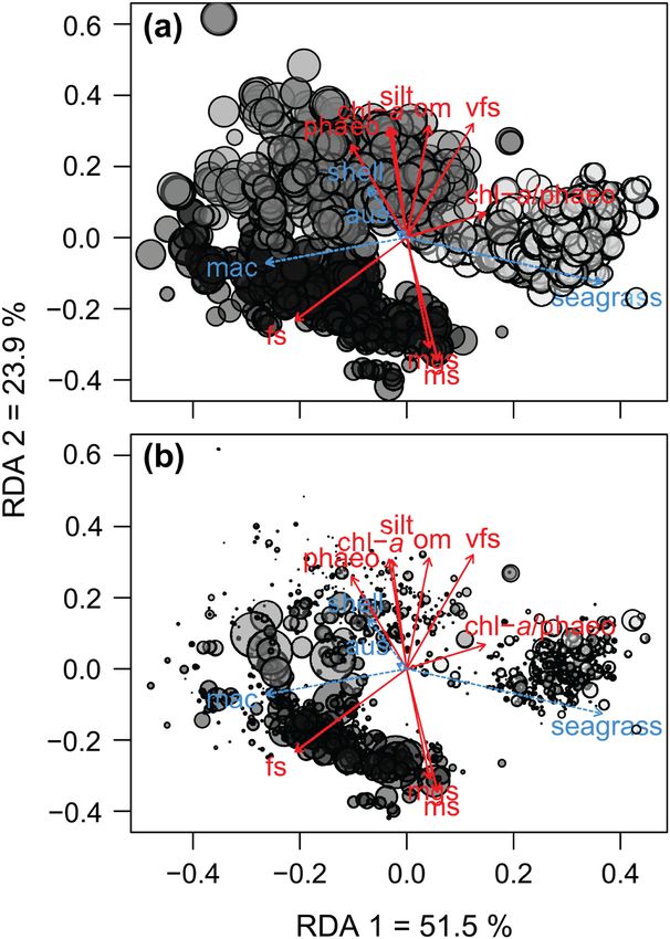
Figure 3. Venn diagrams of the variance partitioning based on environmental variation, and spatially structured abiotic and
dbRDA ordinations of the βSor (a), βSim (b) and βNes (c) at the biotic effects were the main contributors of β-diversity (βSor)
regional scale. Variance explained by the different explanatory com- among seascapes. The β-diversity differences among seascapes
ponents are shown in different colours: environmental variables in were mainly explained by species turnover (βSim), whereas
red, ecosystems engineers in green, large-scale among seascapes spa- richness differences (βNes) among sites were less important.
tial constraints in blue, and within seascapes spatial variation in The abundance of the bivalve M. liliana had a positive effect
grey. Values < 0 not shown.
on turnover, as observed by the dbRDA. This indicates that
the spatial structure of these bivalves can modify the environ-
Taxa replacement (βSim) was the component that most ment, indirectly structuring local communities with distinct
contributed to β-diversity at the regional scale with high composition from the background seascape.
replacement occurring within the Manukau (indicated by the More importantly, the various determinants of β-diversity
larger medium grey bubbles in Fig. 2a) at sites characterized did not simply operate at specific spatial scales. Therefore our
by higher percentages of shell-hash cover, fine sediments and initial expectations that 1) turnover (βSim) is influenced by
higher organic matter, chlorophyll-a and phytodetritus con- environmental drivers; 2) variations in the distribution of eco-
centrations (Fig. 2a). Lower replacement was observed in the system engineers contribute to β-diversity; and 3) large-scale
5Kaipara Manukau Tauranga
Env. Eng. Env. Eng. Env. Eng.
0.12 0.03 0.03 0.13 0.02 0.06 0.05 0.01 0.03
Beta-Sor
0.04 0.02 0.02
0.03 0.01 0.03 0.02 0.01
0.04 0.02 0.06
Space Space Space
Residuals = 0.70 Residuals = 0.72 Residuals = 0.80
Env. Eng. Env. Eng. Env. Eng.
0.15 0.04 0.03 0.15 0.03 0.08 0.05 0.00 0.03
Beta-Sim
0.06 0.02 0.03
0.04 0.01 0.03 0.02 0.01
0.04 0.02 0.08
Space Space Space
Residuals = 0.64 Residuals = 0.67 Residuals = 0.78
Env. Eng. Env. Eng. Env. Eng.
0.04 0.05 0.03
Beta-Nes
0.00
0.05 0.02 0.00
0.05
Space Space Space
Residuals = 0.95 Residuals = 0.93 Residuals = 0.88
Figure 4. Venn diagrams of the variance partitioning based on dbRDA ordinations of the βSor, βSim and βNes of single seascapes (Kaipara,
Manukau and Tauranga). Variance explained by the different explanatory components are shown in different colours: environmental vari-
ables in red, ecosystems engineers in green, large-scale among seascapes spatial constraints in blue, and within seascapes spatial variation in
grey. Values < 0 not shown.
spatial variation is more important to β-diversity than small- spatial constraints (neutral processes) and biotic interactions
scale variability, could be accepted. Importantly, the specific must be considered to fully understand the mechanisms of
role of each component cannot be disentangled from the oth- community assembly.
ers. Community structure within heterogeneous seascapes is The current view on metacommunity dynamics states
dependent on direct and indirect effects that operate over that both space and environment act together, and the
multiple spatiotemporal scales. Environmental variation has interdependency between these processes shape commu-
a key role in this dynamic, however our results stress that nities (Brown et al. 2017). Spatially structured abiotic
6gradients were important drivers of species turnover, suggest- and contribute to habitat heterogeneity (Hewitt et al. 2005).
ing that spatial autocorrelation affect seafloor biodiversity. This has important implications for habitat complexity in a
Environmental heterogeneity and community connectivity changing world (Hewitt et al. 2005, Blowes et al. 2019). For
are coupled and influence communities over multiples scales instance, regional and local decreases in population abun-
(Thrush et al. 2005, Kraan et al. 2015, Menegotto et al. dances of these habitat-forming species may boost biotic
2019). In our study, most of the β-diversity was captured by homogenization at the seafloor (Boyé et al. 2019). Moreover,
large-scale variability (among seascapes) whereas small-scale differences between range distribution and abundance of
variability (within-seascapes) only explained a small portion engineer species may have implications for community
of the variance in species composition. In addition, west coast resilience to disturbances and for biodiversity management
seascapes (Kaipara and Manukau) showed more similarity (Greenfield et al. 2016, Gladstone-Gallagher et al. 2019).
in community composition compared to Tauranga, which Macomona liliana is the most widespread species on Kaipara
is located in the east coast. This pattern could be related to and Manukau seascapes, whereas Austrovenus stutchburyi is
differences in geomorphology and in the regime of waves the most abundant at Manukau (Kraan et al. 2015). Hence,
and currents among coasts, but also to limited connectivity biotic engineers that are widespread across the seascape can
among the ecoregions (Ross et al. 2009). Therefore, neutral be more resilient to small-extent disturbances, while species
processes such as dispersal limitation and habitat connectiv- that occurred in smaller patches but in higher densities can
ity are important drivers of seafloor β-diversity (Thrush et al. be more sensitive.
2008). Hence, species life-history and dispersion potential, Sites in Tauranga on the contrary were characterized by
as well as disturbance–diversity relationships and prior- higher percentages of seagrass cover and lower abundances
ity effects, might be important for taxa turnover in marine of bivalves. The benthic community was also more homo-
ecosystems. geneous, showing a lower β-diversity at site scale than the
Environmental filtering is one of the most debated con- other two locations. This might suggest that seagrass mead-
cepts in modern ecology (Kraft et al. 2011, 2015, Thakur ows could provide a distinct habitat in the seascape, whereas
and Wright 2017), since it can determine the prevailing bivalve engineers tends to promote small-scale heterogeneity
mechanisms that drive community assembly, i.e. niche or in the sand habitat due to their bioturbation (Boström et al.
neutral processes (Leibold et al. 2004, Rosindell et al. 2011, 2010, Boyé et al. 2017, Kraan et al. 2020b). Moreover, sea-
Brown et al. 2017). We showed that in marine soft-bottoms, grass meadows might limit dispersion of infaunal species
environmental heterogeneity is a key driver of β-diversity, by reducing hydrodynamics and bedload transport, and
although, strongly interconnected with biotic engineering. their physical structure restricts bulldozing species, which
Therefore, the mechanisms influencing species turnover are may result in a lower species turnover within the seagrass
controlled by direct and indirect relationships of founda- habitat (Boström et al. 2010, Henseler et al. 2019). Seagrass
tion species with environmental gradients (Boyé et al. 2019, meadows provide substrate for both infauna and epifau-
Kraan et al. 2020b) and the resulting assembly pattern is taxa nal invertebrates (Boyé et al. 2017, Henseler et al. 2019).
dependent (Boyé et al. 2017, Henseler et al. 2019). Hence, These two components of benthic fauna can display distinct
communities inhabiting heterogeneous landscapes are shaped patterns of spatial variation, with epifauna in general
by multiple factors, including natural and human-driven showing lower β-diversity and high dominance of grazers
disturbances, trophic interactions, deterministic niche fac- than infauna, which suggest strong habitat filtering (Boyé
tors and stochasticity (Kraft et al. 2011, Mori et al. 2018, et al. 2017).
Limberger et al. 2019). For example, species dispersal is Natural and human-driven disturbances are constantly
strongly dependent on hydrodynamic regimes and species changing the seafloor, shaping communities over multiple
life-history traits (Lundquist et al. 2004, Rodil et al. 2017, spatial extents and frequencies (Gladstone-Gallagher et al.
2018) and can structure seafloor communities over mul- 2019, Solan et al. 2020). For instance, stingrays can forage
tiple scales (Lundquist et al. 2004, Moritz et al. 2013). The and disturb small patches of sediment at a high frequency,
effects of species competition are scale-dependent and are whereas trawling can disturb much larger extents of the sea-
more significant on the small-scale (Mod et al. 2020). On the floor at a different frequency. Biotic engineering operates
other hand, the effects of ecosystem engineering on commu- at multiple spatiotemporal scales, but is frequently over-
nity assembly are likely to propagate across different scales, looked in metacommunity dynamics (Wright et al. 2017).
which highlights the importance of seascape heterogeneity We advocate that the interdependence between space, envi-
for maintaining β-diversity and ecosystem functions at larger ronment and species interaction must be recognized, even
scales (Hewitt et al. 2008, Mod et al. 2020). in ecosystems where competition is not the main regulator
We found that biotic interactions significantly contrib- of biodiversity, such as the marine soft-bottom ecosystems,
uted to spatial turnover in species composition. Bivalves where food and space are not limiting factors. Ecosystem
can colonize large extents of the seafloor, changing sediment engineering and facilitation cascades can play a key role
biogeochemistry, food availability and habitat complexity in shaping β-diversity, recognizing their importance for
(Lohrer et al. 2013, Thrush et al. 2017). Furthermore, they biodiversity and ecosystem function is thus essential for
have a long legacy-effect in the environment, since calcium understanding the resilience of communities to multiple
carbonate shells last longer than the life span of the organism disturbances.
7Data availability statement Baselga, A. 2012. The relationship between species replacement,
dissimilarity derived from nestedness, and nestedness. – Global
Data available at Pangea Digital Repository (Kraan et al. 2019, Baselga, A. and Leprieur, F. 2015. Comparing methods to separate
2020a). components of beta diversity. – Methods Ecol. Evol. 6: 1069–1079.
Baselga, A. et al. 2018. betapart: partitioning beta diversity into
turnover and nestedness components. – R package ver. 1.5.1.
Acknowledgements – We are grateful to all NIWA staff that help .
with data gathering and sample processing, and to the Institute of Blowes, S. A. et al. 2019. The geography of biodiversity change in
Marine Science of University of Auckland for support this work. marine and terrestrial assemblages. – Science 366: 339–345.
Funding – MCB is supported by University of Auckland fellowship. Borcard, D. and Legendre, P. 2002. All-scale spatial analysis of
RGG was supported by the New Zealand Rutherford Foundation ecological data by means of principal coordinates of neighbour
Postdoctoral Fellowship and the Walter and Andrée de Nottbeck matrices. – Ecol. Model. 153: 51–68.
Foundation during the writing of this manuscript. Data collected Boström, C. et al. 2010. Invertebrate dispersal and habitat hetero-
under the Marsden fund of the Royal Society of New Zealand geneity: expression of biological traits in a seagrass landscape.
(NIW1102) to ST and a Marie-Curie International Outgoing – J. Exp. Mar. Biol. Ecol. 390: 106–117.
Fellowship (FP7-PEOPLE-2011-IOF, Nr. 298380) to CK. Boyé, A. et al. 2017. Constancy despite variability: local and
Conflict of interests – The authors declare that they have no known regional macrofaunal diversity in intertidal seagrass beds. – J.
competing financial interests or personal relationships that could Sea Res. 130: 107–122.
influence the work reported in this paper. Boyé, A. et al. 2019. Trait-based approach to monitoring marine
benthic data along 500 km of coastline. – Divers. Distrib. 25:
1879–1896.
Author contributions Brown, B. L. et al. 2017. Making sense of metacommunities: dis-
pelling the mythology of a metacommunity typology. – Oeco-
Marco C. Brustolin: Conceptualization (equal); Formal logia 183: 643–652.
analysis (lead); Investigation (equal); Methodology (equal); de Juan, S. et al. 2013. Counting on β-diversity to safeguard the
Software (lead); Validation (equal); Visualization (equal); resilience of estuaries. – PLoS One 8: e65575.
Writing – original draft (lead); Writing – review and editing Dirzo, R. et al. 2014. Defaunation in the Anthropocene. – Science.
(lead). Rebecca V. Gladstone-Gallagher: Conceptualization 345: 401–406.
(equal); Formal analysis (supporting); Funding acquisition Dray, S. et al. 2012. Community ecology in the age of multivariate
(supporting); Investigation (equal); Methodology (equal); multiscale spatial analysis. – Ecol. Monogr. 82: 257–275.
Validation (equal); Visualization (equal); Writing – original Eriksson, B. K. and Hillebrand, H. 2019. Rapid reorganization of
draft (supporting); Writing – review and editing (support- global biodiversity. – Science. 366: 308–309.
ing). Casper Kraan: Conceptualization (supporting); Data Gladstone-Gallagher, R. V. et al. 2019. Linking traits across eco-
logical scales determines functional resilience. – Trends Ecol.
curation (lead); Formal analysis (supporting); Investigation
Evol. 34: 1080–1091.
(equal); Methodology (equal); Supervision (supporting); Greenfield, B. L. et al. 2016. Mapping functional groups can pro-
Validation (equal); Visualization (equal); Writing – original vide insight into ecosystem functioning and potential resilience
draft (supporting); Writing – review and editing (support- of intertidal sandflats. – Mar. Ecol. Prog. Ser. 548: 1–10.
ing). Judi Hewitt: Conceptualization (supporting); Data Heino, J. 2013. Does dispersal ability affect the relative importance
curation (supporting); Formal analysis (supporting); Funding of environmental control and spatial structuring of littoral mac-
acquisition (supporting); Investigation (equal); Methodology roinvertebrate communities? – Oecologia 171: 971–980.
(equal); Project administration (equal); Resources (sup- Heino, J. et al. 2015. Metacommunity organisation, spatial extent
porting); Software (supporting); Supervision (supporting); and dispersal in aquatic systems: patterns, processes and pros-
Validation (equal); Visualization (equal); Writing – original pects. – Freshwater Biol. 60: 845–869.
draft (supporting); Writing – review and editing (support- Henseler, C. et al. 2019. Coastal habitats and their importance for
the diversity of benthic communities: a species- and trait-based
ing). Simon F. Thrush: Conceptualization (supporting); approach. – Estuar. Coast. Shelf Sci. 226: 106272.
Data curation (lead); Formal analysis (supporting); Funding Hewitt, J. E. et al. 2005. The importance of small-scale habitat struc-
acquisition (lead); Investigation (equal); Methodology ture for maintaining beta diversity. – Ecology 86: 1619–1626.
(equal); Project administration (lead); Resources (lead); Hewitt, J. E. et al. 2008. Habitat variation, species diversity and
Software (supporting); Supervision (lead); Validation (equal); ecological functioning in a marine system. – J. Exp. Mar. Biol.
Visualization (equal); Writing – original draft (supporting); Ecol. 366: 116–122.
Writing – review and editing (supporting). Hoegh-Guldberg, O. and Bruno, J. F. 2010. The impact of climate
change on the world’s marine ecosystems. – Science 328:
1523–1528.
References Ingram, T. and Shurin, J. B. 2009. Trait-based assembly and phy-
logenetic structure in northeast Pacific rockfish assemblages. –
Aller, R. C. and Cochran, J. K. 2019. The critical role of bioturba- Ecology 90: 2444–2453.
tion for particle dynamics, priming potential and organic C Kraan, C. et al. 2015. Cross-scale variation in biodiversity-environ-
remineralization in marine sediments: local and basin scales. – ment links illustrated by coastal sandflat communities. – PLoS
Front. Earth Sci. 7: 1–14. One 10: 1–12.
8Kraan, C. et al. 2019. Multi-scale data on intertidal macrobenthic Mori, A. S. et al. 2018. β-Diversity, community assembly and eco-
biodiversity and environmental features in Kaipara, Tauranga system functioning. – Trends Ecol. Evol. 33: 549–564.
and Manukau Harbours, New Zealand. – PANGAEA, . ronmental filtering and spatial structure on metacommunity
Kraan, C. et al. 2020a. Multi-scale data on intertidal macrobenthic dynamics. – Oikos 122: 1401–1410.
biodiversity and environmental features in three New Zealand Mouchet, M. A. et al. 2013. Invariant scaling relationship between
harbours. – Earth Syst. Sci. Data 12: 293–297. functional dissimilarity and co-occurrence in fish assemblages
Kraan, C. et al. 2020b. Co-occurrence patterns and the large-scale of the Patos Lagoon estuary (Brazil): environmental filtering
spatial structure of benthic communities in seagrass meadows consistently overshadows competitive exclusion. – Oikos 122:
and bare sand. – BMC Ecol. 20: 37. 247–257.
Kraft, N. J. B. et al. 2011. Disentangling the drivers of diversity Oksanen, J. et al. 2019. vegan: community ecology package. – R pack-
along latitudinal and elevational gradients. – Science 333: age ver. 2.5-5. .
1755–1758. Peres-Neto, P. R. et al. 2006. Variation partitioning of species data
Kraft, N. J. B. et al. 2015. Community assembly, coexistence and matrices: estimation and comparison of fractions. – Ecology 87:
the environmental filtering metaphor. – Funct. Ecol. 29: 2614–2625.
592–599. Rodil, I. F. et al. 2017. The role of dispersal mode and habitat
Legendre, P. 2008. Studying beta diversity: ecological variation par- specialization for metacommunity structure of shallow beach
titioning by multiple regression and canonical analysis. – J. invertebrates. – PLoS One 12: e0172160.
Plant Ecol. 1: 3–8. Rodil, I. F. et al. 2018. The importance of environmental and spatial
Legendre, P. 2014. Interpreting the replacement and richness dif- factors in the metacommunity dynamics of exposed sandy beach
ference components of beta diversity. – Global Ecol. Biogeogr. benthic invertebrates. – Estuar. Coasts 41: 206–217.
23: 1324–1334. Rosindell, J. et al. 2011. The unified neutral theory of biodiversity
Legendre, P. and Anderson, M. J. 1999. Distance-based redundancy and biogeography at age ten. – Trends Ecol. Evol. 26: 340–348.
analysis: testing multispecies responses in multifactorial eco- Ross, P. M. et al. 2009. Phylogeography of New Zealand’s coastal
logical experiments. – Ecol. Monogr. 69: 1–24. benthos. – N. Z. J. Mar. Freshwater Res. 43: 1009–1027.
Legendre, P. and De Cáceres, M. 2013. Beta diversity as the vari- Ruhí, A. et al. 2017. Interpreting beta-diversity components over
ance of community data: dissimilarity coefficients and parti- time to conserve metacommunities in highly dynamic ecosys-
tioning. – Ecol. Lett. 16: 951–963. tems. – Conserv. Biol. 31: 1459–1468.
Legendre, P. and Gallagher, E. D. 2001. Ecologically meaningful Sandwell, D. R. et al. 2009. Density dependent effects of an infau-
transformations for ordination of species data. – Oecologia 129: nal suspension-feeding bivalve Austrovenus stutchburyi on sand-
271–280. flat nutrient fluxes and microphytobenthic productivity. – J.
Leibold, M. A. et al. 2004. The metacommunity concept: a frame- Exp. Mar. Biol. Ecol. 373: 16–25.
work for multi-scale community ecology. – Ecol. Lett. 7: Solan, M. et al. 2020. Benthic-based contributions to climate
601–613. change mitigation and adaptation. – Phil. Trans. R. Soc. B 375:
Li, F. et al. 2020. Local contribution to beta diversity is negatively 20190107.
linked with community-wide dispersal capacity in stream inver- Thakur, M. P. and Wright, A. J. 2017. Environmental filtering,
tebrate communities. – Ecol. Indic. 108: 105715. niche construction and trait variability: the missing discussion.
Limberger, R. et al. 2019. Spatial insurance in multi-trophic meta- – Trends Ecol. Evol. 32: 884–886.
communities. – Ecol. Lett. 22: 1828–1837. Thrush, S. et al. 2005. Multi-scale analysis of species–environment
Lohrer, A. M. et al. 2013. Biogenic habitat transitions influence relationships. – Mar. Ecol. Prog. Ser. 302: 13–26.
facilitation in a marine soft-sediment ecosystem. – Ecology 94: Thrush, S. F. et al. 2008. The effects of habitat loss, fragmentation
136–145. and community homogenization on resilience in estuaries.
Lundquist, C. J. et al. 2004. Limited transport and recolonization – Ecol. Appl. 18: 12–21.
potential in shallow tidal estuaries. – Limnol. Oceanogr. 49: Thrush, S. F. et al. 2017. Changes in the location of biodiversity–
386–395. ecosystem function hot spots across the seafloor landscape with
Mason, N. W. H. et al. 2011. Niche overlap reveals the effects of increasing sediment nutrient loading. – Proc. R. Soc. B 284:
competition, disturbance and contrasting assembly processes in 20162861.
experimental grassland communities. – J. Ecol. 99: 788–796. Turner, S. et al. 1997. Bedload and water-column transport and colo-
Maynard, D. S. et al. 2020. Predicting coexistence in experimental nization processes by post-settlement benthic macrofauna: does
ecological communities. – Nat. Ecol. Evol. 4: 91–100. infaunal density matter? – J. Exp. Mar. Biol. Ecol. 216: 51–75.
McGill, B. J. et al. 2015. Fifteen forms of biodiversity trend in the Ulrich, W. et al. 2018. Functional traits and environmental char-
anthropocene. – Trends Ecol. Evol. 30: 104–113. acteristics drive the degree of competitive intransitivity in Euro-
Menegotto, A. et al. 2019. The scale-dependent effect of environ- pean saltmarsh plant communities. – J. Ecol. 106: 865–876.
mental filters on species turnover and nestedness in an estuarine van Buuren, S. and Groothuis-Oudshoorn, K. 2011. mice: multi-
benthic community. – Ecology 100: e02721. variate imputation by chained equations in R. – J. Stat. Softw.
Mod, H. K. et al. 2020. Scale dependence of ecological assembly 45: 1–67.
rules: insights from empirical datasets and joint species distribu- Wright, A. J. et al. 2017. The overlooked role of facilitation in bio-
tion modelling. – J. Ecol. 108: 1967–1977. diversity experiments. – Trends Ecol. Evol. 32: 383–390.
9You can also read