ECONtribute Discussion Paper - Are Economists' Preferences Psychologists' Personality Traits? A Structural Approach
←
→
Page content transcription
If your browser does not render page correctly, please read the page content below
ECONtribute
   Discussion Paper

Are Economists’ Preferences Psychologists’ Personality
           Traits? A Structural Approach

                                         Tomáš Jagelka

                                             July 2020
                        ECONtribute Discussion Paper No. 014

    Funding by the Deutsche Forschungsgemeinschaft (DFG, German Research Foundation) under Germany´s
                   Excellence Strategy – EXC 2126/1– 390838866 is gratefully acknowledged.

                                         Cluster of Excellence

                                                                                        www.econtribute.de
W ORKING PAPER

                Are Economists’ Preferences
         Psychologists’ Personality Traits?
              A Structural Approach

                                                 Author:
                                        Tomáš J AGELKA‡

                                              May 26, 2020

   I would like to give special thanks to Christian Belzil, James Heckman, Douglas Staiger, John Rust and four
anonymous referees for their detailed feedback and to Frederik Bennhoff, Raicho Bojilov, Alexandre Cazenave-
Lacroutz, Femke Cnossen, Thomas Dohmen, Armin Falk, Erzo Luttmer, Julie Pernaudet, Andrew Samwick,
Sieuwerd Gaastra and Jonathan Zinman for their helpful comments. I also thank participants at seminars at
Dartmouth College, École Polytechnique - CREST, Georgetown University, the University of Chicago, the Uni-
versity of Bonn, CERGE-EI, at the RES annual conference, the RES PhD meetings, the RES junior symposium,
and at the annual conference of the Slovak Economic Association for their feedback. I gratefully acknowledge the
receipt of the Student Travel Grant for the IAAE 2019 conference and of the prize for the “Best paper presented
by a graduate student” at the conference. This research is funded by the Deutsche Forschungsgemeinschaft (DFG,
German Research Foundation) under Germany´s Excellence Strategy – EXC 2126/1– 390838866.
  ‡
    ECONtribute Cluster of Excellence, IZA, Institute for Applied Microeconomics at the University of Bonn, and
CEHD at the University of Chicago. Email: tjagelka@uni-bonn.de.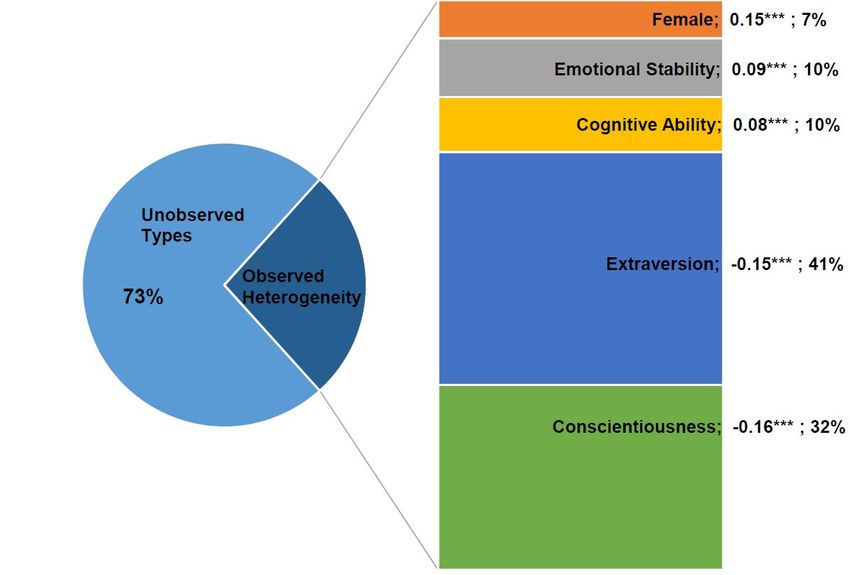
Abstract
This paper proposes a method for empirically mapping psychological personality traits to eco-
nomic preferences. Careful modelling of random components of decision making is crucial
to establishing the long supposed but empirically elusive link between economic and psycho-
logical systems for understanding differences in individuals’ behavior. I use factor analysis
to extract information on individuals’ cognitive ability and personality and embed it within
a Random Preference Model to estimate distributions of risk and time preferences, of their
individual-level stability, and of people’s propensity to make mistakes. I explain up to 50% of
the variation in both average risk and time preferences and in individuals’ capacity to make
consistent rational choices using four factors related to cognitive ability and three of the Big
Five personality traits. True differences in desired outcomes are related to differences in per-
sonality whereas actual mistakes in decisions are related to cognitive skill.
1 Introduction
There is extensive evidence that economic preferences, cognitive ability, and personality pre-
dict a wide range of economic outcomes (see Heckman, Jagelka, and Kautz, 2019 for a recent
summary of the literature). However, the question of whether they work through one another
or side by side had not been conclusively answered. It is important to do so in order to deter-
mine the dimension of attributes which constitute human capital and explain differences in life
outcomes.1 I demonstrate that careful modelling of random errors allows one to establish the
long supposed but empirically elusive link (see Almlund et al., 2011 and Becker et al., 2012)
between economic and psychological frameworks for understanding differences in individuals’
behaviors.
I estimate a structural model of decision making under uncertainty and delay using data from a
unique field experiment in which each participant made over 100 choices on incentivized tasks
designed to elicit risk and time preferences. There are 5 estimated structural parameters of
interest: the coefficient of risk aversion and the discount rate which measure true (or average)
risk and time preferences respectively; two parameters which describe the degree of instability
of an individual’s risk and time preferences respectively; and a “mistake” parameter which
allows an individual to choose his less preferred option some percentage of the time. I use
the extensive associated survey data to map both true economic preferences and the stochastic
components of decision-making onto cognitive ability and factors related to three of the Big
Five personality traits.
Both true risk and time preferences and their associated stochastic components map robustly
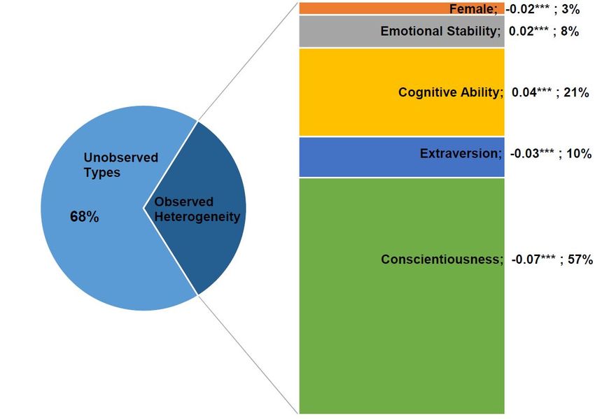
onto cognitive ability and personality. Overall, the conscientiousness trait exhibits the strongest
links. It explains a third of the cross-sectional variation in discount rates, 9% of the variation
in risk aversion, and 23% of the variation in their individual-level stability. Furthermore, ex-
traversion is strongly related to risk aversion and discount rates while high cognitive ability
reduces an individual’s propensity to make mistakes. The latter confirms Andersson et al.’s
(2016) suspicion that the failure to properly account for the presence of random errors and of
their link to observables likely resulted in biased estimates of both risk aversion and of its
relationship with characteristics such as cognitive ability in previous research.
My results show that heterogeneity in preferences explains a majority of the variation in ob-
served choices between risky lotteries and between payments occurring at different points in
time. Indeed, the five estimated structural parameters alone have explanatory power which is
an order of magnitude larger than that of nearly two dozen demographic and socio-economic
1
There is an increasing recognition in educational systems and beyond that characteristics other than cognitive
ability are important. However, there is currently a lack of consensus on which ones truly matter and how to
measure them.
1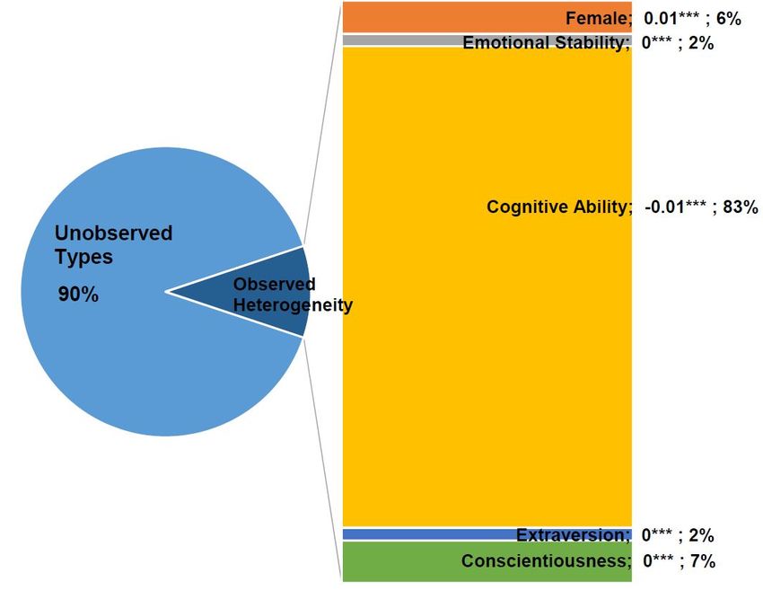
variables. While risk and time preferences account for a vast majority of the explained varia-
tion in the overall number of risky or intertemporal choices, parameters related to randomness
in decision making also have a non-negligible influence and predict inconsistencies in individ-
ual behavior. I thus call them consistency parameters.

My structural model has two main parts: a factor model used to derive latent cognitive ability
and personality traits from multiple noisy observed indicators; and a model of decision-making
under uncertainty and delay based on the assumption that decisions are driven by expected
utility maximizing behavior which itself depends on an individual’s risk and time preferences
but is subject to random errors. I allow preferences to depend both on observed heterogeneity
and on unobserved factors related to cognitive ability and personality. In addition, I allow the
structural parameters of the model to depend on “true” unobserved heterogeneity (unrelated
to any observed characteristics or measures) in the form of unobserved types.

I estimate the model empirically through simulated maximum likelihood using data from “The
Millenium Foundation Field Experiment on Education Financing” based on a representative
sample of 1,224 Canadian high school seniors. An individual’s likelihood contribution is the
probability of jointly observing his choices on A) 55 incentivized tasks designed to elicit risk
preferences, B) 48 incentivized tasks designed to elicit time preferences, and C) his answers
to 38 questions designed to measure cognitive ability and personality, all given his observed
characteristics, the four unobserved latent factors2 , and five unobserved types.3

My approach generalizes to settings in which one wishes to relate parameters of economic
models to observables with multiple available noisy measures. It incorporates a flexible error
structure which accounts for errors in both decision making and in measurement, and thus
allows to separate signal from noise in observed choices.

The rest of the paper is organized as follows: Section 2 situates my contribution within the
broader economic and psychological literature, Section 3 describes the data, Section 4 presents
the theoretical underpinnings of the structural model, Section 5 details the empirical method-
ology, Section 6 presents the empirical results, Section 7 provides a general discussion of the
broader implications of the findings presented in this article, and Section 8 concludes.
  2
      The factors of interest are: an individual’s cognitive skills and his personality traits. The latter consist of
factors related to emotional stability, extraversion, and conscientiousness: stable personality traits identified by
psychologists as particularly important predictors of behavior and part of the Big Five personality traits. These
factors have been chosen to capture both “soft” and “hard” skills given measures available in the data.
   3
     The joint estimation of all three components of the structural model allows for an optimal use of the informa-
tion in the dataset. Furthermore, failure to estimate risk and time preferences jointly has been shown to lead to
unrealistically high estimates of the discount rate (see Andersen et al., 2008 and 2014; Cohen et al., 2016).

                                                          2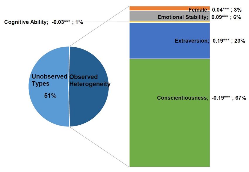
2         Background

2.a         Relating Preferences and Personality

This paper builds on previous research in both economics and psychology. Walter Mischel’s
work on the “Marshmallow Test” brought attention to the importance of enduring traits in life
outcomes. He found that children who were able to resist temptation to immediately eat one
marshmallow and instead wait 15 minutes to get several, had better SAT scores, educational
attainment, etc. later in life. Their choice to defer immediate gratification thus seemed to
reflect some characteristic - preference or skill - which is valuable in other contexts. It would
be explained by a low discount factor in neoclassical economic models and associated with
the conscientiousness personality trait in the psychological literature. Similar intuitive corre-
spondences can be drawn between diverse economic preferences4 and personality traits5 . In
their 2017 review of the literature, Golsteyn and and Shildberg-Horisch note that “research on
preferences and personality traits is a blossoming field in economic and psychological science.
Economic preferences and personality traits are related concepts in the sense that both are
characteristics of an individual that have been shown to predict individual decision making
and life outcomes across a wide variety of domains.”

Attempts to relate economic preferences and psychological traits can be understood as part of a
broader effort to determine the dimensionality of attributes - skills, preferences, or behavioral
biases - required to characterize essential human differences. One strand of the literature at-
tempts to create “an empirical basis for more comprehensive theories of decision-making” by
correlating various behavioral measures and sorting them into clusters (e.g. Chapman et al.,
2018 and Dean and Ortoleva, 2019). A second strand concerns itself with summarizing the var-
ious documented behavioral tendencies in a simplified measure like a sufficient statistic (e.g.
Chetty, 2015) or a sparsity model (e.g. Gabaix, 2014). Stango and Zinman (2019) empirically
test such “B-counts” constructed from various behavioral biases relevant in consumer finance
and find that they are correlated with cognitive ability and predictive of financial outcomes.
    4
        Risk and time preference are the most basic economic preferences. Along with differences in constraints,
they explain heterogeneity in behavior in neoclassical economic models. They are standardly embodied by the
coefficient of risk aversion and by the discount factor respectively. More recent economic theory also incorporates
social preferences and behavioral biases.
   5
     Roberts (2009) characterizes personality traits as “the relatively enduring patterns of thoughts, feelings, and
behaviors that reflect the tendency to respond in certain ways under certain circumstances.” While various classi-
fications exist, the Big Five is the most prominent. It consists of: Extraversion associated with excitement-seeking
and active, sociable behavior; Conscientiousness associated with ambition, self-discipline, and the ability to delay
gratification; Emotional stability associated with confidence, high self-esteem, and consistency in emotional reac-
tions; Agreeableness associated with warmth, trust, and generosity; and Openness to experience associated with
imagination and creativity.

                                                         3
My contribution is to show that up to 50% of the heterogeneity in both the true (or average)
risk and time preferences, in their individual-level stability, and in people’s propensity to make
mistakes can be explained by cognitive ability and factors related to three of the Big Five per-
sonality traits: extraversion, conscientiousness, and emotional stability.6 Defined as stable,
person-specific determinants of behavior, they are the natural counterparts of economic pref-
erences in the psychology literature. Indeed, they have been shown to predict many of the
same real-world outcomes (see Heckman, Jagelka, and Kautz, 2019). However, despite this
“intuitive mapping of preferences to traits, the empirical evidence supporting such mappings
is weak. The few studies investigating empirical links typically report only simple regressions
or correlations without discussing any underlying model.” (Almlund et al., 2011)7
This paper is the first attempt to establish such a mapping in a full structural framework of
decision-making under uncertainty and delay.8 The amount of explained cross-sectional vari-
ation is large compared to previous research (see for example Becker et al, 2012). My results
suggest that preferences and personality do not simply function side by side as previously
claimed but that they are strongly related. I believe that I find a stronger relationship than
previous studies because I estimate each trait from multiple noisy indicators using a factor
model embedded in a full structural model of decision-making. This makes optimal use of
available information and should address attenuation bias resulting from measurement er-
ror (see for example Carneiro, Hansen, and Heckman, 2003; Cunha and Heckman, 2009; and
Cunha, Heckman, and Schennach, 2010) as well as decision error bias (see Andersson et al.,
2016). Because preferences and traits as well as the quality of decision making have been
shown to predict outcomes and to be highly heritable, this finding also has ramifications for
understanding inequality and the mechanisms underlying the inter-generational transmission
of socio-economic status.9
6
While this dataset did not measure the Big Five personality traits using a questionnaire specifically developed
for this purpose, the available survey questions listed in Section 10.b of the Appendix provide reasonable proxies
for the first three traits. This assumption is supported by the fact that I obtain similar results - low correlations
between preferences and personality - as those reported in previous research (e.g. Becker et al., 2012) when
relying on reduced form measures used in that research i.e. on the average numbers of safe or patient choices to
proxy for risk and time preferences respectively and on measures of cognitive ability and personality constructed
as a simple sum of the constituent indicators.
7
The question is as valid now as it was nine years ago. In a 2018 Journal of Economic Perspectives symposium
on “Risk in Economics and Psychology”, Mata et al., 2018 mention the need “to make conceptual progress by
addressing the psychological primitives or traits underlying individual differences in the appetite for risk.”
8
In a contemporaneous project, Andersson et al. (2018) employ a similar theoretical model. As the focus of their
study is on de-biasing inference based on lottery choice tasks, their work is limited to the study of risk preferences.
The correlations between risk aversion and personality which they obtain point to the same general direction as
my results. My framework and rich data allow me to dig deeper and establish a comprehensive mapping showing
the percentage of cross-sectional variation in risk preference (and in time preference as well as in parameters
governing decision instability) explained by cognitive ability and three factors related to personality.
9
Heritability estimates are about 50% for cognitive skills and personality (see for example Bouchard and
Loehlin, 2001; and Bergen, Gardner, and Kendler, 2007). Evidence is more mixed regarding the heritability
4If preferences influence outcomes also through one another, this has implications for specify-
ing reduced form and structural economic models and for accurately interpreting their results.
On the one hand, I corroborate Von Gaudecker, Van Soest, and Wengstrom’s (2011) claim that
preferences contain much more useful information than that which could be captured by socio-
demographics alone and that they should therefore be used to complement the standard set of
controls used in empirical research aimed at explaining heterogeneity in economic outcomes. I
find that preferences dominate demographic and socio-economic variables when it comes to ex-
plaining the variation in observed choices under risk and delay. On the other hand, I show that
when this is not possible, omitted variable bias could potentially still be alleviated by adding
controls for ability and personality as those are heavily correlated with preferences when prop-
erly measured. Using only the coefficients from my structural model, information on observed
heterogeneity, and my estimates of the prevalence of unobserved types, I am able to simulate
as rich a distribution of preferences and of the random components of decision-making as can
be obtained from estimates based on the full set of observed individual choices. For compar-
ison purposes, using observed and unobserved heterogeneity, Von Gaudecker, Van Soest, and
Wengstrom (2011) can cover only about one third of the distribution of risk preferences which
they obtain using information on individual choices on incentivized tasks designed to elicit risk
preferences.
Nevertheless, I find that a large part of the cross-sectional variation is attributable to unob-
served heterogeneity embodied by unobserved types. Establishing a more complete mapping
between economic and psychological measures of human differences will require further re-
search relying on enhanced datasets with an expanded array of economic preferences and the
full Big Five.
2.b Separating Signal From Noise in Observed Measures
When elicited within laboratory experiments, risk and time preferences are difficult to esti-
mate without introducing a stochastic element capturing a form of seemingly erratic behavior.
For instance, take a classical Multiple Price List (MPL) approach popularized by Holt and
Laury (2002) in which individuals face a sequence of binary choices between lotteries. Typi-
cally, the attractiveness of the riskier alternative increases as one proceeds down a set of tasks
of an MPL. Certain individuals who at some point switch to the riskier option revert back to
the safer one in subsequent choices even if those offer an even more attractive riskier alterna-
of preferences although recent research has shown that they may be as heritable as cognitive and non-cognitive
traits (see for example Beauchamp, Cesarini, and Johannesson, 2017). Little is known regarding the heritability
of decision-making quality. My results documenting a strong link between preferences, random components of
decision-making, cognitive skill, and personality combined with extensive psychological research on the heritabil-
ity of personality suggest that all of the above may be heritable to a large degree.
5tive. Furthermore, when faced with multiple sets of questions designed to elicit risk (or time)
preferences, individuals rarely make choices consistent with having one precise parameter for
risk (or delay) aversion. For this reason, individual behavior can be naturally characterized
by structural preference parameters such as the coefficient of relative risk aversion or the
discount factor but also by parameters representing the propensity to deviate from their true
(or average) preferences. Let us call the latter consistency parameters.
Accordingly, economists developed stochastic choice models that introduce a noise element into
individual decisions. The Random Utility Model (RUM) includes the often used Fechner and
Luce error specifications and has been largely favoured by experimentalists (e.g. Hey and
Orme, 1994; Holt and Laury, 2002; Andersen et al., 2008). While there are multiple varia-
tions of the framework (see Becker, DeGroot, and Marschak, 1963), it can be modeled as an
error term appended to the utility that a decision maker derives from selecting a particular
alternative, thus making choices probabilistic. Under RUM, noise is standardly assumed to be
independent of the structural expected utility component driving decisions. Choice probabil-
ities derived using the RUM thus exhibit non-monotonicities which are at odds with a basic
theoretical definition of risk and time preferences, calling into question its continued use in
preference estimation. Recent papers by Wilcox (2011) and Aspesteguia and Ballester (2018)
have pointed out the benefits of using a different type of stochastic model in which the error
term directly impacts individual preference parameters. This type of error specification was
proposed by Loomes and Sugden (1995). While it can be considered a particular interpretation
of the broad random utility framework, for the sake of clarity of terminology, I will refer to it as
the Random Preference Model (RPM) following its authors. Bruner (2017) provides empirical
support for the use of monotone models in risk preference estimation by documenting a nega-
tive relationship between risk aversion and stochastic decision error as predicted by this class
of models (RUM has the opposite prediction).10 Aspesteguia and Ballester (2018) compared the
RUM to the RPM model with decision errors11 within a representative agent framework using
Danish data. Their estimates indicate that the degree of relative risk aversion obtained from a
RUM specification is lower than the estimate obtained using a RPM, especially for individuals
who are highly risk-averse. However, they do not investigate the distributions of preference
parameters using the RPM. Indeed, a structural estimation of the distributions of preference
(let alone consistency) parameters, has not yet been performed within this framework.
I contribute to this active area of research by estimating distributions of risk and time prefer-
ences using the Random Preference Model (RPM). I am the first to jointly estimate full popu-
10
The predicted general relationship between decision errors and risk aversion under RPM is actually more
complex. However, in choices in which both alternatives have the same expected return and differ only in its
variance (such as those used by Bruner, 2017, to detect mistakes), the predicted relationship is indeed negative.
11
Incorporating a “mistake” parameter within the RPM framework allows for “processing error” on the part
of the decision-maker. It relaxes the otherwise strong rationality requirements of the RPM which for example
excludes choosing dominated options.
6lation distributions of risk and time preference parameters and of their associated stochastic
components using the RPM framework. Even though my estimates are based on a popula-
tion which is largely homogeneous in terms of educational level and age, I find significant
dispersion in risk and time preferences, in their individual-level precision, and in the agents’
propensity to make random mistakes. This suggests that it may not be sufficient to use a
simple population average of risk and time preferences in the calibration of structural models
as has often been done before. Because preference parameters factor non-linearly into a wide
range of microeconomic and macroeconomic models, such a simplification is likely to have ram-
ifications for predicting agents’ responses to changes in economic conditions and for calculating
the welfare implications of new policy.
My approach offers a comprehensive treatment of random errors associated with both the
stability of preferences and with the propensity to make random mistakes. While the addition
of various types of stochastic components to models of decision-making is not new, my approach
is unique in that I introduce a total of three distinct consistency parameters and that I let each
of them be a function of both observed and unobserved heterogeneity.
I build on a rich literature concerned with separating out true preferences from stochastic
components affecting decision-making. Beauchamp, Cesarini, and Johannesson (2017) find
that simply accounting for measurement error improves the test-retest predictability of risk
preferences in repeated samples and provides tighter estimates of their relationship with per-
sonality traits. Bruner (2017) finds that errors decrease with risk aversion. He estimates
risk preferences from standard MPLs and error propensity from the number of choices of a
stochastically dominated option in separate choice tasks. In the absence of a structural model
he is not able to use the individual noise estimates to correct estimated risk aversion and thus
simply takes the average switching point from two MPL lists to reduce measurement error, a
commonly used but imprefect solution. Several recent papers (e.g. Stango and Zinman, 2019
and Chapman et al., 2018) refer to Gillen et al. (2019) to use multiple measures of a variable
as instruments for one another to reduce measurement error. While this approach is valid, it
is not as original as claimed.12 Moreover, it does not deal with decision error mentioned by
Andersson et al. (2016) who suggest that random mistakes, if not properly accounted for, may
bias preference estimates.13
Insofar as decision errors depend on observed and unobserved heterogeneity, they can also
lead to the detection of spurious correlations between estimated preferences and explanatory
variables (e.g. between risk aversion and cognitive ability). Andersson et al. (2018) empir-
12
The estimation system follows directly from Hansen (1982) or Sargan (1958).
13
E.g. if an average person tends to choose the risky option on 8 out of 10 MPL tasks, random mistakes will
more likely turn his choice to safe than to risky, leading to an overestimation of risk aversion. This will be true
also in repeated measurements making errors in the risky behavior variable correlated between the measure and
its instrument, thus invalidating the instrument.
7ically document the existence of decision error bias using two MPLs calibrated such that a
risk neutral decision maker switches at a different point in each MPL.14 They find that only
a combination of their “balanced” design and of the use of an RPM with heterogeneous noise
eliminates the spurious negative correlation between risk aversion and cognitive ability in-
duced by a standard MPL (such as those studied in this paper).15 In contrast, my results
suggest that given enough observed lottery choices per individual, a more sophisticated RPM
framework which I develop in this paper and which includes unobserved heterogeneity and a
factor model, is in itself sufficient to eliminate the spurious negative correlation between risk
aversion and cognitive ability.
Von Gaudecker, Van Soest, and Wengstrom (2011) come perhaps the closest to my treatment of
random errors. They include both a parameter representing the stability of individuals’ choices
under risk and a “trembling hand” parameter which embodies completely random decision-
making some percentage of the time. However, while they admit that it would be useful to let
both error types be individual-specific, they say that “in practice it appears to be difficult to
estimate heterogeneity in [them] separately (although both are identified, in theory)”. I can
do so, as I have a large number of incentivized choice tasks per individual, some designed to
elicit risk preferences and others time preferences. On the one hand, stability parameters – the
standard deviation of the coefficient of risk aversion and the standard deviation of the discount
rate – are identified from small inconsistencies in choices centered around an individual’s true
or average preference for risk and time respectively. On the other hand, the trembling hand
parameter related to an individual’s propensity to make mistakes is identified from situations
in which he chooses either strictly dominated options or makes choices far from his average
preferences. Accordingly inconsistent switching points across MPLs are best explained by the
estimated stability parameters whereas actual choice reversals within a given MPL (a much
stronger violation of choice consistency) are best explained by the estimated trembling hand
parameter.
I document a relationship between preference instability and conscientiousness, and between
the propensity to make mistakes and cognitive ability supporting the notion that these two
types of choice inconsistency are fundamentally separate. More conscientious individuals ex-
hibit more stable risk and time preferences while higher ability individuals make errors in
decisions less frequently.
14
Their logic behind such a “balanced design” is that in each MPL, the bias on estimated risk aversion due to the
existence of random mistakes (e.g. a person picks the riskier option when in fact the safe one is truly preferred)
should go in a different direction and thus balance out. In order for this to work in practice, one would need an
MPL design balanced at the individual level according to each individual’s true level of risk aversion.
15
This design is characterized by a relatively early switching point to the risky lottery. If lower cognitive ability
individuals make more mistakes, the spurious negative correlation between risk aversion and cognitive ability
emerges.
8The stability parameters allow individuals’ tastes to vary. Having estimates of the standard
deviation of the coefficient of risk aversion and of the discount rate lets me obtain distributions
of preferences complete with information on their individual-level precision. I take the view
that estimated preference instability does not necessarily point to irrational behavior. For
example, in my model, an individual would still be choosing his preferred alternative according
to expected utility maximization given the “instantaneous” draw of risk preference from his
distribution of the coefficient of risk aversion. Revealed preferences could be unstable due to
imperfect self-knowledge (for example, an individual may be uncertain whether he requires
a 8.1% or 8.2% rate of return when trading off between payments across time and thus he
may choose to randomize within this interval) or they could vary due to external factors such
as rising temperature in the room. Alternatively, these stability parameters can be viewed as
akin to measurement error describing the degree of precision to which I can measure a person’s
true (or average) preferences from his observed choices.16 While the economic interpretation
of my results may be different depending on whether one or the other hypothesis is true, both
reflect the fact that individuals exhibit various degrees of choice inconsistency even on simple
tasks performed in controlled laboratory environments which cannot be fully explained by
variation alone in task parameters.
The trembling hand parameter allows for individuals to make mistakes and actually pick their
less preferred alternative some percentage of the time. This can be due some individuals hav-
ing a level of cognitive ability which is either insufficient to correctly process the parameters
of the choice task at hand or which would require too much effort relative to the experimental
payoffs. This hypothesis is supported by my finding that heterogeneity in the trembling hand
parameter is best explained through variation in cognitive ability. In contrast, heterogeneity
in both true preferences and in preference instability (which leads to choosing the currently
preferred option although this may be inconsistent with the individual’s true underlying pref-
erence) is best explained by personality traits. A pattern emerges: Differences in desired out-
comes (which themselves may vary) are related to differences in personality whereas mistakes
in decisions which result in actually choosing the less preferred option are related to cognitive
skill.
The existence of heterogeneity in consistency parameters which characterize the stochastic
components of decision-making may have a large impact on economic outcomes. Since El-
Gamal and Grether’s finding that students from better colleges behave in a more bayesian
way, a body of evidence has accumulated showing a link between cognitive ability and vari-
ous types of behavioral biases and inconsistencies (e.g. Benjamin, Brown, and Shapiro, 2013;
16
Or, in the words of Loomes and Sugden (1995): “the stochastic element derives from the inherent variability
or imprecision of the individual’s preferences, whereby the individual does not always know exactly what he or
she prefers. Alternatively, it might be thought of as reflecting the individually small and collectively unsystematic
impact on preferences of many unobserved factors.”
9Choi et al., 2014; and Stango and Zinman, 2019). Choi et al. (2014) show that the quality of
decision-making measured as consistency of choices with the general axiom of revealed pref-
erence (GARP) has a casual impact on the variation in accumulated lifetime wealth. While
making mistakes can clearly be costly in many situations, the point is slightly more subtle
when it comes to preference instability. Individuals with less stable preferences may be penal-
ized in environments like the stock market which tend to reward stable, long-term decisions.
One could construct an index of decision-making consistency which would reflect an individ-
ual’s position on the joint distribution of the three consistency parameters (akin to Choi et al.’s,
2014 index based on the GARP). If cognitive ability and personality traits are assumed to func-
tion also as primitives of economic models through (or alongside) preferences, their combined
impact on outcomes such as accumulated wealth may be further magnified: for example take
a situation in which conscientiousness makes an individual do well financially both through
its direct impact on his career success and indirectly through a lower associated discount rate
which will induce him to make better savings and investment decisions.
3 Data
The data comes from “The Millenium Foundation Field Experiment on Education Financing”
which involved a representative sample of 1,224 Canadian citizes who were full time students
in their last year of high school. The students were between 16 and 18 years old at the time of
the experiment.
The experiment was conducted using pen and paper choice booklets as well as simple random
sampling devices like bingo balls and dice. Project cost considerations suggested that partici-
pants be drawn from locations with convenient travel connections from the SRDC Ottawa and
CIRANO Montreal offices. Manitoba, Saskatchewan, Ontario and Quebec were the selected
provinces. The implementation team was able to carry out work in urban and rural schools in
each of the four provinces.
The experiment contains 103 choice tasks designed to elicit risk and time preferences. Choices
were incentivized and students were paid for one randomly drawn decision at the end of the
session. The full experimental setup is included in Section 2 of the Online Appendix.
3.a Holt & Laury’s (H&L) Multiple Price List Design
Of the 55 tasks designed to measure risk aversion, the first 30 are of the Holt and Laury
(H&L) type introduced by Miller, Meyer, and Lanzetta (1969) and used in Holt and Laury
(2002). Choice payments and probabilities are presented using an inuitive pie chart repre-
10sentation popularized by Hey and Orme (1994). There are 3 groups of 10 questions. In each
group of questions, subjects are presented with an ordered array of binary lottery choices. In
each choice task they choose between lottery A (safer) and lottery B (riskier). In each subse-
quent row, the probability of the higher payoff in both lotteries increases in increments of 0.1.
While the expected value of both lotteries increases, the riskier option becomes relatively more
attractive. As in the first row of each set of questions the expected value of the safer lottery
A is greater than that of the riskier lottery B, all but risk-seeking individuals should choose
the safer option. Midway through the 10 questions, the expected value of the riskier lottery
B becomes greater than that of the safer lottery A. At this point, risk neutral subjects should
switch from the safer to the riskier option. In the remaining rows the relative attractiveness of
lottery B steadily increases until it becomes the dominant choice in the last row.17 By the last
row of each set of H&L questions, all individuals are expected to have switched to the riskier
option. Each person’s “switching point” should be indicative of his risk aversion. By design,
in the absence of a shock to either his preferences or utility, each individual should switch at
exactly the same point on the 3 sets of H&L questions.18
3.b Binswanger’s Ordered Lottery Selection (OLS) design
The remaining 25 tasks designed to measure risk aversion used in this study are a binarized
version of the ordered lottery selection (OLS) design developed by Binswanger (1980) and pop-
ularized by Eckel and Grossman (2002 and 2008). They consist of 5 groups of 5 questions.
Once again, in each group of questions, subjects are presented with an ordered array of bi-
nary lottery choices. In each choice task they choose between lottery A (safer) and lottery B
(riskier). This time, lottery A offers a certain amount in the first row and all other alternatives
increase in expected payoff but also in its variance. In each subsequent row the riskier option
becomes relatively less attractive. Individuals are thus expected to switch from the risky to the
safe option at some point (assuming that they initially picked the risky option). Once more,
the “switching point” should be indicative of each individual’s risk preferences. It should vary
among the 5 sets of OLS type questions for a given individual, unlike in the H&L design. How-
ever, a risk neutral individual should always at least weakly prefer the riskier alternative. In
the absence of stochastic shocks to utilities of preferences, the H&L tasks should allow for the
identification of an interval for an individual’s risk aversion while the OLS tasks should permit
the refinement of this interval. Furthermore, while the H&L tasks focus on the most common
range of risk preferences (up to a coefficient of risk aversion of 1.37 under CRRA utility), OLS
tasks let us identify highly risk-averse individuals.
17
In the last row of all three sets of H&L type questions designed to measure risk aversion, both lotteries offer
the higher payment with certainty. Therefore lottery B dominates lottery A.
18
This prediction holds for the popular constant relative risk aversion (CRRA) utility function but not for alter-
natives such as constant absolute risk aversion (CARA) utility.
11Harisson and Rutstrom (2008) compare estimates based on H&L type tasks and OLS type
tasks for the same sample of individuals. They conclude that “[t]he results indicate consistency
in the elicitation of risk attitudes, at least at the level of the inferred sample distribution”. I
thus treat both types of lottery choice tasks symmetrically in the structural model.
3.c Temporal Choice Tasks
All 48 questions designed to elicit time preferences are of the type used in Coller and Williams
(1999). They consist of 8 groups of 6 questions with variations on front-end delay (1 day to
three months) and time-horizon (1 month to 1 year). In each group of questions, subjects are
presented with an ordered array of binary choices. In each choice task they choose between
an earlier payment and a later payment. In each subsequent row the magnitude of the later
payment increases. Most individuals are thus expected to switch to the later payment at some
point. The “switching point” should be indicative of each individual’s time preference.
3.d Observed Individual Choices
Figure 1 plots the distributions of individuals’ choices on tasks designed to elicit their risk and
time preferences. There is significant heterogeneity in choices and that extremes of both dis-
tributions (choosing all risky or all safe alternatives in lottery tasks and all earlier or all later
payments in temporal tasks) have non-zero mass.19 While on the lottery choice tasks the dis-
tribution roughly resembles normality this is not the case on temporal choice tasks. The latter
distribution is very wide and has high mass points at the extremes. Around 10% of the overall
population choose either all earlier payments or all later payments. Particularly striking is
the large share of seemingly very impatient people. However, one needs to have estimates of
individuals’ risk aversion in order to be able to draw conclusions about their discount rates.
19
A “safe” choice is defined as picking the less risky of two lotteries in a given lottery choice task and an
“impatient” choice is defined as picking the earlier of two options in a given temporal choice task.
12Figure 1: Distribution of Individual Choices on Lottery and Temporal Tasks
100
75
56.25
75
frequency
frequency
37.5
50
18.75
25
0
0
0 5 10 15 20 25 30 35 40 45 50 55 0 6 12 18 24 30 36 42 48
# of safe choices # of impatient choices
Frequency Mean
Median
Figure 2 shows that contrary to standard predictions, some individuals exhibit reversals in
their choices within a set of choice tasks.20 This shows the utility of analyzing data on the
full set of tasks as opposed to assuming that each individual will maintain his choice after
his “switching point” (as is often done in the literature, see Bruner, 2017 for a recent exam-
ple). Observed reversals in choices within a set of questions allow for the identification of
the trembling hand parameter which embodies the propensity to make mistakes. In contrast,
an individual’s inconsistent switching points across MPLs allow for the identification of the
stability parameters, see Figure 10.
20
A reversal is defined as follows. Take for example one set of 10 H&L lottery choice tasks. If an individual
starts by picking the safer option and then at some point switches to the riskier one as the riskier option becomes
more attractive, this is considered standard behavior. If he then reverts back to the safer option within the same
set of tasks, despite the riskier option becoming even more attractive, this is considered a reversal. The definition
is analogous for OLS type lottery tasks and for temporal choice tasks.
13Figure 2: Observed Reversals per individual on Lottery and Temporal Choice Tasks
300
200
frequency
100
0
0 5 10 15
# of reversals in choices
Reversals Mean
Median
3.e Background Information
The experiment also solicits a large amount of background information collected both from
students and from their parents. The collected information includes grades, a measure of
numeracy, measures of non-verbal ability, personality, finances, school and job aspirations,
etc. Detailed descriptive statistics including demographic and socioeconomic variables for test
subjects and their families are in Section 10.a of the Appendix.
Section 10.b of the Appendix lists measures selected to approximate cognitive ability and 3
of the Big Five personality traits. Cognitive ability is proxied for by various indicators re-
lated to cognitive skills – grades, a numeracy test, and self-reports of skills: oral, written,
mathematical, etc. Conscientiousness is proxied for by self-reported ambition, ability to delay
gratification, and diligence. Extraversion is proxied for by questions related to self-reported
tendencies for active, sociable behavior and excitement-seeking. Emotional stability is proxied
for by questions related to confidence, self-esteem, and a perceived internal locus of control.21
While the survey does not include a full validated Big 5 questionnaire, evidence presented in
Figure 3 suggests that the included indicators may indeed approximate emotional stability,
extraversion, and conscientiousness. I restrict my analysis to these 3 personality traits as the
data does not have proxies for the remaining Big Five personality traits: agreeableness and
openness to experience.
21
Previous research found locus of control to be strongly related to emotional stability - see Judge et al. (2002)
and Almlund et al. (2011).
14Section 10.b of the Appendix includes estimated loadings and calculated signal to noise ratios
associated with each indicator for cognitive ability and personality. The magnitudes of the
loadings and the informational content of the measures vary widely. This shows that some
indicators are better measures of the underlying ability and personality traits than others. It
confirms the usefulness of using a factor model to address measurement errors inherent in
measures of ability and personality (see for example Cunha and Heckman, 2009).
There are several recent working papers which analyze this dataset using a structural model.
Belzil and Sidibe (2016) estimate individual preference over risk and time and study hetero-
geneity using various specifications of preferences, which include hyperbolic, quasi-hyperbolic
discounting as well as subjective failure probability over future payments. They investigate
the predictive power (transportability) of the estimated preference parameters. Belzil, Maurel
and Sidibe (2017) make use of the portion of the experiment devoted to preference elicitation
in conjunction with the higher education financing segment to estimate the distribution of the
value of financial aid for prospective students.
3.f Correlational Evidence
To illustrate the contribution of my proposed structural framework, it is useful to examine cor-
relations between simple measures of preferences, cognitive ability, and personality contained
in the data. To this end I construct for each individual variables which represent: the total
number of times that he chose the riskier of two lotteries on the 55 tasks designed to elicit
risk preferences (a proxy for risk aversion); the total number of times that he chose the later
of two payments on the 48 tasks designed to elicit time preferences (a proxy for impatience);
and score variables for cognitive ability and proxies for the three personality traits obtained as
a simple sum of the respective underlying measures.22 Figure 3 shows correlational evidence
of the link between between safe or impatient choices and cognitive ability and personality.
It compares correlations obtained in this dataset to those presented in Becker et al. (2012).23
One can see, that I replicate the previously established null result on the relationship between
preferences and personality when using measures and techniques common in past research on
the topic.
22
Categorical measures are normalized to lie on the 0-1 interval, continuous measured are normalized to have
0 mean and a standard deviation of 1.
23
Neuroticism is the inverse of emotional stability. The sign on the correlations presented in Becker et al. are
reversed in accord with the direction of the risk and time measure as used in my paper: higher values reflect
higher risk aversion and discount rates respectively.
15Figure 3: Correlational Evidence on the Link Between Risky and Impatient Choices and Per-
sonality
One can go a step further and conduct a linear regression of observed choices on gender and
simple score indices of cognitive ability and personality traits. These results are summarized
in Figure 1 of the Online Appendix. Being female is associated with making more safe choices
and fewer impatient ones. Cognitive ability is related to fewer impatient choices and fewer
choice reversals. Its coefficient on risk aversion is negative in line with the raw correlation
presented above and with the results of Anderssen et al. (2018) obtained using their first MPL
design in which a risk-neutral decision-maker is expected to pick relatively many risky options,
such as in the MPLs used here. The sign reversal obtained through my structural model
(see Table 2 of the Appendix) supports their claim that the supposed negative relationship
between risk aversion and cognitive ability is an artefact of a particular MPL design and thus
spurious. Extraversion is associated with picking fewer safe choices. Conscientiousness and
emotional stability show no statistically significant links. The low R2 documented here would
suggest that the link between preferences and personality is at best weak as even the marginal
explanatory power comes largely from gender.
The limitations of these simple analytical techniques are readily apparent. Estimated coeffi-
cients can be biased by random mistakes in decisions as discussed in Andersson et al. (2016).
Insignificant results can be an artefact of measurement error in proxies for economic prefer-
ences and personality traits. A reduced form analysis does not allow one to determine whether
personality traits influence choices through preference or consistency parameters.
The full structural model described in the next section addresses these shortcomings.
164 Model
Before providing technical details, let us expose the general set-up of the model. As described
in the previous section, every individual i performs a large number of choice tasks. Each choice
task consists of a binary choice. In some cases, the choice is made between lotteries with differ-
ent expected payoffs and variances and therefore provides information about an individual’s
risk aversion parameter. In other cases, the choice is between an earlier payment and a later
payment. In conjunction with the risk aversion estimate, it can be used to identify an indi-
vidual’s discount rate. The lottery choice tasks are indexed by l and the temporal choice tasks
are indexed by t. Because individuals perform a large number of tasks, and in line with the
Random Preference Model (RPM), I introduce two stochastic shocks (one for each preference
parameter) and assume that a preference parameter is hit by one of the possible realizations
of these shocks every time a task is performed. The shocks are independent across tasks.
Formally, this entails assuming that both risk aversion and the discount rate are random vari-
ables from whose distributions a particular realization is drawn every time a choice needs to be
made. This can reflect actual preference instability, imperfect self-knowledge, or measurement
error.
Because I have access to a large number of psychometric measurements for the individuals
who performed the choice tasks, I can map individual-specific preference parameters onto psy-
chological traits using a factor model.24 I also incorporate heterogeneity in the stability of
individual preferences and in the propensity to make mistakes. This approach allows one
to differentiate between heterogeneity in the curvature of the utility function (or in discount
rates) and heterogeneity in parameters capturing stochastic behavior.
Cognitive ability and the psychological traits (which I shall refer to as factors) are themselves
unobserved. They are, however, noisily measured by observed indicators proper to each in-
dividual. This data structure makes it amenable to study using factor analysis. I relate all
components of the model in a structural framework where preference and consistency param-
eters are a function of observed characteristics, underlying factors, and pure unobserved het-
erogeneity. The following sections describe in turn each of the building blocks of the model.
24
This approach allows me to stay within a standard economic framework for decision-making under uncer-
tainty and delay. Decisions depend on the coefficient of risk aversion and on the discount rate, primitives of
classical economic models. The mapping as presented is not a statement on the direction of causality, if any,
between preferences on the one hand and ability and personality on the other hand but rather on the existence
of a correspondence between the two concepts. The mapping could well be performed in the opposite direction as
well.
174.a Preferences
In the RPM framework, an individual’s preference parameter is hit by a random shock in
each choice task he faces. His “instantaneous” preference is thus composed of an average
deterministic part and of a random shock ² i,t which hits individual i in each task t. This
essentially makes the preference parameter a random variable centered around its expected
value for each individual.
4.a.i Risk Aversion
Risk aversion, in its most basic sense, can be defined such that if an individual is faced with
two choices one of which is riskier, his probability of picking the riskier option decreases as
his risk aversion rises. A convincing model of choice under risk should therefore predict a
monotonically decreasing relationship between the probability of choosing the riskier option
and aversion to risk. Apesteguia and Ballester (2018) point out that the Random Utility Model
(RUM) used almost exclusively in previous literature to estimate risk preferences does not
satisfy this condition. The RPM, on the other hand, does.25
Assume constant relative risk aversion (CRRA) utility and no background consumption.26,27
For a lottery with two choices, the first of which offers a payoff a 1 with probability p a1 and
payoff a 2 with probability 1 − p a1 , an individual’s expected utility is:
If Θ i 6= 1
(1−Θ i ) (1−Θ i )
a1 a2
E (U i,1 ) = p a1 ∗ + (1 − p a1 ) ∗ (1)
1 − Θi 1 − Θi
25
As pointed out in the background section, the RPM used here can be viewed as an alternative random util-
ity specification which still reflects a degree of randomness in observed choices but has more sound theoretical
properties. The difference lies in the placement of the error term and in the inclusion of an additional “mistake”
parameter.
26
Using the same experimental dataset, Belzil and Sidibé (2016) compared an “alternative” model with a similar
assumption to one where background consumption was either constant at five values between $5 and $100 or
structurally estimated for each individual in the sample. They find that “the alternative model is capable of
fitting the data as well as the standard model”. When they estimate individual coefficients on the parameter, they
discover that “a vast majority” of the subjects in the sample uses a background consumption reference point that
approaches 0.
The CRRA utility function is undefined for 0 payoffs when the coefficient of risk aversion is greater than 1.
All lotteries used in this experiment involve non-zero payoffs, so this is not an issue in risk-estimation. In time
preference estimation where choice tasks do involve 0 payoffs in either the earlier or in the later period, the
coefficient of risk aversion is capped at +1 as explained in Section 4.a.ii.
27
The obtained mapping between preferences and ability and personality is robust to an alternative assumption
1−exp (−Θ i ∗a 1 )
of constant absolute risk aversion (CARA) utility. The functional form then becomes U (a 1 ) i = Θi if Θ i 6= 0
and U (a 1 ) i = a 1 if Θ i = 0.
18If Θ i = 1
E (U i,1 ) = p a1 ∗ ln(a 1 ) + (1 − p a1 ) ∗ ln(a 2 ) (2)
where Θ i ∈ (−∞; +∞) is individual i’s coefficient of risk aversion.
The expected utility of the second option E (U i,2 ) is calculated in a similar fashion. Assume
that lottery 1 is less risky than lottery 2 in all lottery choice tasks l=1,...,L that an individual
faces. Following Apesteguia and Ballester (2018), one can then define a threshold level of
risk aversion, Θ12,l , at which the expected utilities of the two lotteries will be equal for each
individual. This threshold will vary depending on the parameters of the two lotteries in each
lottery choice task. For each choice task l, agents with a lower level of risk aversion than the
associated threshold of indifference will choose the riskier option while those with a higher one
will choose the safer option.
Under the RPM framework the error term is assumed to hit the preference parameter directly.
More formally, assuming a normal distribution of the error terms, the riskier option is pre-
ferred in lottery choice task l if:
Θ i + σΘ,i ∗ ² i,l < Θ12,l (3)
or, rearranging:
Θ12,l − Θ i
² i,l < (4)
σΘ,i
where ² i,l ∼ N (0, 1) is the shock to individual i’s risk preference as he considers lottery choice
task l and σΘ,i ∈ [0; 1] is the standard deviation of his risk aversion. It is restricted to the
unit interval as values above one make little economic sense.28 Standard deviation of an in-
dividual’s risk aversion has Θ as subscript to distinguish it from the standard deviation of the
discount rate which will be discussed in the next section. The lower an individual’s σΘ,i , the
more consistent are his risk preferences over a set of (similar) choices he has to make. Thus
σΘ,i can be interpreted as a parameter governing the stability of an individual’s risk aversion.
The resulting probability of preferring the riskier option has a closed form expression:
Θ12,l − Θ i
P (RP i,l = 1) = Φ( ) (5)
σΘ,i
where RP i,l is a binary variable which takes on the value of 1 if individual i derives higher
expected utility from the riskier option in lottery choice task l than from the safer one.
28
To reflect the different scale of risk aversion under CARA utility (roughly 20 times smaller than comparable
coefficients under CRRA), the scale of σΘ,i is adjusted accordingly in the CARA robustness check.
19You can also read