Estimating Human Body Dimensions Using RBF Artificial Neural Networks Technology and Its Application in Activewear Pattern Making
←
→
Page content transcription
If your browser does not render page correctly, please read the page content below
applied
           sciences
Article
Estimating Human Body Dimensions Using RBF
Artificial Neural Networks Technology and Its
Application in Activewear Pattern Making
Zhujun Wang 1,2,3,4 , Jianping Wang 1,5, *, Yingmei Xing 2,3,4 , Yalan Yang 1 and Kaixuan Liu 6
 1   College of Fashion and Design, Donghua University, Shanghai 200051, China;
     hqxiaopan@126.com (Z.W.); Yangyalan821@126.com (Y.Y.)
 2   School of Textile and Garment, Anhui Polytechnic University, Wuhu 241000, China; yingmei82@126.com
 3   Anhui Province College Key Laboratory of Textile Fabrics, Anhui Polytechnic University,
     Wuhu 241000, China
 4   Anhui Engineering and Technology Research Center of Textile, Anhui Polytechnic University,
     Wuhu 241000, China
 5   Shanghai Institute of Design and Innovation, Tongji University, Shanghai 200092, China
 6   Apparel and Art Design College, Xi’an Polytechnic University, Xi’an 710048, China; L40260611@hotmail.com
 *   Correspondence: wangjp@dhu.edu.cn

 Received: 22 December 2018; Accepted: 13 March 2019; Published: 18 March 2019

 Abstract: Nowadays, the popularity of the internet has continuously increased. Predicting human
 body dimensions intelligently would be beneficial to improve the precision and efficiency of pattern
 making for enterprises in the apparel industry. In this study, a new predictive model for estimating
 body dimensions related to garment pattern making is put forward based on radial basis function
 (RBF) artificial neural networks (ANNs). The model presented in this study was trained and tested
 using the anthropometric data of 200 adult males between the ages 20 and 48. The detailed body
 dimensions related to pattern making could be obtained by inputting four easy-to-measure key
 dimensions into the RBF ANN model. From the simulation results, when spreading parameter σ and
 momentum factor α were set to 0.012 and 1, the three-layer model with 4, 72, and 8 neurons in the
 input, hidden, and output layers, respectively, showed maximum accuracy, after being trained by a
 dataset with 180 samples. Moreover, compared with a classic linear regression model and the back
 propagation (BP) ANN model according to mean squared error, the predictive performance of the
 RBF ANN model put forward in this study was better than the other two models. Therefore, it is
 feasible for the presented predictive model to design garment patterns, especially for tight-fitting
 garment patterns like activewear. The estimating accuracy of the proposed model would be further
 improved if trained by more appropriate datasets in the future.

 Keywords: human body dimension; tight-fitting garment pattern making; activewear; radial basis
 function; artificial neural networks

1. Introduction
     In recent years, requirements for individualized garments have increased rapidly, including
clothing styles, colors, and fabrics. However, excellent garment fit is indispensable, which is considered
to be a critical factor affecting garment wearing comfort. In today’s apparel industry, garment pattern
making is a vital procedure of manufacturing well-fitting garments. Garment patterns, also known
as paper patterns, refer to paper or cardboard templates based on which the parts of the garment are
draw on the fabric before cutting out. Making garment patterns, sometimes called garment structure
design, pattern design, pattern drafting, or pattern cutting, is a complicated technique, involving a

Appl. Sci. 2019, 9, 1140; doi:10.3390/app9061140                                www.mdpi.com/journal/applsci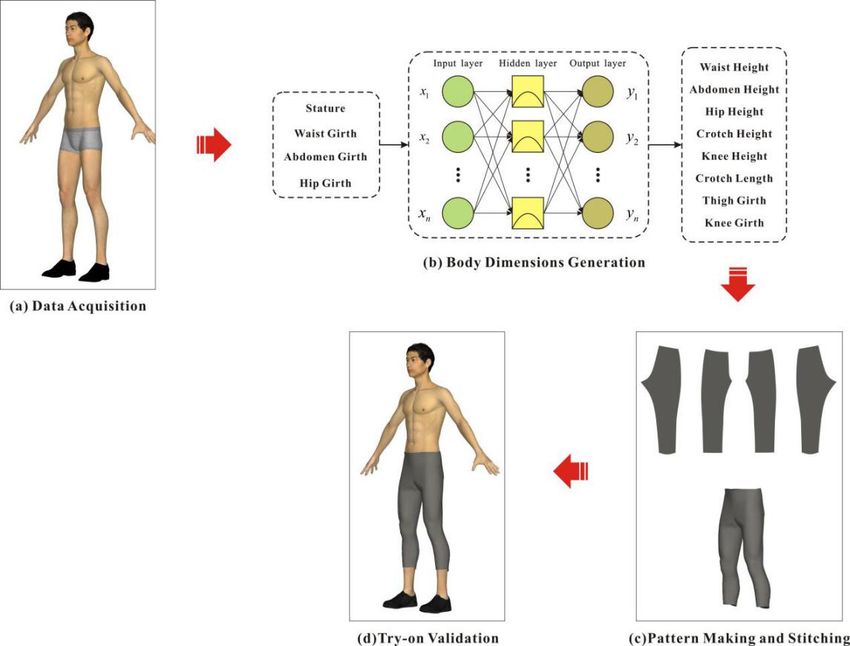
Appl. Sci. 2019, 9, 1140                                                                           2 of 14

wide range of knowledge (e.g., aesthetics, mathematics, ergonomics). The key problem of making
well-fitting garment patterns is to design garment sizes or dimensions, heavily depending on the
expertise and experiences of pattern makers. Generally, the garment sizes are designed and adjusted
by pattern makers according to human body dimensions. Individualized garments need more accurate
human body dimensions. Therefore, anthropometric measurement is an essential prerequisite for
pattern making.
       Currently, shopping over the internet has become more incorporated into people’s lifestyle with
the continuously increasing popularity of the internet. Garment suppliers have been challenged
in providing individualized garments that fit exactly a certain consumer’s body size and body
shape, due to the obstacle of procuring human body dimensions directly and precisely through
the internet. Ordinarily, human body dimensions could be measured manually or automatically.
With the advantages of intuitionistic and convenient tools, manual measurement with tapes has been
applied as a conventional method of human body data acquisition for years. However, since the
method is greatly dependent on the experience and judgement of the measurers, the precision of the
data procured is unreliable, which may easily lead to the problem of poor garment fit. Additionally,
it is also time-consuming. Compared with the manual anthropometric measurement, the efficiency and
accuracy has been greatly improved by 3D human body scanning technology. Over the past decade,
3D human body scanners of various kinds have emerged on the market and been employed in the
apparel industry, such as laser scanning, patterned light projection, stereo photogrammetry, millimeter
waves, and infrared waves [1,2]. Contributing to the development of CCD-chips (Charge-coupled
Device), the 3D body scanners have the advantages of high resolution (1–8 mm) and speed (0.2–3 s),
which makes it possible to collect the whole body’s data precisely and economically [1,2]. However,
since the subjects are required to be naked or wear underwear during the process of body scanning,
numerous consumers refuse to be measured. Some other disadvantages of the devices, including the
bulky design, high price and huge storage capacity for 3D images, have also influenced their further
application in the garment industry, particularly in middle and small-scale garment enterprises [2,3].
Obviously, in the context of sales over the internet, it is unrealistic to utilize the two anthropometric
measurement manners aforementioned [4]. In addition, garment enterprises should meet the
personalized needs for consumers as soon as possible. Therefore, key dimensions (e.g., body height,
bust circumference, waist circumference) which are easy-to-measure are measured physically, while
the other detailed dimensions are calculated by inputting the key dimensions into empirical formulas
based on linear regression (LR) models. For example, the sleeve length could be calculated by inputting
human body height into an LR model. Contributing to inherent simplicity, LR models have been
widely applied in the fields of industrial product design including garments, tools, furniture, and
workplace [5–9]. However, these models are not accurate enough [9]. Thus, it is necessary to develop
an approach of obtaining body dimensions used for garment pattern making faster and more accurate
than the current methods.
       With the rapid development of artificial intelligence (AI) nowadays, predicting human body
dimensions by AI rather than measuring them physically has attracted more and more attention in the
apparel industry. Recently, due to the advantages of artificial neural networks (ANNs), such as good
non-linear approximation abilities and adaptive and self-organizing abilities, and as one of the most
popular machine learning approaches, ANN technology has been widely in many fields, including
viscosity prediction of nanofluid, human behavior prediction, pattern recognition, and adaptive
control [10–14]. In the field of garment pattern making, Chan et al. [15] presented an artificial neural
network model to predict the pattern parameters of men’s shirt in 2003. However, the inputs of the
model proposed consisted of 58 body dimensions which were rather complicated and not easy to collect
simultaneously. In 2014, one study by Zheng Liu et al. [16] put forward a non-linear model to predict
the detailed body sizes using feature parameters extracted by principle component analysis. But the
feature parameters used as the inputs of the proposed model were difficult to calculate in the research.
Another study by Kaixuan Liu et al. [17] in 2017 developed a back propagation (BP) neural networks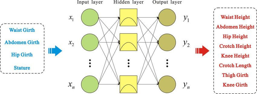
Appl. Sci. 2019, 9, 1140 3 of 14
model to predict lower body dimension used for pants pattern design. However, the application of
other neural networks models was not mentioned in that study. What is more, little attention has been
focused on the application of radial basis function (RBF) ANN in garment pattern making. Therefore,
the aim of this paper is to put forward a new ANN model based on radial basis function to improve the
precision of estimating body dimensions used for garment pattern making. Additionally, the proposed
model could be used for pattern makers with a lack of expertise and experience, through inputting the
learning data based on the knowledge of experienced pattern makers.
The rest of the sections of this study are organized as follows. The “Methodology” section expounds
on the research scheme and procedures in this paper, including anthropometric data acquisition,
and construction of the RBF ANN-based predictive model. In the “Results and Discussion” section,
key factors affecting predictive precision of the proposed model are analyzed and an application of
the model is put forward and in making the patterns of active leggings. Finally, the “Conclusion” is
presented with the conclusions and possible future works.
2. Methodology
2.1. Research Scheme
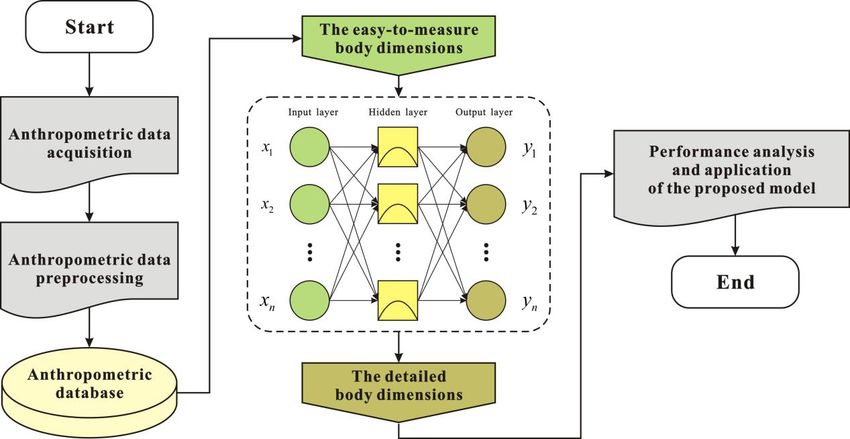
The proposed approach for estimating body dimensions used for garment pattern making is
described in Figure 1. The detailed implementation process is as follows. First, the anthropometric data
of a group of 200 males were gathered to construct the human body dimensions database after data
preprocessing. In the sequential step, the data in the database were divided into two groups: the key
dimensions and the difficult-to-measure detailed dimensions. Then, the ANN predictive models
with different mathematical algorithms were designed, which used the key dimensions as the input
variables and the detailed dimensions needed for garment pattern making as the output variables.
Afterwards, the constructed models were trained and tested by the training dataset and the testing
dataset selected from the database, respectively. Subsequently, the predictive performance of the RBF
ANN model proposed was compared with the BP ANN model and the linear regression model.4 of 15
Appl. Sci. 2019, 9, x FOR PEER REVIEW
Figure 1. Flow chart.
Figure
As a popular Data
2.2. Anthropometric type Acquisition
of clothing,and
tight-fitting activewear without any ease allowance was taken
Preprocessing
as the study sample, in order to verify the performance of the presented model further. The key
body With the advantages
dimensions of a newofsubject
takingwere
automatic
inputtedbody
intomeasurements precisely
the model. Then, within
the body a few seconds,
dimensions related
the VITUS 3D
to making thebody scannerpatterns
activewear was employed to collectby
were estimated the anthropometric
the data
model. Since the of 200 adult
activewear maleswas
selected who
were from the middle and south region of China. The ages of the subjects in this study were between
20 and 48 years of age, and height ranged from 150 to 183 cm.
In the following stage, the data obtained from the 3D scanner were preprocessed by exploratory
analysis. The data preprocessing aimed to figure out the singular values influencing the analysis
results and to investigate the data samples’ distribution. The singular values were mainly induced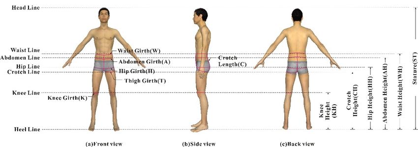
Appl. Sci. 2019, 9, 1140                                                                                                         4 of 14

without any ease allowance, the body dimensions outputted could be utilized as the pattern dimensions.
The activewear patterns were made ultimately based on the estimated body dimensions.

2.2. Anthropometric Data Acquisition and Preprocessing
       With the advantages of taking automatic body measurements precisely within a few seconds,
the VITUS 3D body scanner was employed to collect the anthropometric data of 200 adult males who
were from the middle and south region of China. The ages of the subjects in this study were between
20 and 48 years of age, and height ranged from 150 to 183 cm.
       In the following stage, the data obtained from the 3D scanner were preprocessed by exploratory
analysis. The data preprocessing aimed to figure out the singular values influencing the analysis
results and to investigate the data samples’ distribution. The singular values were mainly induced by
measurement errors and special body types. For the values induced by measurement errors, the data
were re-measured carefully. For the values induced by special body types, all the measurements were
reserved for the following study.
       As an increasingly popular style of clothing, active leggings were taken for instance in this study.
Since active leggings are tight fitting, their pattern dimensions are strongly related to human body
dimensions. Twelve lower-body dimensions related to garment making patterns of active leggings were
selected from the database for further study. Figure 2 illustrates the anthropometric dimensions used
in this study, including stature, waist height, abdomen height, hip height, crotch height, knee height,
waist girth, abdomen girth, hip girth, crotch length, thigh girth, and knee girth. How the dimensions
were measured is explained in Table 1. The subject stood upright and without shoes as shown in
Figure 2 when being measured by the 3D body scanner. Head line was defined as the top of the head,
and the heel line referred to the soles of the feet. The selected anthropometric data were conducted by
Appl. Sci. 2019, analysis
descriptive      9, x FOR PEER
                           andREVIEW
                               the results are given in Table 2.                                    5 of 15

                                   Figure 2.
                                   Figure    Diagram of
                                          2. Diagram of the
                                                         the lower-body
                                                              lower-body dimensions.
                                                                         dimensions.

                   Table 1. Operational definitions of the selected anthropometric measurements.
                   Table 1. Operational definitions of the selected anthropometric measurements.
      No.         Measurements            Abbr.                                   Operational Definitions
    No.        Measurements         Abbr.                             Operational Definitions
      1              Stature              ST         The vertical distance measured from head line to heel line.
     12           Stature
                  Waist Height
                                     ST WHThe vertical    distance    measured from head line to heel line.
                                                     The vertical distance measured from waist line to heel line.
     23        Waist  Height
                 Abdomen  Height     WH AHThe vertical    distance    measured
                                                     The vertical distance measuredfrom
                                                                                      fromwaist   lineline
                                                                                            abdomen       to heel
                                                                                                             to heelline.
                                                                                                                      line.
     34            Hip Height
              Abdomen    Height      AH HHThe vertical
                                                     The vertical
                                                          distancedistance measured
                                                                      measured        from
                                                                                   from     hip line to line
                                                                                          abdomen         heel line.
                                                                                                               to heel line.
      5           Crotch Height           CH         The vertical distance measured from crotch line to heel line.
     46         Hip  Height
                   Knee Height
                                     HH KHThe vertical    distance measured from hip line to heel line.
                                                     The vertical distance measured from knee line to heel line.
     57        Crotch  Height
                   Waist Girth       CH W The vertical    distance    measured
                                                     The length measured   around from    crotch part
                                                                                   the slenderest   lineoftothe
                                                                                                              heel   line.
                                                                                                                 waist  horizontally.
     68          Abdomen
                Knee       Girth
                      Height         KH A The vertical
                                                     The length measured
                                                          distance         around from
                                                                      measured     the fullest
                                                                                          knee part
                                                                                                 lineof the abdomen
                                                                                                         to heel   line.horizontally.
          9          Hip Girth            H          The length measured around the fullest part of the hip horizontally.
                                             The length  measured around the slenderest part of the waist
                                                     The length measured from the center point of front waist line to the
      710        Waist
                  CrotchGirth
                         Length      W C
                                             horizontally.
                                                     center point of back waist line through the crotch.
       11           Thigh Girth            T The length
                                                     The measured
                                                         length measured   around
                                                                       around   thethe  root ofpart
                                                                                     fullest    the thigh
                                                                                                      of thehorizontally.
                                                                                                              abdomen
      812     Abdomen  Girth
                  Knee Girth          A K            The length measured around the knee horizontally.
                                             horizontally.
                                             The length measured around the fullest part of the hip
      9           Hip Girth           H
                                             horizontally.
                                             The length measured from the center point of front waist line to
     10        Crotch Length          C
                                             the center point of back waist line through the crotch.
     11         Thigh Girth           T      The length measured around the root of the thigh horizontally.
     12         Knee Girth            K      The length measured around the knee horizontally.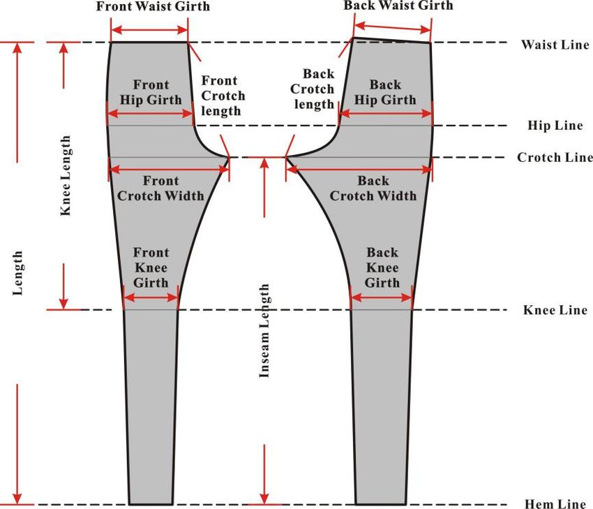
Appl. Sci. 2019, 9, 1140                                                                                      5 of 14

          Table 2. Description of the variables used to construct the radial basis function (RBF) artificial neural
          network (ANN) model.

                 Measurements           Sample Numbers             Mean Value             Standard Deviation
                Stature (cm)                    200                   166.04                       5.32
             Waist Height (cm)                  200                   102.89                       4.31
            Abdomen Height (cm)                 200                   92.32                        4.46
              Hip Height (cm)                   200                    80.15                       3.85
             Crotch Height (cm)                 200                   74.62                        4.10
              Knee Height (cm)                  200                    44.42                       2.35
              Waist Girth (cm)                  200                   79.82                        8.87
            Abdomen Girth (cm)                  200                   82.42                        7.47
               Hip Girth (cm)                   200                    90.65                       5.08
             Crotch Length (cm)                 200                   77.40                        4.73
              Thigh Girth (cm)                  200                   51.62                        3.98
              Knee Girth (cm)                   200                   36.18                        2.08

    2.3. Construction of the RBF ANN Model for Estimating Body Dimensions

    2.3.1. Inputs and Outputs of the RBF ANN Model
           Figure 3 illustrates the flat patterns of active leggings with key structure lines and measurements.
Appl.Compared
      Sci. 2019, 9, with
                    x FORthe anthropometric
                          PEER  REVIEW        measurements shown in Figure 2 and Table 1, the correspondence   6 of 15
    between the key measurements of flat patterns and body dimensions is shown in Table 3. Therefore,
    four body
in Table          dimensions
            3. Therefore,       were
                             four bodyselected for the input
                                         dimensions    were neurons
                                                              selectedof
                                                                       forthe model,
                                                                            the inputwhich were
                                                                                      neurons  ofwaist girth (W),
                                                                                                  the model,  which
wereabdomen
       waist girthgirth(W),
                        (A), hip girth (H),
                             abdomen        and(A),
                                         girth  stature
                                                    hip (ST).
                                                         girth (H), and stature (ST).

                                       Figure
                                        Figure3.3.Flat
                                                   Flat patterns ofactive
                                                        patterns of activeleggings.
                                                                           leggings.

     TheThe   main
           main     objective
                 objective of of
                              thisthis paper
                                    paper    was
                                           was to to construct
                                                   construct ananestimating
                                                                   estimatingmodel
                                                                               modelfor
                                                                                     forpattern
                                                                                         patternmaking.
                                                                                                  making. For
the For the model,
    model,         the inputs
             the inputs  werewere   easy-to-measure
                               easy-to-measure       bodydimensions,
                                                  body    dimensions, and
                                                                       and the
                                                                            theoutputs
                                                                                outputswere
                                                                                        weredetailed body
                                                                                              detailed  body
    dimensions. As a kind of tight-fitted garment, the patterns of active leggings studied in this paper
dimensions. As a kind of tight-fitted garment, the patterns of active leggings studied in this paper
    were without any ease allowance and the body dimensions outputted by the models could be utilized
were without any ease allowance and the body dimensions outputted by the models could be utilized
    as the pattern dimensions. Thus, eight body dimensions were chosen for the output neurons of the
as the pattern dimensions. Thus, eight body dimensions were chosen for the output neurons of the
models, including waist height (WH), abdominal height (AH), hip height (HH), crotch height (CH),
knee height (KH), crotch length (C), thigh girth (T), and knee girth (K).

         Table 3. Correspondence between the key measurements of flat patterns and body dimensions.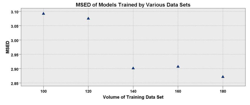
Appl. Sci. 2019, 9, 1140                                                                                         6 of 14

models, including waist height (WH), abdominal height (AH), hip height (HH), crotch height (CH),
knee height (KH), crotch length (C), thigh girth (T), and knee girth (K).

          Table 3. Correspondence between the key measurements of flat patterns and body dimensions.

                                          Key Measurements of Flat Patterns
                 No                                                                          Body Dimensions
                                           Front                       Back
                  1                  Front Waist Girth            Back Waist Girth                 W
                  2                   Front Hip Girth             Back Waist Girth                 H
                  3                 Front Crotch Width           Back Crotch Width                 T
                  4                  Front Knee Girth             Back Knee Girth                  K
                  5                                      Length                                   WH
                  6                                   Knee Length                                WH, KH
                  7                                  Inseam Length                                CH

      The architecture of the predictive model proposed in this study is shown in Figure 4. The model
based on the RBF ANN had three layers, which were one input layer with four neurons, one output
layer with eight neurons, and one hidden layer. The four neurons in the input layer were
the easy-to-measure key dimensions, such as waist girth, abdomen girth, hip girth, and stature.
The eight neurons in the output layer were the detailed body dimensions, including waist height,
abdomen      height, hip height, crotch height, knee height, crotch length, thigh girth, and knee girth.
Appl. Sci. 2019, 9, x FOR PEER REVIEW                                                                7 of 15

      Figure 4.4.Architecture
                  Architectureof of
                                 the the  radial
                                      radial basisbasis function
                                                  function       (RBF) artificial
                                                           (RBF) artificial         neural networks
                                                                            neural networks (ANN) for(ANN)    for
                                                                                                      estimating
      estimating
      body        body dimensions.
           dimensions.

2.3.2. Training Dataset
2.3.2. Training Dataset and
                        and Testing
                            TestingDataset
                                    Dataset
     Table
     Table 44 shows
               showsthe
                     thedataset
                         datasetused
                                  usedin in
                                         thisthis study,
                                              study,      including
                                                      including     training
                                                                training      dataset
                                                                         dataset      and testing
                                                                                 and testing       dataset.
                                                                                             dataset. Since
Since the sample  size was too large, only   part of the data are shown  in
the sample size was too large, only part of the data are shown in Table 4.  Table 4.

                           Table 4. Parts of the data used to construct RBF ANN model (unit: cm).
                           Table 4. Parts of the data used to construct RBF ANN model (unit: cm).
                        Input
                         InputData
                               Data                                           Output Data
                                                                              Output Data
   SN
    SN        W          A      H          ST       WH        AH      HH      CH      KH         C       T        K
               W          A      H          ST        WH        AH     HH      CH     KH         C      T       K
    1        85.2      85.3    89.8       157.0      97.5     89.4    78.4    71.1   42.5       72.3    52.5    35.2
    21       75.0      83.2    86.4       161.1     101.6     90.4    78.2    72.3   43.1       75.8    46.8    34.9
              85.2      85.3    89.8       157.0       97.5    89.4    78.4    71.1   42.5      72.3   52.5    35.2
    3        80.9      81.0    90.3       164.9      99.3     92.7    78.6    72.1   42.1       75.5    50.5    37.0
    42       88.0
              75.0     89.8
                        83.2   97.4
                                86.4      169.5
                                           161.1    106.8
                                                      101.6   94.0
                                                               90.4   79.8
                                                                       78.2   75.6
                                                                               72.3  41.9
                                                                                      43.1      81.9
                                                                                                75.8    57.2
                                                                                                       46.8     38.8
                                                                                                               34.9
    5        79.7      78.5    90.7       163.9     101.4     91.3    78.4    73.7   44.4       74.8    51.7    35.9
    63       73.9
              80.9     75.7
                        81.0   87.2
                                90.3      161.7
                                           164.9    100.4
                                                       99.3   91.7
                                                               92.7   76.8
                                                                       78.6   71.0
                                                                               72.1  42.7
                                                                                      42.1      75.5
                                                                                                75.5    51.9
                                                                                                       50.5     35.3
                                                                                                               37.0
    7        89.0      87.8    99.3       174.0     108.6     99.3    89.0    82.2   50.1       74.0    56.2    41.4
      4       88.0      89.8    97.4       169.5      106.8    94.0    79.8    75.6   41.9      81.9   57.2    38.8
      5       79.7         78.5    90.7     163.9    101.4     91.3    78.4    73.7   44.4      74.8   51.7    35.9
      6       73.9         75.7    87.2     161.7    100.4     91.7    76.8    71.0   42.7      75.5   51.9    35.3
      7       89.0         87.8    99.3     174.0    108.6     99.3    89.0    82.2   50.1      74.0   56.2    41.4
      8
Appl. Sci. 2019, 9, 1140 7 of 14
Table 4. Cont.
Input Data Output Data
SN
W A H ST WH AH HH CH KH C T K
8 82.7 80.9 90.3 169.4 100.7 91.4 78.7 71.0 45.9 74.5 54.3 36.6
9 74.5 86.3 91.9 176.0 109.4 85.0 84.2 79.3 51.3 79.6 50.3 36.6
10 80.6 84.3 90.3 171.1 105.5 97.0 82.2 77.9 47.1 79.2 51.4 36.4
11 88.5 87.6 91.6 163.6 101.3 89.8 80.3 73.6 45.6 75.7 51.3 36.4
12 92.1 95.4 95.4 166.0 104.3 96.8 78.8 73.3 42.7 84.0 53.4 37.7
13 77.9 78.6 85.2 165.2 104.5 97.2 76.5 73.4 44.0 79.0 46.4 35.2
14 87.1 87.6 91.6 166.3 100.8 90.3 80.0 70.3 43.3 80.9 52.8 37.5
15 75.5 81.0 92.4 173.1 108.9 98.4 83.6 79.5 48.0 79.7 51.2 37.3
16 80.3 87.3 94.5 175.6 108.3 98.0 83.3 79.2 50.4 80.2 55.4 37.2
17 71.0 72.8 83.8 156.3 97.0 80.3 74.0 70.0 42.0 71.5 50.9 37.1
18 74.7 82.3 87.2 159.0 96.4 84.3 74.5 69.4 41.5 73.9 49.8 34.4
19 92.8 97.3 96.0 164.1 100.2 86.9 78.3 71.5 42.3 82.4 56.6 38.2
20 82.9 83.5 90.9 183.2 116.4 104.4 92.2 90.0 53.2 79.9 54.4 36.2
Note: SN is sample number. For W, A, H, ST, WH, AH, HH, CH, C, T, K, please refer to Figure 2 and Table 1.
2.4. Simulation of RBF ANN Model for Estimating Body Dimensions
The radical basic function (RBF) ANN is one of the feedforward neural networks with simple
structure and has the advantages of approximating any non-linear function with arbitrary accuracy
and fast convergence [16,18]. Therefore, the predictive model proposed in this study was constructed
based on RBF ANN with the architecture composed of an input layer, hidden layer, and output layer.
In this paper, the simulation process included eight steps as follows.
Step 1: Distributed the element of X = [x(1), x(2), . . . , x(p)]T to the input layer. Where, X was a
matrix of inputting samples; p was the number of input samples.
Step 2: Calculated the inputs of the hidden layer;
n
hi j (k) = ∑ wij xi (k), j = 1, 2, . . . , h (1)
1
where, hij (k) was the inputs of the kth inputting sample in the jth node of hidden layer, k = 1, 2, . . . ,
p; wij was the linkage weights between input layer and hidden layer. For the RBF ANN, the linkage
weights between the input layer and the hidden layer were set to 1.
Step 3: Calculated the cluster centers {c1 , c2 , . . . , ch } and the parameter σ in the hidden layer;
For the RBF ANN, the outputs of the hidden layer were activated by a radial Gauss function G:
k x ( k ) − ci k
G ( x (k ), ci ) = exp − , i = 1, 2, . . . , h (2)
2σ2
where, ci was the ith cluster center in the hidden layer; σ, also known as spread, was the smoothing
parameter, k·k was the representative of the Euclidean norm. Thus, the cluster centers {c1 , c2 , . . . ,
ch } and the parameter σ was set to 1.0 initially in this study. The cluster centers {c1 , c2 , . . . , ch } were
determined by the K-means algorithm. The operational procedures were as follows:
(1) An initial set of cluster centers {c1 , c2 , . . . , ch } was chosen from the inputs of hidden
layer randomly;
(2) Each of the input of hidden layer was assigned to its closest cluster center according to the
Euclidean metrics;
(3) New cluster centers were computed as the means of the Kth cluster;
(4) If the position of any cluster center changed, return to (2), otherwise, stop.Appl. Sci. 2019, 9, 1140 8 of 14
Step 4: Calculated the outputs of the hidden layer;
The outputs of hidden layer were calculated based on a radial Gauss function G shown as
Formula (2).
k x (k) − c j k
ho j (k) = exp − , j = 1, 2, . . . , h (3)
2σ2
where, hoj (k) was the outputs of the kth inputting sample in the jth node of the hidden layer.
Step 5: Calculated the inputs and outputs of the output layer;
h
yio (k) = ∑ wio ho j (k), o = 1, 2, . . . , m (4)
1
yoo (k) = f (yio (k)) (5)
where, yio (k) was the inputs of the kth inputting sample in the oth node of the output layer; yoo (k)
referred to the output of the kth inputting sample in the oth node of the output layer; wio was the linkage
weights between the hidden layer and the output layer; f (·) was the activation function in the output
layer and the Sigmoid function was used as the activation function in this study. Thus, the outputs of
the output layer could be calculated:
1
f (yio (k )) = (6)
1 + e−yio (k)
Step 6: Updated the linkage weights between the hidden layer and the output layer.
The linkage weights between the hidden layer and the output layer were amended according to
Formulas (8) and (9).
N +1 N N
wio = αwio + ∆wio (7)
∂E
∆wio = −η (8)
∂wio
where, α referred to the momentum factor, α and η referred to the learning speed, and both of them
could accelerate the convergence rate of RBF ANN. The initial value of parameter α was set to 0.9 and
η was adaptive in this study.
Step 7: Calculated global error EG .
p
EG = ∑ Ei (9)
1
m
1 2
where, E = 2 ∑[do (k) − yo (k)] was the cost function to measure errors.
1
Step 8: Checked whether the error of the model met the goals.
If either the error was acceptably small or other terminating conditions occurred, the model
stopped. Else, return to step 2 for the next round of learning until the goals were reached.
3. Results and Discussion
In order to reveal the effects of the factors affecting the estimating performance of the models,
including volume of training dataset, quantity of hidden neurons, parameter σ in the hidden layer,
and momentum factor α, a series of experiments were conducted. Various models were tested by the
same dataset randomly extracted from the dataset illustrated in Table 4. The testing dataset in this
study in shown in Table 5.Appl. Sci. 2019, 9, 1140 9 of 14
Table 5. Testing dataset (unit: cm).
Input Data Expected Output Data
SN
W A H ST WH AH HH CH KH C T K
1 101.9 101.9 102.5 164.0 103.1 90.3 80.7 74.3 43.2 84.0 58.9 36.8
2 69.2 74.7 91.1 174.6 108.4 97.7 83.7 82.0 46.4 74.1 51.2 35.7
3 85.5 86.0 93.4 159.6 101.2 90.8 76.9 70.3 42.7 84.6 55.1 35.4
4 85.5 90.1 95.9 158.3 96.6 83.7 74.1 67.9 40.1 77.0 55.0 34.0
5 64.3 70.1 80.6 163.3 101.1 90.3 77.5 75.2 42.5 73.4 43.7 33.1
6 71.6 76.1 86.9 161.3 97.3 85.8 76.3 71.6 41.2 71.9 50.7 34.7
7 64.3 72.5 79.3 164.3 101.8 92.6 79.2 75.6 43.9 69.2 42.9 33.1
8 72.5 77.5 87.7 171.0 106.9 94.3 81.1 77.9 46.6 72.0 48.4 34.1
9 93.9 95.4 94.5 160.7 101.9 89.6 80.5 75.3 43.6 74.5 52.0 37.2
10 96.0 94.7 100.3 168.8 104.3 92.5 81.6 77.4 44.8 80.0 57.0 38.4
11 86.1 89.2 95.9 166.2 100.4 88.6 74.6 69.7 41.1 85.3 55.9 38.6
12 72.4 76.4 90.9 173.2 108.7 99.5 85.7 80.6 47.3 72.2 49.7 35.0
13 80.0 80.5 87.9 167.3 106.3 96.2 84.0 78.5 44.5 65.5 50.4 35.2
14 72.9 78.3 89.1 174.7 97.0 83.8 83.0 79.7 46.8 76.0 49.2 37.0
15 78.4 78.9 88.1 167.5 101.3 92.1 81.6 76.8 44.3 71.9 52.3 36.2
16 68.0 71.0 82.4 168.3 103.6 96.1 82.6 77.5 45.3 65.8 45.6 32.8
17 75.8 81.3 95.6 172.7 107.7 98.3 86.3 81.4 47.0 73.8 55.8 35.6
18 74.7 81.0 92.2 171.2 109.0 93.2 81.7 76.7 45.1 81.8 53.8 37.4
19 61.4 63.2 79.2 165.6 101.9 92.0 79.6 76.9 44.5 70.0 43.7 31.8
20 71.2 76.5 89.5 169.7 103.3 92.5 81.3 75.4 44.5 76.2 52.2 36.0
Note: SN is testing sample number. For W, A, H, ST, WH, AH, HH, CH, C, T, K, please refer to Figure 2 and Table 1.
After the model was tested, dij were calculated according to Formula (10), which was defined as
the absolute deviation between Yij and Y’ij . D was defined as a matrix composed of dij according to
formula (11). MSED referred to mean square error of D, which was utilized to evaluate the predictive
precision of the models.
dij = Yij − Yij0 , i = 1, 2, . . . , 20, j = 1, 2, . . . , 8 (10)
· · · d1j
d11
.. .. .. , i = 1, 2, . . . , 20, j = 1, 2, . . . , 8
D= . . . (11)
di1 · · · dij
where, Yij and Y’ij were respectively defined as the estimated output data and the expected output
data of the ith inputting sample in the jth node of output layer.
3.1. Effects of Volume of Training Dataset
Since the training dataset was one of the key factors affecting the performance of the RBF
ANN model, five various training datasets with 100, 120, 140, 160, and 180 samples, respectively,
were established in order to investigate the effects. For each training dataset, the data were extracted
randomly from the remaining data in the dataset shown in Table 4. Then, an RBF ANN model with
4 input neurons, 20 hidden neurons, and 8 output neurons were trained by the five sets, respectively,
using the same parameter σ (σ = 1.0) in the hidden layer and momentum factor α (α = 0.9). After being
well-trained, the five models were tested by the datasets shown in Table 5.
Figure 5 illustrates the MSED of the five models. It can be easily seen that the MSE dropped as the
volume of training datasets increased from 100 to 180. Among the five models, the MSED of the model
trained by 180 samples was the lowest. From the perspective of MSED, the precision of the models
grew with the increase in training samples. It means that the more trained data the models learned,
the stronger were their estimating ability.Appl. Sci. 2019, 9, x FOR PEER REVIEW 11 of 15
the model trained by 180 samples was the lowest. From the perspective of MSED, the precision
of the models grew with the increase in training samples. It means that the more trained10data
Appl. Sci. 2019, 9, 1140 of 14
the models learned, the stronger were their estimating ability.
Figure 5. Mean square error of D (MSED) of the RBF ANN models trained by datasets with
Figure
various5.volumes.
Mean square error of D (MSED) of the RBF ANN models trained by datasets with various
volumes.
3.2. Effects of the Quantity of Hidden Neurons
3.2. Effects of the Quantity of Hidden Neurons
Quantity of neurons in the hidden layer had great impact on the performance of the RBF ANN.
Quantity
Generally, theofprecision
neurons of in the hidden
RBF ANN layercould
had great impact on
be improved asthe
theperformance
quantity of of thethe RBF ANN.
hidden layer
Generally, the precision
increased. However, of the neurons
too many RBF ANN could
in the be improved
hidden layer willas the quantity
prolong of the hidden
the convergence layer
rate of the
increased.
RBF ANN,However,
and even leadtoo many neurons
to failure in the
to train the hidden
model. layer willtoprolong
In order the the
determine convergence rate of the
optimum number of
RBF
hiddenANN, and even
neurons, lead to
multiple failure to train
experiments werethe model. Twelve
executed. In orderRBFto determine
ANN models the optimum number
with various hiddenof
hidden neurons,
layer were multiple
constructed experiments
firstly. wereof
The quantity executed. Twelve RBF
hidden neurons wereANN models
60, 65, 70, 71,with various
72, 73, 75, 80,hidden
85, 90,
layer
95, andwere
100,constructed
respectively. firstly. The quantity
The parameter of hidden
σ and neurons
α were still set towere 60, 0.9.
1.0 and 65, 70, 71, 72, 73,the
Afterwards, 75, twelve
80, 85,
90, 95, and
models were100, respectively.
trained by the same Thedataset
parameter
with σ180and α wereFinally,
samples. still setthey
to 1.0
wereand 0.9. Afterwards,
tested with the datasetthe
twelve
in Tablemodels
5. were trained by the same dataset with 180 samples. Finally, they were tested with the
dataset
TheinMSED
Table 5.of the models with various hidden layers are shown in Table 6. When the quantity
of the hidden neurons increased from 60 to 72, the MSED declined gradually, while rising gradually
The MSED of the models with various hidden layers are shown in Table 6. When the quantity of
as the quantity of the hidden neurons increased from 72 to 90. From 90 to 100, the MSED descended
the hidden neurons increased from 60 to 72, the MSED declined gradually, while rising gradually as
again. Overall, the MSED of the model with 72 hidden neurons has the minimum value relatively.
the quantity of the hidden neurons increased from 72 to 90. From 90 to 100, the MSED descended
Therefore, it could be considered that the precision of the RBF ANN model reached its maximum when
again. Overall, the MSED of the model with 72 hidden neurons has the minimum value relatively.
the quantity of neurons in the hidden layer was 72.
Therefore, it could be considered that the precision of the RBF ANN model reached its maximum
when the quantity Tableof6.neurons
Mean squarein the hidden
error layer was
of D (MSED) 72.
of models with various hidden layers.
Table Model
6. MeanNo. Number
square error of Hidden
of D (MSED) Neurons
of models with variousMSED
hidden layers.
Model No.1 60
Number of Hidden
2.8904
2 65 Neurons MSED
2.8521
1 3 70 2.8351
4 6071 2.8904
2.8528
2 5 72 2.8055
65 2.8521
6 73 2.8284
3 7 7075 2.8306
2.8351
8 80 2.8409
4 9 7185 2.8454
2.8528
10 90 2.8919
5 7295 2.8055
11 2.8708
6 12 100 2.8386
73 2.8284
7
3.3. Effects of the Parameter σ in the Hidden Layer 75 2.8306
In the hidden layer of the RBF ANN, since the outputs were activated by Formula (2),
the parameter σ should have influenced the estimating performance. Based on the findings of
Sections 3.1 and 3.2, thirteen RBF ANN models with four inputs, 72 hidden neurons, and eight outputsAppl. Sci. 2019, 9, 1140 11 of 14
were built for further study. The only difference among them was the parameter σ, which were 0.001,
0.005, 0.008, 0.01, 0.011, 0.012, 0.013, 0.015, 1, 1.25, 1.67, 2.5, and 5, respectively. After being well-trained
and tested, the models were compared according to MSED. Table 7 shows the MSED of the thirteen
models. As σ altered from 0.001 to 5, the MSED presented a tendency to descend first and then rise.
When σ was at 0.012, MSED came to the minimum. Thus, the optimum value of σ was determined.
Table 7. The MSED of the models with various parameters of σ in the hidden layer.
Model No. Parameter σ MSED
1 0.001 2.7423
2 0.005 2.7395
3 0.008 2.7293
4 0.010 2.7283
5 0.011 2.7280
6 0.012 2.7279
7 0.013 2.7284
8 0.015 2.7292
9 1.000 2.8055
10 1.250 2.9829
11 1.670 2.9254
12 2.500 3.0759
13 5.000 3.4778
3.4. Effects of the Momentum Factor α
In order to find how the momentum factor affected the RBF ANN model in this study, ten kinds of
α were selected between 0.1 and 1, and they were 0.1, 0.2, 0.3, 0.4, 0.5, 0.6, 0.7, 0.8, 0.9, and 1. The RBF
ANN model constructed based on the findings of Section 3.3 were trained ten times according to the α
selected. Although the α was changing, MSED was almost invariant. The running time of the model
expended gradually with the increase of α.
3.5. Comparison with Linear Regression Model and BP ANN Model
Table 8 shows the MSED of three predictive models, which were the RBF ANN model with the
optimum performance constructed in this study, the BP ANN model, and the linear regression model.
For each anthropometric measurement, the MSED of RBF ANN model was less than that of the other
two models, which meant that the estimating performance of the RBF ANN model was better than
the others.
Table 8. The MSED of various predictive models.
MSED
Measurements
RBF ANN Model BP ANN Model Linear Regression Model
Waist Height 3.0814 3.1185 3.1854
Abdomen Height 3.0197 3.7809 3.7631
Hip Height 1.8514 2.0029 2.0887
Crotch Height 1.0450 1.1139 2.0705
Knee Height 1.9307 2.0918 2.0084
Crotch Length 3.9251 4.0531 5.9871
Thigh Girth 1.4631 1.7397 2.5929
Knee Girth 1.0238 1.1137 1.4043
3.6. Application of the Body Dimensions Estimated by RBF ANN Model
In order to verify the model presented in this study, tight-fitted active leggings patterns making
was taken for use as a case study. Due to tight fitness, the outputted body dimensions could be used as
pattern dimensions of active leggings.Appl. Sci. 2019, 9, 1140 12 of 14
The application process in this study in illustrated in Figure 6, as follows:
Initially, anthropometric data of a subject were selected randomly. The subject’s stature was
171.8 cm, waist girth was 68.9 cm, abdomen girth was 77.2 cm, and hip girth was 88.9 cm. Therefore,
the input vector x = (171.8, 68.9, 77.2, 88.9). The desired output vector d = (105.8, 94.7, 82.8, 77.4,
45.2, 77.2, 49.2, 35.4) was composed of the real dimensions of the subject, which represented waist
height, abdomen height, hip height, crotch height, knee height, crotch length, thigh girth, and knee
girth, respectively.
Secondly, the RBF ANN was utilized to estimate the body dimensions related to making the
patterns of active leggings. After the vector d was inputted into the predictive model based on RBF
ANN, the output vector y was generated, as follows:
y = (106, 94.1, 83.2, 77.6, 45.9, 74.9, 48.8, 35.2)
Sequentially, the body dimensions generated by the RBF ANN model were employed to making
the patterns of active leggings. Then, the patterns were joined together into 3D active leggings by
virtual stitching technology.
Finally, the stitched leggings were tried on by a virtual avatar to evaluate the fitness.
The available evidence lent support to the view that the proposed RBF ANN model could estimate
the body dimensions related to active leggings pattern making efficiently and precisely. The predictive
accuracy would be further improved by more training data.
Appl. Sci. 2019, 9, x FOR PEER REVIEW 14 of 15
predictive model
Figure 6. Application of the body dimensions predictive model based
based on
on RBF
RBF ANN.
ANN.
4.
4. Conclusions
Conclusions
In
In order
order to
to meet
meet the
the personalized
personalized requirements
requirements of of consumers
consumers in in the
the internet
internet era,
era, this
this study
study has
has
proposed a new neural networks method based on RBF ANN for garment pattern
proposed a new neural networks method based on RBF ANN for garment pattern making, especiallymaking, especially
for tight-fitted garments,
for tight-fitted garments,which
whichisisless
less time-consuming
time-consuming andand more
more accurate
accurate thanthan current
current methods.
methods. The
The key factors affecting the models, such as volume of the training dataset, quantity
key factors affecting the models, such as volume of the training dataset, quantity of hidden neurons, of hidden
neurons,
spreading spreading
parameterparameter σ, and momentum
σ, and momentum factor
factor α, were were analyzed.
α, analyzed. AfterAfter multiple
multiple experiments,
experiments, the
optimum parameters were determined. When spreading parameter σ and momentum factor α were
set to 0.012 and 1, the RBF ANN model with four inputs, 72 hidden neurons, and eight outputs could
reach the maximum accuracy, after being trained by the dataset with 180 samples. Compared with
the traditional linear regression model used in the apparel industry, the RBF ANN model was
superior on predictive precision contributing to its outstanding non-linear mapping capacity. TheAppl. Sci. 2019, 9, 1140 13 of 14
the optimum parameters were determined. When spreading parameter σ and momentum factor α were
set to 0.012 and 1, the RBF ANN model with four inputs, 72 hidden neurons, and eight outputs could
reach the maximum accuracy, after being trained by the dataset with 180 samples. Compared with the
traditional linear regression model used in the apparel industry, the RBF ANN model was superior
on predictive precision contributing to its outstanding non-linear mapping capacity. The proposed
RBF ANN model had a simpler structure with higher estimating accuracy than the BP ANN model.
With the approaching digital customization era in the apparel industry, it is feasible to adopt the RBF
ANN model proposed in this study for a computer-aided body dimension auto-generation system,
which could promote the accuracy and efficiency of pattern designers and improve the fitness of
garments significantly.
Since the presented RBF ANN model in this study was trained by a dataset consisting of
200 subjects only, the accuracy of the model could be further improved. Apart from the sample
capacity, the factors influencing body dimensions such as age, race, and geographical areas should be
considered in future work. Although the approach proposed in this study was concentrated on making
tight fitting garment patterns like active leggings, and it could also be applied in pattern dimension
prediction of other garments with different fitness. In the future, through inputting more learning data
from experienced pattern makers, the proposed model could be used by pattern makers lacking in
related expertise and experience.
Author Contributions: Conceptualization, Z.W. and J.W.; Methodology, Z.W. and Y.X.; Funding acquisition, Z.W.,
Y.X. and K.L.; Supervision, J.W.; Validation, Z.W., Y.X. and Y.Y.; Writing-original draft, Z.W.
Funding: This research was funded by the key Research Project of Humanities and Social Sciences in Anhui
Province College (grant number SK2016A0116 and SK2017A0119), the Open Project Program of Anhui Province
College of Anhui Province College Key Laboratory of Textile Fabrics, Anhui Engineering and Technology Research
Center of Textile (grant number 2018AKLTF15), the Humanities and Social Sciences Research Project of higher
Education Promotion Program in Anhui Province College (grant number TSSK2016B20), the National Natural
Science Foundation of China (grant number 61806161) and Special Scientific Research Plan Projects of Shaanxi
Education Department (grant number 18JK0352).
Conflicts of Interest: The authors declare no conflict of interest.
References
1. Daanen, H.M.; Van De Water, G.J. Whole body scanners. Displays 1998, 19, 111–120. [CrossRef]
2. Daanen, H.A.M.; Ter Haar, F.B. 3D whole body scanners revisited. Displays 2013, 34, 270–275. [CrossRef]
3. Uhm, T.; Park, H.; Park, J.-I. Fully vision-based automatic human body measurement system for apparel
application. Measurement 2015, 61, 169–179. [CrossRef]
4. Wu, G.; Liu, S.; Wu, X.; Ding, X. Research on lower body shape of late pregnant women in Shanghai area of
China. Int. J. Ind. Ergon. 2015, 46, 69–75. [CrossRef]
5. Lacko, D.; Huysmans, T.; Vleugels, J.; de Bruyne, G.; van Hulle, M.M.; Sijbers, J.; Verwulgen, S. Product
sizing with 3D anthropometry and k-medoids clustering. Comput.-Aided Des. 2017, 91, 60–74. [CrossRef]
6. Agha, S.R.; Alnahhal, M.J. Neural network and multiple linear regression to predict school children
dimensions for ergonomic school furniture design. Appl. Ergon. 2012, 43, 979–984. [CrossRef] [PubMed]
7. Chan, A.P.; Fan, J.; Yu, W.M. Prediction of men’s shirt pattern based on 3D body measurements. Int. J. Cloth.
Sci. Technol. 2005, 17, 100–108. [CrossRef]
8. Ngassa, C.N.; Akanbi, O.G.; Ismaila, S.O. Models for estimating the anthropometric dimensions using
standing height for furniture design. Eur. J. Mark. 2014, 12, 336–347.
9. Poirson, E.; Parkinson, M. Estimated anthropometry for male commercial pilots in Europe and an approach
to its use in seat design. Int. J. Ind. Ergon. 2014, 44, 769–776. [CrossRef]
10. Zhao, N.; Li, Z. Viscosity Prediction of Different Ethylene Glycol/Water Based Nanofluids Using a RBF
Neural Network. Appl. Sci. 2017, 7, 409. [CrossRef]
11. Almeida, A.; Azkune, G. Predicting Human Behaviour with Recurrent Neural Networks. Appl. Sci. 2018, 8,
305. [CrossRef]
12. Liu, Y.; Zhao, J.; Xiao, Y. C-RBFNN: A user retweet behavior prediction method for hotspot topics based on
improved RBF neural network. Neurocomputing 2018, 275, 733–746. [CrossRef]Appl. Sci. 2019, 9, 1140 14 of 14
13. Shi, X.; Cheng, Y.; Yin, C.; Huang, X.; Zhong, S. Design of adaptive backstepping dynamic surface control
method with RBF neural network for uncertain nonlinear system. Neurocomputing 2018, 330, 490–503.
[CrossRef]
14. Zhang, X.; Sun, S.; Li, C.; Tang, Z. Impact of Load Variation on the Accuracy of Gait Recognition from Surface
EMG Signals. Appl. Sci. 2018, 8, 1462. [CrossRef]
15. Chan, A.P.; Fan, J.; Yu, W. Men’s Shirt Pattern Design Part II: Prediction of Pattern Parameters from 3D Body
Measurements. FIBER 2003, 59, 328–333. [CrossRef]
16. Liu, Z.; Li, J.; Chen, G.; Lu, G. Predicting detailed body sizes by feature parameters. Int. J. Cloth. Sci. Technol.
2014, 26, 118–130. [CrossRef]
17. Liu, K.; Wang, J.; Kamalha, E.; Li, V.; Zeng, X. Construction of a prediction model for body dimensions
used in garment pattern making based on anthropometric data learning. J. Text. Inst. 2017, 108, 2107–2114.
[CrossRef]
18. Meyer-Baese, A.; Schmid, V. Chapter 7—Foundations of Neural Networks. In Pattern Recognition and Signal
Analysis in Medical Imaging, 2nd ed.; Meyer-Baese, A., Schmid, V., Eds.; Academic Press: Oxford, UK, 2014;
pp. 197–243.
© 2019 by the authors. Licensee MDPI, Basel, Switzerland. This article is an open access
article distributed under the terms and conditions of the Creative Commons Attribution
(CC BY) license (http://creativecommons.org/licenses/by/4.0/).You can also read