Estimating road transport costs between EU regions - JRC TECHNICAL REPORT JRC Working Papers on Territorial Modelling and Analysis No 04/2019

JRC TECHNICAL REPORT

 Estimating road transport
 costs between EU regions
 JRC Working Papers on
 Territorial Modelling and Analysis
 No 04/2019

Authors:
Persyn, D.,
Díaz-Lanchas, J.,
Barbero, J.

2019 Joint
 Research
 Centre

This publication is a Technical report by the Joint Research Centre (JRC), the European Commission’s science and knowledge service. It
aims to provide evidence-based scientific support to the European policymaking process. The scientific output expressed does not imply a
policy position of the European Commission. Neither the European Commission nor any person acting on behalf of the Commission is
responsible for the use that might be made of this publication. For information on the methodology and quality underlying the data used
in this publication for which the source is neither Eurostat nor other Commission services, users should contact the referenced source. The
designations employed and the presentation of material on the maps do not imply the expression of any opinion whatsoever on the part
of the European Union concerning the legal status of any country, territory, city or area or of its authorities, or concerning the delimitation
of its frontiers or boundaries.

Contact information
Name: Simone Salotti
Address: Edificio Expo, C/Inca Garcilaso 3, 41092 Sevilla (Spain)
Email: simone.salotti@ec.europa.eu
Tel.: +34 954488250

EU Science Hub
https://ec.europa.eu/jrc

JRC114409

Seville: European Commission, 2019

© European Union, 2019

The reuse policy of the European Commission is implemented by the Commission Decision 2011/833/EU of 12 December 2011 on the
reuse of Commission documents (OJ L 330, 14.12.2011, p. 39). Except otherwise noted, the reuse of this document is authorised under
the Creative Commons Attribution 4.0 International (CC BY 4.0) licence (https://creativecommons.org/licenses/by/4.0/). This means that
reuse is allowed provided appropriate credit is given and any changes are indicated. For any use or reproduction of photos or other
material that is not owned by the EU, permission must be sought directly from the copyright holders.

All content © European Union, 2019 (unless otherwise specified)

How to cite this report: Persyn, D., Díaz-Lanchas, J., and Barbero, J. (2019). Estimating road transport costs between EU regions. JRC
Working Papers on Territorial Modelling and Analysis No. 04/2019, European Commission, Seville, JRC114409.
The JRC Working Papers on Territorial Modelling and Analysis are published under the supervision of Simone Salotti and Andrea
Conte of JRC Seville, European Commission. This series mainly addresses the economic analysis related to the regional and territorial
policies carried out in the European Union. The Working Papers of the series are mainly targeted to policy analysts and to the academic
community and are to be considered as early-stage scientific papers containing relevant policy implications. They are meant to
communicate to a broad audience preliminary research findings and to generate a debate and attract feedback for further improvements.

Acknowledgements
This paper greatly benefitted from the technical assistance on the computational aspects
provided by Andris Peize and Alfredo Peña Palma, and valuable comments by Aris
Christodoulou, Panayotis Christidis, Ana Margarida Condeço-Melhorado, José L. Zofío,
and Simone Salotti. We are grateful for comments provided by participants in the 58th
ERSA Congress in Cork (Ireland), the VI Regional Modelling Workshop in Seville (Spain),
and the XLVI International Conference on Regional Science in Valencia (Spain).

Abstract
Transport costs are a crucial element of any spatial economic model. Surprisingly, good
transport cost estimates at a detailed spatial level for the EU are not readily available. In
this paper we address this issue by estimating a novel dataset of road freight transport
costs for goods for the EU regions at the NUTS 2 level. In the spirit of the generalized
transport cost (GTC) concept, we calculate the composite cost related to distance and
time for the optimal route of a representative truck. We consider routes between large
random samples of centroids drawn from a 1kmx1km population density grid. These
transport costs are averaged to obtain an origin-destination cost matrix (in euros) at the
region-pair level. The sampling approach also allows calculating the average transport
cost within the regions. We separately report the corresponding iceberg transport costs
for each pair of European regions, since this is the form of input required by many
economic models. We also consider the effect of changes in the components of the GTC
in order to evaluate transport policies. We set up a transport policy tool to assess the
impact of road-transport infrastructure investment in a region by considering upgrading
roads to highways. We apply this tool to study transport infrastructure investment
through the European Cohesion Policy program 2014-2020.

Estimating road transport costs between EU regions

 Damiaan Persyn, Jorge Díaz-Lanchas, and Javier Barbero
 Regional Economic Modelling team
 European Commission, Joint Research Centre

1 Introduction
Transport costs are a crucial element of any spatial economic model. They directly affect
trade flows, which are the main transmission channel for spillover effects between
regions. The assumptions on transport costs therefore directly affect the results of any
model analysis. Unfortunately, good transport cost estimates at the regional level for the
European Union (EU) are not readily available. Moreover, many economic models require
appropriately transforming the transport costs into the restrictive `iceberg’ form where
transport costs are expressed as an ad-valorem tariff.

In this paper we address these issues by estimating a unique and comprehensive dataset
of freight transport costs for the EU regions at the NUTS 2 level. Specifically, we focus on
transport costs by road as this transport mode represents 76.4% of total freight
transport in the EU in comparison to less than 25% of freight transport carried out by
other inland transport modes, that is railway and inland waterways (Eurostat, 2016).

Following the existing literature (Combes and Lafourcade, 2005; Zofío et al., 2014) on
the estimation of generalized transport costs (GTC), we estimate transport costs as the
average cost of road freight transport between pairs of centroids within the regions.1
These centroids are taken from a 1kmx1km population grid, which allows us to sample
hundreds of centroids for each European region based on the spatial population
distribution. Thanks to considering a large number of centroids in each region, 1) we
account for the spatial distribution of economic activity within each region, and 2) we can
calculate precise transport costs within and between every region.2 Specifically, we
calculate a composite cost over each road segment which allows us to calculate the
optimal route between two centroids. This optimal route is defined as the minimum cost
entailed by a representative 40t Heavy Duty Vehicle (HDV).

Thanks to the use of a geographical information system (PostGIS), an open source
database for digitalized road networks, OpenStreetMap (OSM), and a number of
additional datasets, we build a database with more than 4 millions road-segments (arcs)
containing highways, primary and secondary roads (including bridges and tunnels), and
ferries in Europe, with a total length of over 1.500.000 km. We also obtain from OSM
additional information on the characteristics of the roads such as the presence of traffic
lights and roundabouts, the curvature, and the surface material. We then associate these
arcs with a series of attributes related to the costs of the transport activity. Among these
costs, we consider those related to the distance and the time dimensions of any single
route. More concretely, for the distance-related costs, we combine the length of the arc
with information on fuel prices and fuel consumption, tolls, taxes, and maintenance
costs. For the time-related costs we focus on the travel time over the arc (influenced by
the maximum speed, the length, and road characteristics), the salaries in the transport
1
 The regions considered are the EU NUTS 2 level regions (excluding the French overseas regions). The analysis
includes two regions for Croatia.
2
 The computational burden of considering many centroid pairs is considerable. Instead, we consider on average
60 centroids for each of the 267 regions, and repeat the analysis 10 times to further increase precision and
obtain bootstrap estimates of the remaining sampling error. Thus, our analysis requires computing over
1.000.000.000 optimal routes between centroid pairs.

 1

sector, maximum national speeds, and European transport regulations on resting times.
Additionally, actual geography is controlled for by the use of the European Digital
Elevation Model, modifying the fuel consumption, the speed, and the travel times
according to the gradients of each road-segment. After building the road-network, we
calculate the minimum-cost route among the set of all possible itineraries between any
pair of centroids using the Dijkstra (1959) algorithm. The averages of the costs
associated with these optimal routes over all centroid-combinations within a region-pair
are portrayed in a baseline origin-destination cost matrix expressed in euros.

This baseline cost matrix can be incorporated in spatial economic models in the form of
`iceberg’ transport cost. We also provide estimates of these iceberg transport costs by
resorting to a novel database on interregional trade flows for the EU regions in 2013
(Thissen et al., 2019). This new iceberg-type transport cost matrix allows us to
appropriately implement and include transport cost shocks and road-transport
infrastructure investments into a spatial CGE models for Europe such as the RHOMOLO
CGE model (Lecca et al., 2018).

Due to the setup with detailed components within the GTC, we can assess the effect of
changes in its attributes, modifying our baseline origin-destination matrix. As a result, we
obtain a new counterfactual transport-cost matrix that can be used to evaluate transport
policies. We perform a series of policy experiments by modifying the attributes of the
GTC as showcases of our methodology.

Because of considering distance and time dimensions in the GTC, we are able to
disentangle core-periphery structures of the EU regions due to transport costs. That is,
the centrality of the regions within the road network is the main driver of the distance-
related costs, being smaller for geographically central regions, whereas the salaries in
the transport sector directly affect the time-related costs of the GTC, being lower in
regions with low wages in the transport sector and vice versa.

In a further step, we create a transport policy tool to assess the impact of road-transport
infrastructure investment in a region, whereby the investment is considered to upgrade
roads to highways. The roads to be upgraded are selected according to where the direct
economic benefits in terms of saved expenses on transport would be the largest relative
to the amount of resources that are invested and taking into consideration the cost of
building highways in each EU country. Among the road attributes, we modify those
related to the maximum speed, and the ones related to penalties for curvature, slope,
traffic lights and surface. After selecting and modifying all the upgraded roads, we re-
calculate the set of cheapest routes between regions to get new transport cost matrices
which can be compared to the baseline case. We take the European Cohesion Policy
program 2014-2020 as a case study. We show that Eastern European countries are the
ones clearly experiencing the biggest reductions in transport cost, although there exist
some positive spillover effects on central EU regions.

The remainder of the paper is structured as follows. Section 2 presents the methodology
for the GTC, the transport policy tool, and the iceberg-type transport costs. Section 3
describes the data. Section 4 portraits the results by way of descriptive analysis. Section
5 presents the transport policy simulations. Section 6 concludes.

 2

2 Methodology

2.1 Generalized transport costs
Several attempts have been made to estimate transport costs going beyond the
traditional physical distance and travel time proxies. 3 Recent studies estimated economic
transports costs depending on distance and time accessibility variables according to the
so-called GTC concept proposed by Nichols (1975). For example, Combes and Lafourcade
(2005) accurately estimate transport costs for the French employment areas over the
period 1978-1998. Hanssen et al. (2012) consider intermodal transport solutions when
estimating the GTC in transporting fresh fish between Norway and Continental Europe.
Zofío et al. (2014) resort to index numbers to disentangle the effect of economic and
infrastructure determinants on the reduction of generalized transport costs for the case
of Spain in the years 1980-2007. At the European level, transport network models such
as Transtools4 cover passenger and freight transport databases to assess the impact in
transport costs due to changes in the transport infrastructure network by considering
different transport modes (air, water, rail, and road).

We contribute to this literature by building a database with estimates of the GTC between
all the possible pairs of the 268 EU regions. In comparison with previous work, 1) we
base our analysis on trips between a very large number of centroids in each NUTS-2
region, which allows calculating not only between- but also within-region transport costs
while taking into account the often very unequal spatial distribution of the population
within regions; 2) we make use of the digitalised network from the open source database
OSM which contains an up-to-date network for roads and ferries reflecting the actual
state of the European roads; and 3) we greatly simplify the analysis and the
computational counterparts by focussing on a single mode of transport.

We start from Zofío et al. (2014) and estimate the bilateral GTC between any two pair of
locations within the EU. The is defined as the cheapest itinerary in the portfolio
of possible trips between two locations. An itinerary is divided into segments of roads a
(arcs), which possess several characteristics affecting the cost of traversing them. We
associate all costs required to go through the arcs considering the distance in km ( )
and travel time in minutes ( ) counterparts. Thus, we define the GTC as:

 = min ∈ ( + ) + + , (1)

where stands for distance related costs and stands for time-related costs.
The former is defined as follows:

 = ∑ ∈ (∑ ) = ∑ ∈ ( + ) + ( + )( ), (2)

where (in EUR per km) entails fuel costs ( ), which is computed as the fuel price
(in EUR per litre) multiplied by the fuel consumption in litres per kilometre of the
representative truck. The fuel cost per km over an arc differs across EU Member States
(MS) because of differences in fuel prices. The fuel consumption will be affected by road
properties such as the slope; toll costs ( ) are also MS-specific because of differences

 3
 Teixeira (2006) computes a transport costs matrix using a digital road network that allows him to calculate
 the lowest cost (the fastest and shortest) itineraries between Portuguese districts to assess the
 dispersion/agglomeration of industries as a result of changing transport costs. Martínez-Zarzoso and Nowak-
 Lehmann (2007) analyse the determinants of maritime transport and road transport costs resorting to
 alternative factors affecting them such as unit values, services structures and services qualities, but also
 transport conditions. They apply their analysis to the Spanish exports to Poland and Turkey to study the
 impact of transport costs in trade flows. Finally, Jacobs-Crisioni et al. (2016) calculate a set of travel-time
 accessibility measures to model population changes at a very fine spatial level due to varying transport costs
 in the cases of Poland, Germany, Austria and Czech Republic.
 4
 See http://energy.jrc.ec.europa.eu/transtools/

 3

in nation-wide tolling (either through vignettes, or a country-wide electronic toll) or also
per road-segment (for countries that have tolling on a limited set of road segments).
Costs related to maintenance and tires represent a relatively small share of the total
transport costs.5 Time-related costs are defined as follows:

 ) 
 = ∑ ∈ (∑ = ∑ ∈ (1 + + + ) ( ), (3)

where the main component is the labour cost of the driver ( ). The hourly wage
cost from Eurostat is multiplied by the time (in hours) it takes to cross the arc. The
hourly wage cost is calculated starting from the annual wage cost (including employer
social contributions, benefits, allowances etc.) and assuming 90 hours can be driven in 2
weeks of time, in line with regulation regarding resting times ((EC) no. 561/2006). We
assume two weeks of rest per year in addition to these compulsory resting times, for a
total of 2250 hours driven per year. By dividing the annual wage cost by this estimate of
hours driven per year, we get an estimate of the wage cost per hour driven, including all
resting times. The remaining costs related to amortization and financing costs
( ) of the vehicle, insurance ( ) and indirect costs ( ) are assumed to
be proportional to labour costs, with the relative cost shares matching those in Zofío et
al. (2014).6

Taxes ( ) are added to the distance and time costs components to compute the
generalized transport costs. We assume that taxes are given and affect all the roads
departing from any origin in a single country so they are not taken into account when
computing the optimal route between a pair of cities. The same hold for the cost of
vignettes: we assume this cost is fixed between any pair of origin and destination. We
calculate it as the sum of the cost of a yearly vignette, divided by an estimate of the
number of trips that can be made within one year, adding up this cost for all vignette-
countries that a pre-calculated optimal route takes the truck through.

2.2 From inter-centroid GTC’s to inter and intra region GTC’s
The GTC as described in section 2.1 is calculated at the level of pairs of centroids.
Economic models mostly operate at some higher level of aggregation (regional, national).
Thus, we define and calculate the GTC between two regions o and d as the arithmetic
average of the GTC between the m centroids belonging to region o indexed by = 1, … , ,
and the centroids belonging to the region d indexed by = 1, … , . The final inter-
regional GTC equals:

 1
 = ∑ ∑ 
 ∗
 (4)
 =1 =1

This simple arithmetic average will give an average GTC that is representative for a
random draw of a pair of centroids drawn from the population distribution. However, as
emphasised Head and Mayer (2002), given that trade is more likely to occur between
centroids that are at shorter distances, the average GTC between two regions that is
relevant when modelling international trade rather is the harmonic average, which gives
more weight to centroids at shorter distances.

 5
 Zofío et al. (2014) find that cost shares of tires and maintenance costs are 4.92% and 4.24% of the total,
 respectively, whereas fuel consumption costs accounts for 29.04% of the total transport cost. We assume that
 tire and maintenance costs for all trips are related to fuel costs in the same proportion. Thus, we assume that
 for every euro spent on fuel during a trip, tireCS=4.92/29.04=0.17 additional euros are spent on tires and
 maintCS=4.24/29.04=0.146 euros are spent on maintenance costs.
 6
 Our hourly wage data includes allowances. Zofío et al., (2014) consider accommodation together with
 allowances. We assume that accommodation costs are relatively small for the case of internal Spanish
 transport costs considered by Zofío et al. and ignore them. We then compare costs shares of capital
 expenditures (amortisation and financing), insurance costs and indirect costs relative to the sum of wages and
 allowances, so amortFinCS=13.16/32.96=0.4, insCS=5.24/32.96=0.16, and indCS = 8.31/32.96 = 0.25.

 4

1 −1
 ℎ ∗ −1
 = ( ∑ 
 =1 ∑ =1 ) (5)

We report harmonic averages alongside the arithmetic averages in the datasets
accompanying this paper.7

2.3 The iceberg trade cost matrix
The GTC as calculated above is easy to interpret and it is standard in the transport
literature. Many economic models, however, consider a specific transformation of
transport costs which is known as the “iceberg” representation. The name stems from the
fact that it represents the transport costs as a “wasteful ad valorem tax”, that is the
transport costs are assumed to be proportional to the value of the good, and the receipts
of the tax are lost for society. This would be equivalent to assuming one has to ship
some extra proportion of the good which disappears or “melts” during transport.

Real transport costs obviously are not proportional to the value of the good being
transported, but will rather depend on the weight, volume, or special measures such as
cooling which must be taken during transport. Assuming transport costs to be
proportional to the value has clear advantages for the algebra involved in typical
economic models,8 but is otherwise clearly a crude approximation. Given that many
economic models use this representation, we also calculate the iceberg transport cost
equivalent of the transport cost for every pair of regions, separately per sector, as
follows:
 1
 ( ) 
 
 = (6)
 
Where is the flow of goods between region and ; is the weighted GTC between
both regions; and is the EU-wide average loading of trucks.9 The numerator expresses
the total transport cost of the observed trade flow between both regions, multiplying the
trade flow (manufacturing and agricultural goods) in tonnes by the number of trucks
required to ship one ton and by the cost of the trip for one truck. Expressing the total
transport cost relative to the value of the trade flow gives the trade costs expressed in ad
valorem terms (Hummels, 1999), which is the form required in many economic models.

3 Data
To compute the GTC matrix and the iceberg cost matrix we rely on an open-source road
network database and complementary databases on costs at the regional level as
explained in the following sub-sections.

3.1 Open Street Map
The road network over which transport costs are calculated is a subset of the publicly
available OSM data. We extract over 4.000.000 road segments of motorways, trunk
roads, primary and secondary roads, and ferry lines from the original data. The total
length of the network adds up to over 1.569.000 km. An image of this network is given
in Figure A.1 in appendix A. The covered area includes the EU countries under
consideration, with the addition of some selected areas through which an optimal route
may lead such as Norway, Switzerland, and Western Turkey. We add four “virtual” ferry
routes to the network, connecting the islands of Madeira and the Azores Islands to

7
 These are available from the authors on request.
8
 See Hummels (1999), and Hillberry and Hummels (2013) for a deeper discussion.
9
 According to the European Road Freight Transport database (Eurostat 2016) the average load of a truck in the
EU is 13.6 tonnes per truck.

 5

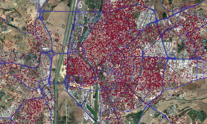
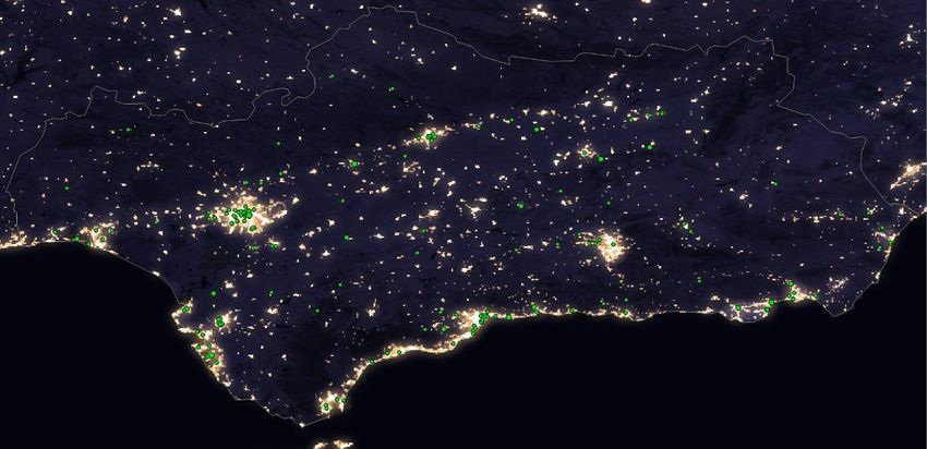
Lisbon, connecting the Island of Rhodes to the mainland, and one over the English
Channel to mimic the Channel Tunnel. All ferry lines have an assumed speed of 20 km/h,
and average fuel price for the EU at different distance-thresholds set to reflect ticket
prices as reported in Martino and Brambilla (2016), as explained below.
The size of the road network and the large number of routes to be calculated implies that
special care needs to be used to use a suitable and scalable method. We opted to use the
freeware osm2po tool10 to convert the OSM data into a PostgreSQL database residing on
a dedicated server with 40 cores and 240GB of RAM. This database was accessed using
the software R to start 40 parallel queries, each of them calculating a many-to-many
routing problem corresponding to an adequately sized portion of the origin-destination
matrix of centroids. The optimal routes themselves are calculated using the Dijkstra
algorithm from the pgRouting project.

3.2 Centroids
The centroids which are used to calculate driving time and transport costs originate from
a population density grid at a one square kilometer resolution, which was obtained from
the European Environmental Agency. Every square kilometer from the original raster is
populated with a randomly placed centroid for every 100 individuals estimated to inhabit
that area. Figure 1 below shows the centroids (the red dots) for the city of Seville,
superimposed on an aerial image from Google Earth, and the OSM road network used in
the analysis (in blue). The picture shows that the centroids are a quite good
approximation of the population density at a fine level of spatial disaggregation: there
are lots of dots in the historic centre (located within the curve of the old course of the
Guadalquivir river), but population density is higher in the newer (and cheaper)
residential areas to the north-east.

 Figure 1. The population grid for the urban area of Seville

Source: Own elaboration using Google Maps, OSM, and the European Environmental Agency population grid.

The full set of centroids generated from the population grid represents the location of
population quite precisely, even in excess of what is needed for our analysis. We
therefore do not consider all these centroids in the calculations, but rather take random
samples, with larger samples for region pairs at shorter distances. Table 1 shows the
sample sizes of centroids (dots) for each distance-threshold.

10
 See http://osm2po.de/

 6

Table 1. Centroid sample size used to calculate distances between regions
 Average
 Number of centroids
 Distance (d) Formula (area in km2) number of
 between
 centroids

 0 (intra-region) 250 and 120 min(250,max(area/100*3,120)) 229
 0 km

A population grid may underestimate the spatial concentration of the origin and
destination of freight flows, which may be dominated by a limited number of transport
hubs, industrial areas and sea-ports. The implicit assumption that freight flows are widely
spread in space which follows from sampling many points from a population grid is a
possible reason why we find relatively small effects of transport infrastructure investment
on the average trade costs between regions in section 5.

3.3 Data sources for the GTC
The GTC is composed by distance and time costs as per equation (1). To calculate each
component we assume all trips are made by a representative EURO VI truck (HDV)
consuming a constant rate of 34.5 L/100km (Dünnebeil et al., 2015).

3.3.1 Distance-related costs
The base fuel cost depends on fuel prices per member state (MS)12 and a constant rate of
fuel consumption. The fuel consumption is assumed to change with the slope of the road,
which we derive from the European digital elevation model for Europe developed by the
European Environment Agency.13 More concretely, an increase in the slope of a road
segment in absolute value of 1% increases fuel consumption by 5.5%, which corresponds
to the value of 11% found by Chen et al. (2017), adjusted for the fact that a positive
slope will be present only for either the trip or the return trip. This implies a fuel
consumption penalty of over 10% for about 15% of the roads with slopes in excess of
2%, and a penalty of over 44% for about 1% of the road segments which have a slope
higher than 8%.

Tolls are proportional to the distance travelled on toll roads. Van Essen et al. (2012)
provide detailed data for 2012 on the average toll-cost (in euros per km) for EU countries
based on road distance-related charges. Table 4 in Annex A reports the countries and the
tolls considered for the GTC.

For the tire ( ) and maintenance costs ( ) per km, we assume these costs to be
constant between all arcs in all MS. Specifically, they are set as to correspond to a joint
cost share of 9%, as found for Spain by Zofío et al. (2014).14

3.3.2 Time-related costs
The base travel time over an arc is calculated using the length of the arc and the
maximum allowed speed over the arc. This maximum speed is the value which is
provided for the segment in the OSM database. In case no value is provided in OSM, we
take the legal maximum speed for HDV in each MS and road type according to DG
MOVE.15 Nevertheless, further assumptions were taken to better reflect the real world
properties of the roads. These are the following:

 - The maximum speed on all primary roads was limited to the value from OSM or
 70 km/h, whichever was smaller. Likewise, the maximum speed on secondary
 roads was set to 60 km/h.
 - The presence of a traffic light adds 30 seconds to the travel time to cross the arc.
 - Curvature: the tortuosity of an arc is calculated as the ratio of the great circle
 distance between source and endpoint and the effective length of the road
 segment. We reduce the maximum speed by 2/3 for cases where the tortuosity of
12
 Fuel prices for each country are taken from “Europe’s Energy Portal” (https://energy.eu/).
13
 We use the raster map at a resolution of 1cmx1cm, which are interpolated values from the original 25mx25m
data. Available at: https://www.eea.europa.eu.
14
 Previous studies (Combes and Lafourcade, 2005; Zofío et al., 2014) find tire and maintenance costs to
represent a combined share in total cost of about 10% or less.
15
 Legal speed limits for HDV are taken from DG MOVE (European Commission). Available at:
http://ec.europa.eu/transport/road_safety/going_abroad

 8

the road exceeds 1.5, resulting in a speed of about 25 km/h on those segments
 on a primary road.
 - We divide the speed by 7 on surfaces like sand, cobblestone, etc. to give a typical
 speed of 10 km/h for a primary road with this surface type.
 - Roundabouts: we divide the maximum speed by 7 on roundabouts and highway
 ramps, to give a typical speed of 10 km/h on a on a roundabout on primary road.

All these changes affect the travel times which, jointly with salaries, are the main
determinants of the time costs. In our dataset, salaries include the definition of wages
and direct remuneration for the transport sector according to the European Labour Cost
Survey (2012) from Eurostat. Available information is at the NUTS 1 level for some
countries, while for most countries there are no regional data. We impute the same
salary for all the NUTS 2 regions contained within each NUTS 1 region with this
information, whereas in countries with no salaries at the regional level we use the
corresponding one at the national level for the transport sector.

Salaries are on an annual basis, so in order to compute a salary per minute to get a
measure equivalent in units with the travel time, we use the average hours worked per
week in each of the 28 EU MS published by Eurostat. Finally, we rely on European
Commission regulation ((EC) no. 561/2006) for resting times as an extra cost for travel
times. This regulation states that the driver must rest 45 min after 4 h driving and 11 h
after 9 h. In our case, resting times are considered as paid hours with the same salary
per hour as before, so we add resting times to the time economic cost as an additive
salary for those trips accomplishing the 2006 EC regulation.

3.3.3 Taxes and ferries costs of the GTC
Ownership taxes of HDV are paid yearly independently on the trade route the truck is
performing. However, it is reasonable to assume that the truck owner will transfer the
tax incidence to the client of the transport services – the firm shipping the goods.
Ownership taxes come from Van Essen, et al. (2012) and reported in Table 5 in Annex A.
Given the time needed to go from each origin to each destination, we compute the
number of trips that a truck can perform between each two regions within a year by
dividing the working hours in a year, including resting times, over the time needed to
travel the transport route via the cheapest route. Then, the ownership tax added to the
GTC of each trade link is calculated as the yearly ownership tax divided by the number of
trips that the truck can perform in a year.

Ferries are considered equivalent to a regular road route, with no gradients and
penalties. We follow Martino and Brambilla (2016) for the average price (cost) of a ferry-
ticket charged to passengers in the EU.16 This price varies according to three distance
thresholds: short (less than 100 km), medium (100-300 km) and large (more than 300
km). We add this cost of the ferry ticket per km as the fuel cost for ferries, depending on
the length (in km) of the ferry line. Table 6 in Annex A presents the different tickets (in
€/km) imputed for each ferry-arc.

3.3.4 Data sources for the iceberg trade costs
The iceberg trade cost matrix relies on trade flows among the EU regions. We resort to
Thissen et al. (2019) to get trade flows in monetary units and quantities (tonnes). These
authors estimate the inter-regional trade flows at NUTS 2 level for the EU using a set of
regionalized “Supply and Use” tables and probability matrices “derived from freight
transport data, airline data and business travel data, taking into account transhipments
locations (hub) and without pre-imposing any geographical structure on the data”. They

16
 This price concerns a trip with four persons and a car. The non-representative sample used by Martino and
Brambilla (2016) contains 50 observations. However, the values found by Martino and Brambilla closely match
the values which we found for ferry prices charged to a HDV.

 9

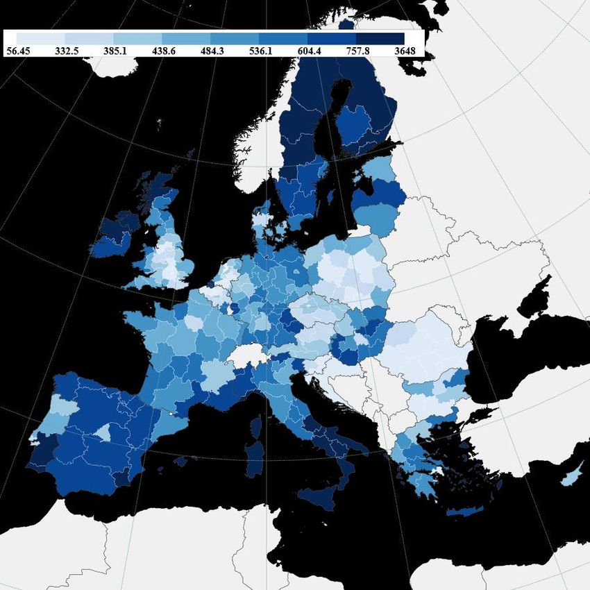
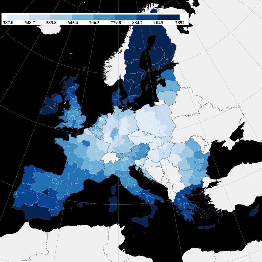
provide data for different sectors entailing goods and services in 2013. Given our GTC
approach based on transport costs by trucks, we take flow data in euros and tons for
manufacturing goods, agricultural and forestry products, and raw materials and energy
sources such as mining, quarrying, electricity and gas. 17

4. Descriptive analysis of the GTC
The full table with the estimated GTC between all pairs of 268 regions.18 This section
portraits a descriptive analysis of these estimates. Figure 3 plots the simple average GTC
across all destinies for each region , an inverse accessibility measure for each region. As
shown, geographically central regions have the lowest transport costs due to their
location within the road network, whereas far distant regions suffer from higher transport
costs.

 Figure 3. Average GTC for each NUTS 2 region

 Source: Own elaboration.

As described in section 2.1, the GTC is composed of many cost elements. As Table 2
portraits, fuel and time costs are the most predominant components, both representing
around 60% of the total transport cost. Time costs are mainly driven by salaries and, to
a lesser extent, by resting times. Distance costs in turn are determined by fuel prices and
fuel consumption. Ownership taxes represent a negligible share of costs, whereas the

17
 See Thissen et al. (2019) for a deeper understanding of the methodology behind the trade flows database.
18
 The GTC origin-destination matrix is available from the authors on request.

 10

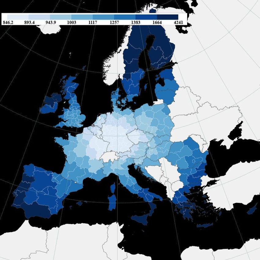
rest of the other costs (maintenance, accommodation, insurances, financing and
amortization costs, plus indirect costs) stand for the remaining 40% of the costs.

 Table 2. EU average GTC cost components

 Component Percentage

 Driver wage costs 42.1%

 Fuel costs 21.1%

 Ownership Taxes 0.6%

 Vignettes and Tolls 5.9%

 Other (time) 17.1%

 Other (distance) 13.3%

 Source: Own elaboration.

As can be observed in Table 3, the GTC has on average a value of 2,039€. The internal
GTC presents values of 2.42€ (for the city-region of Melilla measuring just 12km²) up to
759€ (for the Greek Southern Aegean region where the population is spread over 50
islands). The external GTC possesses more variability and highest average values.

 Table 3. EU GTC descriptive statistics

 GTC Observations Mean Std. Dev. Min Max

 Total 71,824 2,039.0 1,269.10 2.42 10,329.30

 Internal 268 101.3 78.00 2.42 758.73

 External 71,556 2,046.3 1,265.89 43.80 10,329.30

 Source: Own elaboration.

Distance and time costs are not only the most important components of the GTC, they
also show remarkable heterogeneity among regions. To reflect these regional differences,
Figure 4 separates out the (simple) average distance (a) and time (b) related costs of
each region. Distance costs are mainly driven by fuel consumption and fuel prices, so
regions that require shorter distances when travelling to other regions reduce
significantly their fuel consumption. That is why we see a core-periphery structure in
Figure 4a.

Salaries in the transport sector are the leading determinant of the time-related costs in
Figure 4b. Regions with lower salaries present lower GTC, while the opposite holds for
regions with high salaries. Far-distant regions require more time and resting times to
perform shipments by truck, forcing them to suffer higher GTCs even though salaries are
lower in these peripheral regions. This seems to be the cases of Greek, Portuguese,
Spanish, and southern Italian regions. Moreover, central regions in the road network also
benefit from low GTCs even in the eventual case of having high salaries in the transport
costs due to the lower required travel times. Western and central regions in Germany are
examples of this.

In summary, the GTC patterns reflect sources of comparative advantages across regions
caused either by their geographical location within the road network or by the time-
related costs. A core-periphery structure within the EU market emerges as a result of
regional differences in travel time and geographical distances.

 11

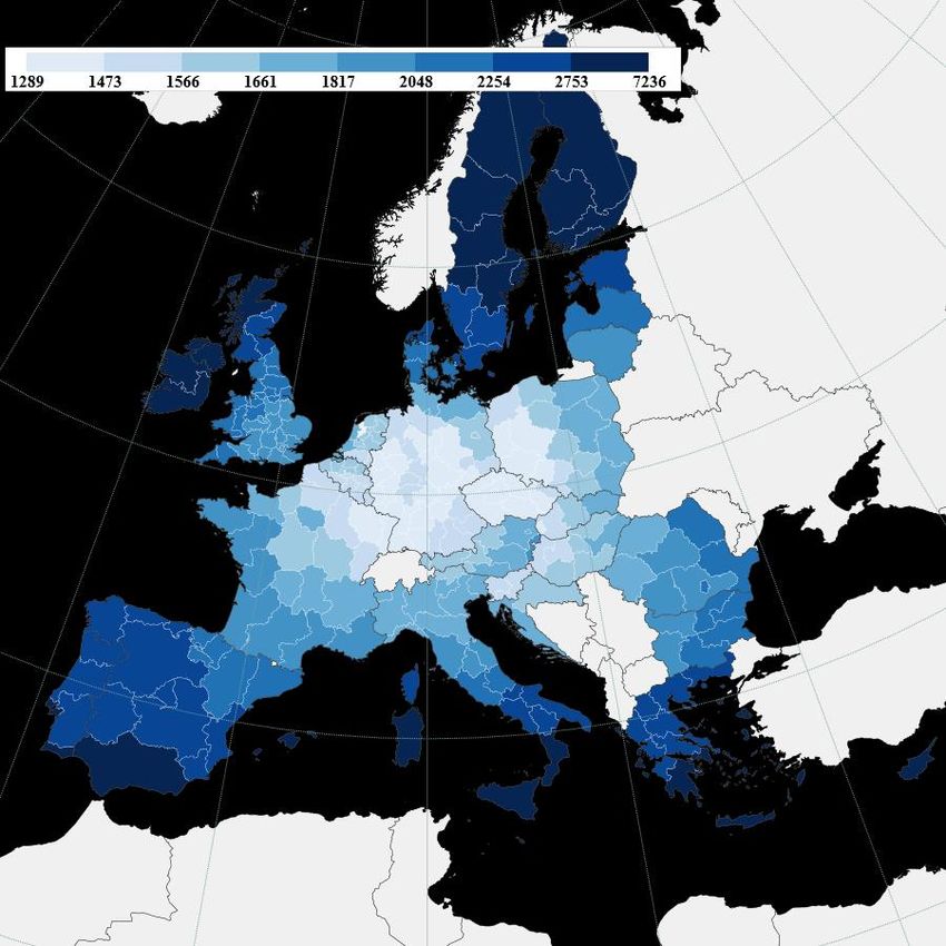
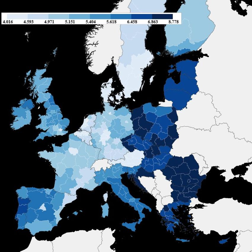
Figure 4. Distance and time related costs of GTC for each NUTS 2 region
 a) Distance-related costs

 Source: Own elaboration.

 b) Time-related costs

 Source: Own elaboration.

Alternatively, we consider the average GTC of each region weighing by the bilateral
trade flows between each pair using trade data from Thissen et al. (2019). This
weighted GTC more accurately reflects the average transport costs of a region in relation
to its trade partners. That is, the weighted version of the GTC captures both the trade
and transport costs links among regions. When graphically illustrating the effect of
policies on transport costs in a map, we will consider changes in this weighted version of

 12

the GTC as the most appropriate single index number summarising how the policy is
affecting individual regions. Figure 5 plots this weighted indicator. As shown, once trade
flows are included, truly integrated regions, as those in the core of Europe (regions in
Belgium, the Netherlands, or even the UK) are characterised by low transport costs. Most
of the Eastern European regions still benefit from low transport costs thanks to their low
time costs (salaries), although regions in Hungary do not present the same geographical
advantages as in Figure 3. Indeed the geographical pattern of trade will affect the
average trade costs: the fact that Greek regions now show a low average GTC reflects
the fact that the majority of their trade is over short distances, whereas far-located
regions highly dependent on long-distant trade still suffer from high transport costs. On
the contrary, the relatively high weighted average GTC German or Hungarian regions
may be due to trading over larger distances, or larger ratio of external relative to internal
trade flows.

 Figure 5. Average GTC weighted by trade flows for each NUTS 2 region

 Source: Own elaboration.

Up to now we focused on the spatial structure of the baseline GTC estimates. However,
an interesting application lies in the feasibility to perform policy experiments. By
modifying the components of the GTC, we can get an alternative transport cost matrix for
the EU regions. We compare this new counterfactual matrix with the baseline matrix to
get a new one with the (bilateral) changes in transport costs. As an example, in Figure 6
we plot the percentage change in the weighted GTC after a 20% increase in fuel prices
for all the regions. The darker regions are more affected by the increase in fuel prices as
fuel represents a relatively large share of their costs. These are regions where wages
(and therefore the share of labour costs) are lower, as well as their endowment of
infrastructure (see for instance the Eastern European regions), leading consequently to
higher fuel consumption.

 13

Figure 6. Change in the weighted GTC due to a 20% increase in fuel prices

 Source: Own elaboration.

5. Policy simulations: Transport infrastructure investment
In order to estimate the effect of transport infrastructure investment on transport costs,
we identify those roads that would create the largest net economic benefit when being
upgraded to a highway. For the cost of upgrading, we take the estimated cost of building
a km of highways in the EU from the European Court of Auditors (2013). We adjusted
this construction cost per country by applying the Eurostat price level index for civil
engineering construction projects. In Annex A, Tables 7 and 8 respectively show the
baseline cost for building highways and the adjustments per country. This cost is further
adjusted depending on several road properties: we increase the cost by 10% for every
1% increase in the slope of the road; by 30% for every 1000 inhabitants in a 1 km radius
around the road; by 70% if the road is a bridge or tunnel.

We identify roads for upgrading by comparing the economic cost of upgrading to the
economic benefit. To calculate the benefit, we look for network segments which are the
most important bottlenecks for traffic. This is done by ranking the primary and secondary
roads in each region according to the estimated traffic (in number of trucks) over them,
per lane.19 The traffic between two centroids and belonging to regions and 
respectively, is assumed to depend on the flow of goods in tonnes between the regions
 and ; the estimated number of trucks required to perform the transport of 1 tonne of
goods, ; the great-circle distance dist between the centroids and ; and finally, the
population share of both the centroid of origin and destination in the respective regional
populations. More specifically, we assume that the number of trucks travelling between
centroids and equals the following:

19
 This approach obviously does not mean to suggest that the improved roads are always a choice policy makes
will or should make, and oftentimes it is not realistic to assume that a specific road segment would be
improved. Nevertheless, we believe the approach can provide an estimate of how the transport costs would
change in case of real world, fully planned road infrastructure projects.

 14

( + ) 1
 = (7)
 2 

The effect of transport infrastructure investment will depend on the number of centroids,
that is, when using more centroids, traffic will be spread over more roads, and
improvements in a road segment will affect a proportionally smaller share of transport.
However, given that (especially in cities) centroids may be sampled at arbitrarily close
distances, these would be assigned overly large shares of the trade flows. We therefore
impose a minimum distance of 15km.

Primary and secondary roads then are ranked according to the difference between the
aggregate generalised transport cost, calculated by multiplying the GTC of the arc by the
number of trucks travelling over them, compared to the aggregate cost assuming the arc
is upgraded. We then progress by changing the characteristics of the primary and
secondary roads earmarked for upgrading to match those of a motorway: removing any
speed or distance penalty due to the presence of traffic lights, roundabouts, surface
material, curvature or slope, and increasing the effective speed to 90 km/h. The road
segments are changed sequentially starting from the arc with the largest estimated net
economic gain from upgrading, up to the point where a segment improvement can no
longer be financed for more than 50% (this ensures that on average all the investment
money is spent, although individual regions will have some small amount of over- or
underspending). We exclude toll costs from being affected by policies, as it is unclear
whether or how constructing a highway would change toll costs on a given route.

Figure 7 below shows the change in transport costs when all the EU regions receive the
same amount of investment (€500 million). Centrally-located regions benefit the most as
a result of the spillover effects among regions. That is, although all the EU regions
experience a reduction in transport costs, those that are located in the core of the road
network enjoy the highest benefits in terms of spillover from neighbouring regions
(Condeço-Melhorado et al., 2011). An important determinant of the observed change in
transport cost is the size of the region: we observe larger effects in the smaller regions
in, Belgium, the Netherlands, and Germany compared to the larger regions in Spain and
France.

 15

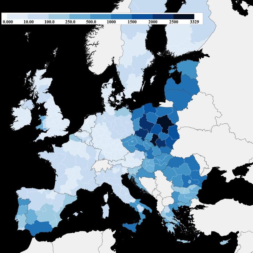
Figure 7. Change in weighted GTC as a result of investing 500M€ in each NUTS 2 region

 Source: Own elaboration.

Next, we turn to the EU’s 2014-2020 Cohesion Policy programme. Figure 8 shows the
total amounts invested per region, adding up investments in all types of transport
infrastructure and considering expenditure over the entire programming period. The
programme clearly targets regions in Poland, Romania, Slovakia, and the Baltic
countries. There are smaller investments in Southern Italy and Spain.

 16

Figure 8. Transport Infrastructure investment in the Cohesion Programme 2014-2020 (Millions of €)

 Source: Own elaboration.

Figure 9 portraits the simulated change in transport costs due to the transport
infrastructure investment. Given that the EU Cohesion Policy is a targeted policy for less
endowed regions, Eastern European regions are, overall, the ones with the highest
reduction in transport costs. However, there are significant spillovers to non-targetted
regions, such as some Eastern and Central German and Northern Italian regions. There is
much less impact on some targeted regions in the south of Spain.

We then separately consider changes in transport costs within the region (Panel b) and
between regions (Panel c). As for the former, the regions with a less developed road
network like in Eastern Europe show the largest reduction in internal transport costs.

Complementary to this, transport costs between regions (Panel c) follow the same
pattern as the overall transport costs. This panel shows some clear evidence of spillover
effects in Eastern Germany and Northern Italy, which benefit from a reduction in their
external transport cost even without receiving many funds directly. Understandably
because of its location, also Southern Finland emerges as a region which benefits
significantly from the large investments in road infrastructure in the Baltic countries and
Central and Eastern Europe.

 17

Figure 9. Change in the GTC due to the Cohesion Policy investment
 a) Percentage change in the weighted GTC

 b) Percentage change in the internal GTC

 18

c) Percentage change in the external weighted GTC

 Source: Own elaboration.

6. Conclusion
Transport costs are not usually well captured in spatial economic models. In an attempt
to overcome this limitation, we create a unique dataset of interregional transport costs
for the EU regions (NUTS 2) by taking use of the open digitalised road network OSM.
Combining this database with other information allows us to calculate the optimal route
of transport by truck and calculate the associated average transport cost between
regions. A first contribution of our paper is to provide a comprehensive set of transport
cost estimates between EU regions at the NUTS2 level, along with a set of underlying
variable such as driving times and distances.

The results indicate that transport costs follow a core-periphery structure within the EU,
where geographically central regions benefit from shorter trips and reduced fuel
consumption, and more peripheral regions tend to benefit from lower salaries within the
transport sector.

Moreover, the method allows performing transport policy analysis. We provide an
example in this paper by studying the effects of a generalised increase in fuel prices. We
describe a tool for policy analysis on transport infrastructure investment. We apply it to
estimate the impact of the EU’s 2014-2020 Cohesion Policy programme, showing that
Eastern European regions are the regions benefitting the most from road infrastructure
investments, with positive spillover effects across the whole EU, but especially to
neighbouring regions.

In future research, we aim to expand the definition of transport costs considered to
include also costs related to loading/unloading or warehousing, and to consider other
modes such as rail or inland waterways. Clearly, including more costs would reduce the

 19

estimated impact of any infrastructure investment on such a wider definition of trade and
transport costs. This would be especially the case for transport costs internal to the
region or neighbouring regions, where these additional costs may be expected to
represent a larger share of the total trade and transport cost. Other aspects of the
analysis that can be improved are the use information on land-use to better estimate the
origin and destination of the freight flows, which are now assumed to be distributed
according to the population grid; and to use more information on the specifics of goods
and sectors such as loading factors or volume/weight ratio's.

7. References
Chen, Y., Zhu, L., Gonder, J., Young, S., and Walkowicz, K. (2017). Data-driven fuel
consumption estimation: A multivariate adaptive regression spline approach.
Transportation Research Part C: Emerging Technologies 83, 134-145.

Combes, P.P. and Lafourcade, M. (2005). Transport Costs: Measures, Determinants, and
Regional Policy Implications for France. Journal of Economic Geography 5 (3), 319–49.

Condeço-Melhorado, A., Martín, J. C., and Gutiérrez, J. (2011). Regional spillovers of
transport infrastructure investment: A territorial cohesion analysis. EJTIR 4(11), 389-
404.

Dijkstra, E.W. (1959). A note on two problems in connexion with graphs. Numerische
Mathematik 1(1), 269-271.

Dünnebeil, F., Reinhard, C., Lambrecht, U., Kies, A., Hausberger, S., and Rexeis, M.
(2015). Future measures for fuel savings and GHG emission reduction of heavy-duty
vehicles. Federal Environment Agency, Germany, TEXTE 32/2015.

European Court of Auditors (2013). Are EU cohesion policy funds well spent on roads?.
European Court of Auditors, Special Report No. 5, Luxembourg, ISBN 978-92-9241-270-
8.

Eurostat (2016). Road Freight Transport Methodology. Eurostat, Luxembourg, ISBN 978-
92-79-60068-5.

Head, K., and Mayer, T. (2009) Illusory border effects: distance mismeasurement inflates
estimates of home bias in trade. In: The Gravity Model in International Trade: Advances
and Applications. Editors: Bergeijk and Brakman.

Hillberry, R. and Hummels, D. (2013). Trade elasticity parameters for a computable
general equilibrium model. Handbook of computable general equilibrium modelling,
Elsevier, Vol. 1, 1213-1269.

Hummels, D. (1999). Toward a geography of trade costs. GTAP Working Paper No. 17.

Jacobs-Crisioni, C., Silva, F.B., Lavalle, C., Baranzelli, C., Barbosa, A., and Castillo, C.P.
(2016). Accessibility and territorial cohesion in a case of transport infrastructure
improvements with changing population distributions. European Transport Research
Review 8(1), 9.

Lecca, P., Barbero, J., Christensen, M., Conte, A., Di Comite, F., Diaz-Lanchas, J.,
Diukanova, O., Mandras, G., Persyn, D., and Sakkas, S. (2018). RHOMOLO V3: A Spatial
Modelling Framework. EUR 29229 EN, Publications Office of the European Union,
Luxembourg, 2018, ISBN 978-92-79-85886-4.

 20

Martino, A. and Brambilla, M. (2016). Research for TRAN Committee-The EU Maritime
Transport System: Focus on Ferries, European Parliament, Committee on Transport and
Tourism, Brussels.

Martinez-Zarzoso, I. and Nowak-Lehmann, F.D. (2007). Is distance a good proxy for
transport costs? The case of competing transport modes. The Journal of International
Trade & Economic Development 16(3), 411-434.

Teixeira, A. C. (2006). Transport policies in light of the new economic geography: The
Portuguese experience. Regional Science and Urban Economics 36(4), 450-466.

Thissen, M., Husby, T. Ivanova, O., and Mandras, G. (2019). European NUTS 2 regions:
construction of interregional trade-linked Supply and Use tables with consistent transport
flows. JRC Working Papers on Territorial Modelling and Analysis No. 01/2019, European
Commission, Seville, 2019, JRC115439.

Van Essen, H., Nelissen, D., Smit, M., Van Grinsven, A., Aarnink, S., Breemersch, T.,
Martino, A., Rosa, C., Parolin, R., and Harmsen, J. (2012). An inventory of measures for
internalising external costs in transport. European Commission, Directorate-General for
Mobility and Transport, Brussels, DM 28 – 0/110.

Zofío, J. L., Condeço-Melhorado, A. M., Maroto-Sánchez, A., and Gutiérrez, J. (2014).
Generalized transport costs and index numbers: A geographical analysis of economic and
infrastructure fundamentals. Transportation Research Part A: Policy and Practice 67, 141-
157.

 21

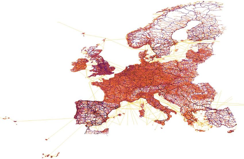
Annex A: Data description and further figures

A.1 The Road Network
The subset of the OSM road network used in the analysis contains motorways, trunk
roads, primary roads, secondary roads and ferry lines, for a total length of about
1.500.000 km over a surface area of about 5.730.000 km², giving an average road
density of 0.26 km/km².

 Figure 10. Road and ferries networks (2017)

Source: OSM.

A.2 Tolls
 Table 4. Tolls considered in each country for Heavy Duty Vehicles (2018)
 Country Cost per km Toll applied on Yearly Source
 (EUR) vignette
 (EUR)
 Austria 0.419 Highway and asfinag.at
 Schnellbahn go-maut.at
 Belgium 0.142 All highways viapass.be
 and selected
 national roads
 Bulgaria 1066 web.bgtoll.bg
 Croatia 0.18 All highways Sample route on hac.hr
 (Zagreg-Dubrovnik)
 Czech Republic 0.18 OSM toll tag mytocz.eu
 Denmark 1250 EUR Eurovignettes.eu
 Estonia 1100 Teetasu.ee
 France 0.24 all highways Sample routes on
 autoroutes.fr
 (Marseille-Paris and
 Aix-en-Provence to
 Lyon)
 Germany 0.198 All highways Toll-collect.de
 and primary

 22

roads
 Greece 0.197 All highways Sample route on
 diodia.com.gr (Athens-
 Patras)
 Hungary 0.32 highway OSM toll tag hu-go.hu
 0.2 primary
 Latvia 711 Lvvignette.eu
 Lithuania 753 Keliumokestis.lt
 Luxembourg 1250 Eurovignettes.eu
 Ireland 0.063 All highways Sample route on
 www.tii.ie (Galway-
 Dublin)
 Italy 0.18 All highways Sample route on
 autostrade.it (Milan-
 Bari)
 Netherlands 1250 Eurovignettes.eu
 Poland 0.27 All highways Viatoll.pl
 Portugal 0.18 All highways Sample route on
 estradas.pt (Porto-
 Lisbon)
 Romania 1210 Roviniete.ro
 Slovakia 0.19 highway All highway and Emyto.sk
 0.16 primary primary roads
 Slovenia 0.38 All highways dars.si
 Spain 0.286 OSM tag Van Essen et al. (2012)
 Sweden 1250 Eurovignettes.eu
United Kingdom 740 Multiservicetolls.com
 Norway 0.068 All highways Sample route on
 fjellinjen.no
 (Fredrikstad –
 Kristiansand)
 Switzerland 0.81 All highways Ezv.admin.ch

A.3 Taxes
 Table 5. Ownership Taxes by country (EU, 2012)
 Country Tax (in euros)
 Belgium 517€
 Bulgaria 1833.63€
 Czech Republic 1772.63€
 Denmark 517.85€
 Germany 556€
 Estonia 515.2€
 Ireland 3160€
 Greece 1320€
 Spain 392.74€
 France 516€
 Croatia N/A (set at 0)
 Italy 549.92€
 Cyprus 521€
 Latvia 507.61€
 Lithuania 654.54€
 Luxembourg 520€
 Hungary 1503.57€

 23

Malta 515€
 Netherlands 876€
 Austria 912€
 Poland 801.32€
 Portugal 713€
 Romania 510.92€
 Slovenia 2347.25€
 Slovakia 1033.74€
 Finland 1460€
 Sweden 3675.54€
 United Kingdom 1570.5€
 Source: Van Essen et al. (2012).

A.4 Ferry ticket prices
 Table 6. Ferry ticket prices per kilometre (EU, 2015)
 Range Distance (in Average price
 km) (€/km)
 Short Less than 100 2.74
 Medium 100-300 1.73
 Long More than 300 1.06
 Source: Martino and Brambilla (2016).

A.5 Infrastructure costs
 Table 7. Average cost per kilometre of different type of roads (EU, 2013)
 Type of road Average cost (€/km)
 Highway 10,941,402
 Primary Roads 6,225,187
 Secondary Roads 4,159,281
 Source: Eurpean Court of Auditors (2013).

 Table 8. Civil engineering works price level index (2016, EU27=100)
 Country 2016
 Belgium 103.4
 Bulgaria 67.4
 Czech
 Republic 82.4
 Denmark 139.0
 Germany 130.3
 Estonia 88.3
 Ireland 92.9
 Greece 73.1
 Spain 77.0
 France 134.3
 Croatia 66.9
 Italy 82.6
 Cyprus 83.6
 Latvia 71.8
 Lithuania 84.8
 Luxembourg 119.8

 24

Hungary 65.4
Malta 105.2
Netherlands 108.3
Austria 112.6
Poland 87.3
Portugal 57.9
Romania 52.6
Slovenia 89.0
Slovakia 79.0
Finland 157.2
Sweden 146.7
United Kingdom 115.2
Source: Eurostat.

 25

GETTING IN TOUCH WITH THE EU
In person
All over the European Union there are hundreds of Europe Direct information centres. You can find the
address of the centre nearest you at: https://europa.eu/european-union/contact_en
On the phone or by email
Europe Direct is a service that answers your questions about the European Union. You can contact this
service:
- by freephone: 00 800 6 7 8 9 10 11 (certain operators may charge for these calls),
- at the following standard number: +32 22999696, or
- by electronic mail via: https://europa.eu/european-union/contact_en
FINDING INFORMATION ABOUT THE EU
Online
Information about the European Union in all the official languages of the EU is available on the Europa
website at: https://europa.eu/european-union/index_en
EU publications
You can download or order free and priced EU publications from EU Bookshop at:
https://publications.europa.eu/en/publications. Multiple copies of free publications may be obtained by
contacting Europe Direct or your local information centre (see https://europa.eu/european-
union/contact_en).