Estimation of the Antarctic surface mass balance using the regional climate model MAR (1979-2015) and identification of dominant processes
←
→
Page content transcription
If your browser does not render page correctly, please read the page content below
The Cryosphere, 13, 281–296, 2019
https://doi.org/10.5194/tc-13-281-2019
© Author(s) 2019. This work is distributed under
the Creative Commons Attribution 4.0 License.

Estimation of the Antarctic surface mass balance using the regional
climate model MAR (1979–2015) and identification
of dominant processes
Cécile Agosta1,2,3 , Charles Amory1 , Christoph Kittel1 , Anais Orsi2 , Vincent Favier3 , Hubert Gallée3 ,
Michiel R. van den Broeke4 , Jan T. M. Lenaerts4,5 , Jan Melchior van Wessem4 , Willem Jan van de Berg4 , and
Xavier Fettweis1
1 F.R.S.-FNRS,    Laboratory of Climatology, Department of Geography, University of Liège, 4000 Liège, Belgium
2 Laboratoire   des Sciences du Climat et de l’Environnement (IPSL/CEA-CNRS-UVSQ UMR8212), CEA Saclay,
91190 Gif-sur-Yvette, France
3 Université Grenoble Alpes, CNRS, Institut des Géosciences de l’Environnement, 38000, Grenoble, France
4 Institute for Marine and Atmospheric Research Utrecht, Utrecht University, Utrecht, the Netherlands
5 Department of Atmospheric and Oceanic Sciences, University of Colorado Boulder, Boulder, CO, USA

Correspondence: Cécile Agosta (cecile.agosta@gmail.com)

Received: 12 April 2018 – Discussion started: 20 April 2018
Revised: 27 December 2018 – Accepted: 3 January 2019 – Published: 29 January 2019

Abstract. The Antarctic ice sheet mass balance is a major          vious model-based estimates and need to be better resolved
component of the sea level budget and results from the dif-        and constrained in climate models. Sublimation of precipi-
ference of two fluxes of a similar magnitude: ice flow dis-        tating particles in low-level atmospheric layers is responsi-
charging in the ocean and net snow accumulation on the ice         ble for the significantly lower snowfall rates in MAR than in
sheet surface, i.e. the surface mass balance (SMB). Sepa-          RACMO2 in katabatic channels at the ice sheet margins. At-
rately modelling ice dynamics and SMB is the only way to           mospheric sublimation in MAR represents 363 Gt yr−1 over
project future trends. In addition, mass balance studies fre-      the grounded ice sheet for the year 2015, which is 16 % of
quently use regional climate models (RCMs) outputs as an           the simulated snowfall loaded at the ground. This estimate
alternative to observed fields because SMB observations are        is consistent with a recent study based on precipitation radar
particularly scarce on the ice sheet. Here we evaluate new         observations and is more than twice as much as simulated in
simulations of the polar RCM MAR forced by three reanal-           RACMO2 because of different time residence of precipitat-
yses, ERA-Interim, JRA-55, and MERRA-2, for the period             ing particles in the atmosphere. The remaining spatial differ-
1979–2015, and we compare MAR results to the last outputs          ences in snowfall between MAR and RACMO2 are attributed
of the RCM RACMO2 forced by ERA-Interim. We show                   to differences in advection of precipitation with snowfall par-
that MAR and RACMO2 perform similarly well in simu-                ticles being likely advected too far inland in MAR.
lating coast-to-plateau SMB gradients, and we find no sig-
nificant differences in their simulated SMB when integrated
over the ice sheet or its major basins. More importantly, we
outline and quantify missing or underestimated processes in        1   Introduction
both RCMs. Along stake transects, we show that both models
accumulate too much snow on crests, and not enough snow            Mass loss from the Antarctic ice sheet (AIS) and therewith
in valleys, as a result of drifting snow transport fluxes not      its contribution to the sea level budget results from the differ-
included in MAR and probably underestimated in RACMO2              ence of two fluxes of a similar magnitude: ice flow discharg-
by a factor of 3. Our results tend to confirm that drifting snow   ing in the ocean (D) and net snow accumulation on the ice
transport and sublimation fluxes are much larger than pre-         sheet surface, i.e. the surface mass balance (SMB). The total

Published by Copernicus Publications on behalf of the European Geosciences Union.
282                                                                                C. Agosta et al.: Antarctic SMB using MAR

ice sheet mass balance (SMB minus D) can be assessed using          mon biases against observed SMB, resulting from drifting
satellite altimetry, gravimetry, or the input–output method         snow transport fluxes. Secondly, we analyse SMB differ-
(Shepherd et al., 2018), which all request SMB estimates.           ences among models and show that many of the discrepan-
The input–output method, which consists in separately mod-          cies can be attributed to low-level sublimation of precipita-
elling ice dynamics and SMB, is also the only way to project        tion in katabatic channels and to the difference in precipita-
future trends.                                                      tion advection inland. Finally, in Sect. 4, we summarise our
   SMB as used in this study is the sum of mass gains               main findings and discuss further efforts to be achieved for a
(mainly snowfall accumulation and some riming), mass                better assessment of the AIS SMB.
losses (mainly surface and drifting snow sublimation, some
liquid water run-off), and drifting snow transport (defined as
the horizontal advection of the drifting snow), which can lead      2     Data and methods
to either mass gain or mass loss. Snowfall rates are 1 order
of magnitude larger than all of the other SMB fluxes at the         2.1     Regional modelling
continental scale (Lenaerts et al., 2012b), with the largest
amounts found along the ice sheet margins due to cyclonic           2.1.1    Regional atmospheric models
activity in the Southern Ocean and to the orographic lifting
of relatively warm and moist air masses (van Wessem et al.,         For the first time, the polar-oriented regional atmospheric
2014; Favier et al., 2017). Accumulation patterns are highly        model MAR is applied for decades-long simulations over the
variable at the kilometre scale and from year to year (e.g.         whole AIS. MAR atmospheric dynamics are based on the
Agosta et al., 2012). Consequently, proper observations of          hydrostatic approximation of the primitive equations, fully
SMB require a high spatial coverage (e.g. stake lines, accu-        described in Gallée and Schayes (1994). Prognostic equa-
mulation radars plus ice cores for layer dating and snow den-       tions are used to depict five water species: specific humid-
sity) and a temporal sampling spanning several years (Eisen         ity, cloud droplets and ice crystals, raindrops, and snow par-
et al., 2008). Even if efforts have been made to fulfil those re-   ticles (Gallée, 1995). Sublimation of airborne snow parti-
quirements, ground-based observations are scarce and carry          cles is a direct contribution to the heat and moisture bud-
with them high logistical costs in this cold, windy, and re-        get of the atmospheric layer in which these particles are
mote environment. Interpolation techniques used to inter-           simulated. The radiative transfer through the atmosphere is
polate the scarce SMB observations (Vaughan et al., 1999;           parametrised as in Morcrette (2002), with snow particles af-
Arthern et al., 2006) encounter major caveats (Magand et al.,       fecting the atmospheric optical depth (Gallée and Gorodet-
2008; Genthon et al., 2009; Picard et al., 2009).                   skaya, 2010). The atmospheric component is coupled to the
   This is why many AIS mass balance studies use output of          surface scheme SISVAT (soil ice snow vegetation atmo-
regional climate models (RCMs) to estimate ice sheet SMB            sphere transfer; De Ridder and Gallée, 1998) dealing with
for the recent decades (e.g. Rignot et al., 2011; Gardner et al.,   the energy and mass exchanges among surface, snow, and at-
2018; Shepherd et al., 2018). In order to obtain a good agree-      mosphere. The snow-ice part of SISVAT is based on the snow
ment with observations, atmospheric models require accurate         model CROCUS (Brun et al., 1992). It is a one-dimensional
large-scale circulation patterns together with a proper rep-        multilayered energy balance model which simulates meltwa-
resentation of snow surface processes, clouds, and turbulent        ter refreezing, snow metamorphism, and snow surface albedo
fluxes and a relatively high horizontal resolution to properly      depending on snow properties. We used MAR version 3.6.4,
resolve the complex ice sheet topography at the margins.            simply called MAR hereafter. In this version the physical set-
   Here, we present new simulations of the RCM MAR,                 tings are the same as in MAR version 3.5.2 used for Green-
applied for the first time over the whole AIS, but already          land (Fettweis et al., 2017), except for the adaptations de-
widely used for polar studies, e.g. in Greenland (Fettweis          tailed below.
et al., 2013, 2017), Svalbard (Lang et al., 2015), Adélie Land         Grid. Projection is the standard Antarctic polar stereo-
(Antarctic coastal area; Gallée et al., 2013; Amory et al.,         graphic method (EPSG:3031). The horizontal resolution is
2015), and Dome C (Antarctic plateau; Gallée et al., 2015).         35 km, an intermediate resolution that results from a com-
We compare MAR-simulated SMB with the state-of-the-art              putation time compromise in order to run the model with
RCM RACMO2 (van Wessem et al., 2018). We use avail-                 multiple reanalyses and global climate model forcings over
able SMB observational datasets to show that MAR and                the 20th and the 21st centuries. The vertical discretisation
RACMO2 perform similarly well in simulating the SMB spa-            is composed of 23 hybrid levels from ∼ 2 m to ∼ 17 000 m
tial gradients. In addition, we identify significant processes      above the ground.
that still need to be included or improved in both RCMs.               Boundaries. The topography is derived from the Bedmap2
   In Sect. 2, we describe MAR and its specific set-up for          surface elevation dataset (Fretwell et al., 2013). Because the
Antarctica, together with RACMO2, the forcing fields, ob-           Antarctic domain is about 4 times larger than the Green-
servational datasets, and methods designed for model eval-          land domain, the circulation has to be more strongly con-
uation. In Sect. 3, we show that both RCMs share com-               strained. This is why we use a boundary relaxation of temper-

The Cryosphere, 13, 281–296, 2019                                                        www.the-cryosphere.net/13/281/2019/

C. Agosta et al.: Antarctic SMB using MAR 283
ature and wind in the upper atmosphere starting from 400 hPa 2.1.2 Forcing reanalyses
(∼ 6000 m above the ground) to 50 hPa (upper level), as in
van de Berg and Medley (2016), whereas relaxation starts Regional atmospheric models are forced by atmospheric
from 200 hPa in Fettweis et al. (2017). fields at their lateral boundaries (pressure, wind, temper-
Parameterisations. ature, humidity), at the top of the troposphere (tempera-
ture, wind), as well as by sea surface conditions (sea ice
a. The surface snow density ρs (kg m−3 ) is computed as a concentration, sea surface temperature) every 6 h. Conse-
function of 10 m wind speed ws10 (m s−1 ) and surface quently, regional atmospheric models add details and physics
temperature Ts (K): to the forcing model in the middle and lower troposphere
and at the land or iced surface, whereas large-scale circu-
ρs = 149.2 + 6.84 ws10 + 0.48 Ts , (1) lation patterns are driven by the forcing fields. We forced
MAR with three reanalyses over Antarctica in order to eval-
with minimum–maximum values of 200–400 kg m−3 . uate the uncertainty in the simulated surface climate arising
This parameterisation was defined so that the simulated from the uncertainty in the assimilation systems: the Euro-
density of the first 50 cm of snow fits observations col- pean Centre for Medium-Range Weather Forecasts “Interim”
lected over the AIS (see Fig. S1, with the snow density re-analysis (hereafter ERA-Interim, resolution ∼ 0.75◦ , i.e.
database detailed in Table S1 in the Supplement). ∼ 50 km at 70◦ S; Dee et al., 2011), the Modern-Era Retro-
spective Analysis for Research and Applications version 2
(hereafter MERRA-2, resolution ∼ 0.5◦ ; Gelaro et al., 2017),
b. The aerodynamic roughness length z0 is computed as a and the Japanese 55-year Reanalysis from the Japan Me-
function of the air temperature, as proposed in Amory teorological Agency (hereafter JRA-55, resolution ∼ 1.25◦ ;
et al. (2017). The parameterisation was tuned so that Kobayashi et al., 2015).
z0 fit the observed seasonal variation between high The regional atmospheric model RACMO2 is forced by
(> 1 mm) summer and lower (0.1 mm) winter values in ERA-Interim. We focus our study to the period 1979–2015,
coastal Adélie Land, for air temperatures above −20 ◦ C. as reanalyses are known to be unreliable before 1979, when
For lower temperatures, z0 is kept constant and set to satellite sounding data started to be assimilated (Bromwich
0.2 mm, in agreement with observed z0 values on the et al., 2007).
Antarctic plateau (e.g. Vignon et al., 2016);
2.2 Observations
c. As in Fettweis et al. (2017), the MAR drifting snow
scheme is not activated because this scheme was sen- 2.2.1 SMB observations and sectors of strong SMB
sitive to parameter choices (Amory et al., 2015). An up- gradients
dated version of the drifting snow scheme is currently
being developed and evaluated for application at the We use SMB observations of the GLACIOCLIM-SAMBA
scale of the whole ice sheet. dataset detailed in Favier et al. (2013) and updated by
Wang et al. (2016). This dataset is an update of the one
We compare MAR results over the AIS to the latest out- assembled by Vaughan et al. (1999) following the quality-
puts of the regional atmospheric model RACMO2 version control methodology defined by Magand et al. (2007). It in-
2.3p2 (van Wessem et al., 2018), called RACMO2 hereafter, cludes 3043 reliable SMB values averaged over more than
using a horizontal resolution of 27 km, a vertical resolution 3 years. We add accumulation estimates from Medley et al.
of 40 atmospheric levels, and a topography based on the dig- (2014), retrieved over the Amundsen Sea coast (Marie Byrd
ital elevation model from Bamber et al. (2009). This regional Land) with an airborne-radar method combined with ice-core
model is developed by the Royal Netherlands Meteorologi- glaciochemical analysis.
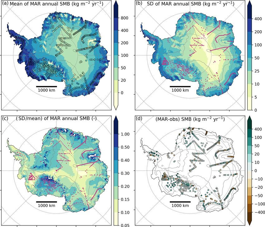
cal Institute (KNMI) and has subsequently been adapted for The first-order feature of the Antarctic SMB is a strong
modelling the Antarctic climate and its SMB (van de Berg coastal–inland gradient, with mean values ranging from typi-
et al., 2006). It includes a drifting snow scheme (Lenaerts cally greater than 500 kg m−2 yr−1 at the ice sheet margins to
et al., 2012a), an albedo routine with prognostic snow grain about 30 kg m−2 yr−1 in the dry interior plateau (Fig. 1a; see
size (Kuipers Munneke et al., 2011), and a multilayer snow also, e.g. Wang et al., 2016). As observations only cover 5 %
model computing melt, percolation, refreezing, and run-off of MAR grid cells over the ice sheet, we divide that sparse
(Ettema et al., 2010). observation dataset into 10 sectors detailed in Table 1 and
MAR and RACMO2 models were developed indepen- shown in Fig. 2. Six of them are stake transects with a stake
dently. We will not detail here the many physical parame- every ∼ 1.5 km, which have been proven very valuable for
terisation differences between both RCMs, but we will later evaluating modelled SMB (Agosta et al., 2012; Favier et al.,
highlight some of them we show having a significant impact 2013; Wang et al., 2016). The four other sectors are com-
on the modelled SMB. posed of more scattered observations covering large eleva-
www.the-cryosphere.net/13/281/2019/ The Cryosphere, 13, 281–296, 2019
284 C. Agosta et al.: Antarctic SMB using MAR
tion ranges (Victoria Land, Dronning Maud Land, and Ross of −3 kg m−2 yr−1 , R 2 = 0.86, computed on the logarithm
Ice Shelf–Marie Byrd Land). of SMB as well).
The model–observation comparison by sectors (Fig. 2)
2.2.2 Model–observation comparison method reveals a good representation of the coast-to-plateau SMB
gradients by both RCMs. MAR and RACMO2 are in good
RACMO2 outputs are bilinearly interpolated to the 35 × agreement despite MAR not including drifting snow pro-
35 km MAR grid. For each SMB observation, we con- cesses whereas RACMO2 does, except in Ross–Marie Byrd
sider the four surrounding MAR grid cells, from which we Land and in Victoria Land where MAR simulates larger
eliminate ocean grid cells. We also eliminate surrounding SMB than RACMO2. Another noticeable result is that MAR
grid cells with an elevation difference with the observation forced by ERA-Interim, JRA-55, and MERRA-2 gives very
greater than 200 m (missing elevation of observation is set similar results for the SMB spatial pattern, not only at the
to Bedmap2 elevation at 1 km resolution). Finally, we bilin- observation locations (Fig. 2) but also at the ice sheet scale
early interpolate model values of the remaining grid cells at (comparisons of MAR SMB for different forcing reanalyses
the observation location (see schematic in Fig. S2). are shown in Fig. S4, with colour map scales 10 times smaller
As we restrict our modelling study to the 1979–2015 pe- than in Fig. S5 in which MAR is compared to RACMO2).
riod, we only consider observations beginning after 1950. For This is why we focus on MAR forced by ERA-Interim in the
observations beginning after 1979, we time-average model following.
outputs for the same period as the observation. We keep ob- We find no significant differences in the SMB simulated by
servations beginning before 1979 only if they cover more MAR and RACMO2 when integrated over the ice sheet or its
than 8 years, and in this case we compare the observed value major basins (Table 2). SMB is driven by snowfall amounts,
with the modelled value time-averaged for 1979–2015. which are more than 10 times larger than other SMB compo-
In a last step, we average-out the kilometre-scale variabil- nents. Snow sublimation in RACMO2 is the sum of sublima-
ity in the observed SMB (Agosta et al., 2012) by binning tion at the surface of the snowpack and of drifting snow subli-
point values onto grid cells. For each grid cell containing mation and is approximately 50 % larger than in MAR, which
multiple observations, we average all observations contained only includes surface snow sublimation. However, surface
in the grid cell weighted by the time span of observations, snow sublimation alone is almost 2 times larger in MAR than
and in the same way we weight-average the modelled values in RACMO2 (Table 2 and spatial patterns shown in Fig. S6),
interpolated to observation locations. This way, we obtain which we investigate in the next section. Modelled surface
consistent observed and modelled averaged values on grid melt is less than half of the sublimation amount; however
cells. liquid water almost entirely refreezes into the snowpack in
We discard 66 observations beginning before 1979 and both models (maps of MAR- and RACMO2-modelled melt
spanning less than 8 years. We also discard 12 observations amounts are shown in Fig. S7). Temporal variability in the
for which the four surrounding grid cells fall in ocean and SMB and its components is fully driven in both RCMs by
seven observations located at specific topographic features the forcing reanalyses and are therefore strongly correlated
for which none of the four surrounding grid cell has an ele- with each other (time series shown in Fig. S8). We do not
vation difference of less than 200 m with respect to the actual elaborate on the SMB temporal variability here as this aspect
location. After this, we retain 559 model–observation com- will be further detailed in a forthcoming study.
parisons.
3.2 Drifting snow transport features
3 Results Local fluctuations of the observed SMB around the smooth
modelled SMB gradients are apparent along the four stake
3.1 Evaluation of the modelled SMB transects covering more than 500 km: Law Dome–Wilkes
Land, Zhongshan–Dome A, Mawson–Lambert Glacier, and
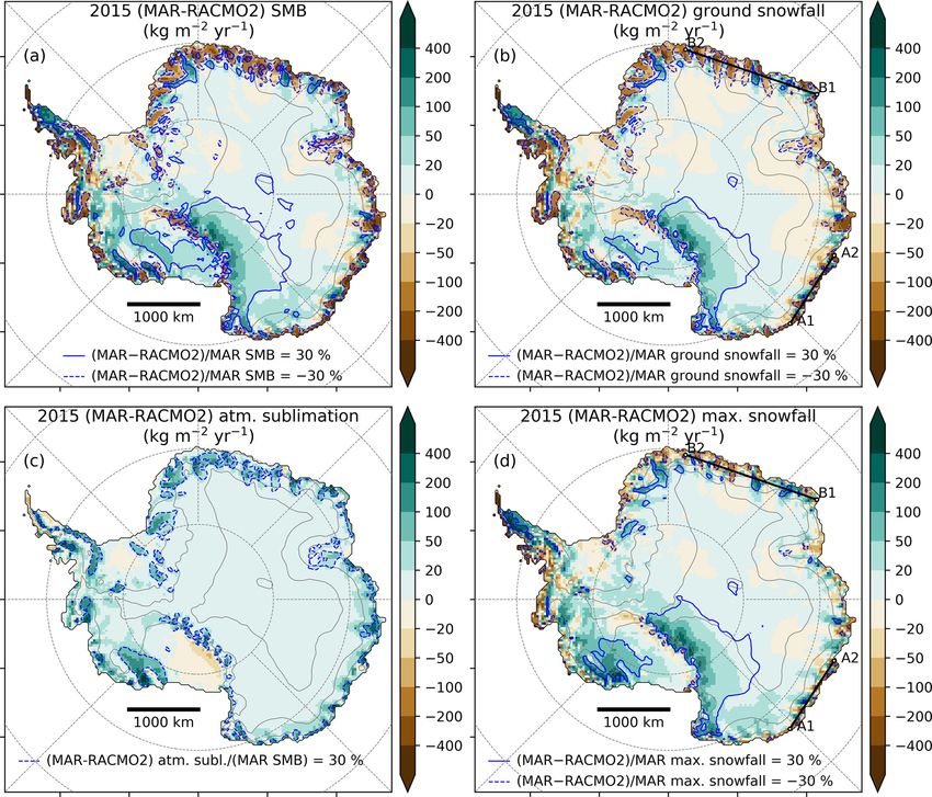
The large spatial Antarctic SMB gradients, shown in Fig. 1a Syowa–Dome F. We related these fluctuations to drifting
as modelled by MAR forced by ERA-Interim for the pe- snow transport. Indeed, the snow eroded from the snowpack
riod 1979–2015, coincide with a strong interannual variabil- is loaded into the atmosphere, where it can sublimate and be
ity (Fig. 1b), expressed by a standard deviation of ∼ 22 % transported by the wind. Katabatic winds blowing on the sur-
of the mean SMB on average over the ice sheet (Fig. 1c). face of the ice sheet result from the downslope gravity flow
MAR SMB shows no systematic spatial bias (Fig. 1d), with of cold, dense air. As a consequence, the surface wind diver-
a mean bias of 6 kg m−2 yr−1 (4 % of the mean observed gence, which drives the snowdrift mass transport, is strongly
SMB), as well as a very strong correlation with the ob- related to the curvature of the topography, and both have
served SMB (R 2 = 0.83, p value < 0.01, computed on the similar spatial patterns (shown in Fig. S9). This is because
logarithm of SMB values, as SMB distributions are log- slopes becoming steeper (crests, positive curvature) will lead
normal). RACMO2 shows similar performance (mean bias to wind speed acceleration (positive wind divergence), and
The Cryosphere, 13, 281–296, 2019 www.the-cryosphere.net/13/281/2019/
C. Agosta et al.: Antarctic SMB using MAR                                                                                                                                         285

Table 1. Sectors extracted from the GLACIOCLIM-SAMBA database.

       Sector name                              Sector type             No. of          No. of        Year range         Elevation range (m a.s.l.)           Ref.
                                                                         obs.        grid cells
       Marie Byrd Land                          Radar transects           6615               57       1980–2009                             973–1873          1
       Ross–Marie Byrd Land                     Scattered                   72               51       1950–1991                              37–1995          2,3,4
       Victoria Land                            Scattered                   60               40       1951–2006                            1804–3240          5,6,7
       Dumont d’Urville–Dome C                  Transect                   116               24       1955–2010                             633–3240          5,8,9,10
       Law Dome–Wilkes Land                     Transect                   382               32       1973–1986                             801–2232          11
       Zhongshan–Dome A                         Transect                   583               40       1994–2011                            1031–4081          12,13
       Mawson–Lambert Glacier                   Transect                   515               36       1990–1995                            1883–2924          14
       Syowa–Dome F                             Transect                   507               38       1955–2010                             584–3803          15
       Princess Elisabeth                       Transect                    58                6       2009–2012                              47–1071          16
       Dronning Maud Land                       Scattered                  376              104       1955–2008                            1753–3741          17,18,19,20

     1 Medley et al. (2014). 2 Clausen et al. (1979). 3 Venteris and Whillans (1998). 4 Vaughan et al. (1999). 5 Magand et al. (2007). 6 Frezzotti et al. (2004). 7 Frezzotti
     et al. (2007). 8 Pettré et al. (1986). 9 Agosta et al. (2012). 10 Verfaillie et al. (2012). 11 Goodwin (1988). 12 Ding et al. (2011). 13 Wang et al. (2016). 14 Higham and
     Craven (1997). 15 Wang et al. (2015). 16 GLACIOCLIM-BELARE. 17 Picciotto et al. (1968). 18 Mosley-Thompson et al. (1995). 19 Mosley-Thompson et al. (1999).
     20 Anschütz et al. (2011).

Figure 1. MAR SMB for the period 1979–2015: (a) mean annual SMB, with coloured dots showing the observed SMB values (shared
colour scale); (b) standard deviation of annual SMB; (c) standard deviation divided by mean annual SMB; (d) difference between MAR and
observed SMB on MAR grid cells, following the methodology detailed in Sect. 2.2.2. Magenta dots in panels (b) and (c) show the location
of SMB observations. Solid grey lines are contours of surface height every 1000 m a.s.l. Latitude circles are −60, −70, and −80◦ S, and
longitude lines are from 145◦ W to 145◦ E by steps of 45◦ .

thus to drifting snow export (mass loss), whereas slopes be-                                   To test our hypothesis, we computed the mean curvature
coming more gentle (valleys, negative curvature) will lead                                   of the MAR 35 km × 35 km elevation field. In Fig. 3, we
to wind speed deceleration (negative wind divergence), and                                   notice that both RCMs commonly exhibit an excess of ac-
thus to drifting snow deposit (mass gain).                                                   cumulation on crests and a deficit of accumulation in val-

www.the-cryosphere.net/13/281/2019/                                                                                            The Cryosphere, 13, 281–296, 2019
286                                                                                      C. Agosta et al.: Antarctic SMB using MAR

Figure 2. Modelled vs. observed SMB for sectors and transects as detailed in Table 1. RACMO2 outputs are bilinearly interpolated to the
MAR grid. SMB values are first averaged on MAR grid cells (Sect. 2.2.2) then along a chosen grid direction (Fig. S2) or by elevation bins.
Distance along the transect starts at the coast. Uncertainty of observed SMB (grey shaded area) is the standard deviation of observations
contained in each grid cell (sub-grid variability), estimated as a function of the mean observed SMB (see Fig. S3). Despite SMB values
corresponding to grid cell averages, we display one marker for each observation, with the x axis corresponding to the observation location
along the transect or elevation. For observed SMB plots, markers with white faces are for bins containing fewer than 10 observations and
black faces for bins containing more than 10 observations. Magenta bands mark grid cells in which more than 15 % of precipitation sublimates
in the katabatic layers according to Grazioli et al. (2017). The map shows the main Antarctic basins: Antarctic Peninsula in purple, West
Antarctic ice sheet in green, and East Antarctic ice sheet in orange. Ice shelves are mapped in blue and grounded islands in red, and the blue
line shows the location of the grounding line.

leys, in the range of ±40 kg m−2 yr−1 . To quantify this cur-            used as a proxy for wind divergence, as they are consistent
vature effect, we correlate MAR SMB bias (1SMB) with the                 with the Coriolis wind deflection westward of the topography
curvature. For each transect, we apply a constant shift of ±             gradient (detailed in Fig. S11). After applying those shifts,
one grid cell to the curvature in order to find the maximum              we find that the difference between modelled and observed
correlation with 1SMB. For three out of the four transects,              SMB (kg m−2 yr−1 ) is scaled to approximately 3700 ± 1100
we find only one shift for which the correlation is signifi-             (106 kg m−1 yr−1 ) times the curvature (10−6 m−1 ), with a
cant, and for the remaining transect (Syowa–Dome F) we                   significant relationship (R 2 = 0.41, Fig. 4a), when the mean
find no significant correlation (Fig. S10). The sign and the             annual 10 m wind speed (ws10 ) is greater than 7 m s−1 . For
amplitude of those shifts are in line with curvature being               lower wind speed (ws10 < 7 m s−1 ), we no longer observe

The Cryosphere, 13, 281–296, 2019                                                                www.the-cryosphere.net/13/281/2019/
C. Agosta et al.: Antarctic SMB using MAR                                                                                           287

Table 2. Antarctic integrated SMB on average for 1979–2015 ± 1 standard deviation of annual values, in gigatonnes per year. Antarctic ice
sheet (AIS) and basin geometry are based on Rignot basins (Shepherd et al., 2018), shown in Fig. 2. RACMO2 is bilinearly interpolated
on the MAR grid and the same mask is applied to both models, with area given for this mask. SMB is computed as follows: MAR SMB =
snowfall + rainfall − surface snow sublimation − run-off; RACMO2 SMB = snowfall + rainfall − surface snow sublimation − drifting
snow sublimation − drifting snow transport − run-off.

        Basin                  Area (106 km2 )    Component (Gt yr−1 )         MAR (ERA-Interim)       RACMO2 (ERA-Interim)
        Total AIS                        13.41    SMB                                   2200 ± 115                   2177 ± 107
        w/o peninsula                             Snowfall                              2306 ± 111                   2339 ± 107
                                                  Rainfall                                   6±1                          2±1
                                                  Surface snow sublimation                111 ± 10                       57 ± 4
                                                  Drifting snow sublimation                      –                      101 ± 5
                                                  Drifting snow transport                        –                        5±0
                                                  Run-off                                    1±1                          1±1
                                                  Melt                                     40 ± 20                      68 ± 30
        Total AIS                        13.83    SMB                                   2517 ± 111                   2516 ± 105
        Grounded AIS                     12.04    SMB                                   1923 ± 100                    1857 ± 94
        w/o peninsula                             Snowfall                               1995 ± 97                    1987 ± 94
                                                  Surface snow sublimation                  77 ± 8                       39 ± 3
                                                  Drifting snow sublimation                      –                       87 ± 4
        Grounded AIS                     12.27    SMB                                    2120 ± 99                    2068 ± 93
        Grounded East AIS                 9.77    SMB                                    1170 ± 89                    1121 ± 80
                                                  Snowfall                               1245 ± 87                    1225 ± 82
                                                  Surface snow sublimation                  77 ± 6                       34 ± 3
                                                  Drifting snow sublimation                      –                       66 ± 4
        Grounded West AIS                 2.11    SMB                                      675 ± 62                    643 ± 62
                                                  Snowfall                                 675 ± 61                    668 ± 62
                                                  Surface snow sublimation                    1±3                         4±1
                                                  Drifting snow sublimation                       –                      20 ± 2
        Grounded islands                  0.16    SMB                                        78 ± 7                       93 ± 8
        Grounded peninsula                0.23    SMB                                      198 ± 26                    211 ± 27

any relationship between model bias in SMB and curvature               the smooth SMB gradient is independent of the temperature
(horizontally aligned squares in Fig. 4a). This is consistent          (Fig. S13).
with the drifting snow transport process, which requires the              Consequently, we propose that drifting snow transport
wind speed to reach threshold values for the erosion to be             fluxes (dstr ) not resolved by MAR can be estimated as
initiated (Amory et al., 2015).                                        a scaling of curvature depending on wind speed: dstr =
   Hence, a large part of the discrepancies between modelled           α(ws10 ) · curvature (Fig. 4b). The scaling factor α(ws10 ) de-
and observed SMB are explained by surface curvature when               pends on wind thresholds to simulate the transition between
wind speed is sufficiently high, which we relate to the unre-          no drifting snow transport for low wind speed (α = 0 for
solved drifting snow transport in MAR. We are able to catch            ws10 < 5 m s−1 ) and drifting snow transport scaled to cur-
the drifting snow transport signal because drifting snow sub-          vature for high wind speed (α = 3700 106 kg m−1 yr−1 for
limation is negligible for the four studied transects, as they         ws10 > 9 m s−1 ), with a linearly increasing scaling factor
are located at high elevation, above 2000 m above sea level            between 5 and 9 m s−1 for a smooth transition around the
(a.s.l.), where the cold atmosphere has a low capacity to be           7 m s−1 wind threshold defined above. That estimate of drift-
loaded with moisture (see detailed analysis in Fig. S12). The          ing snow transport fluxes shows little sensitivity to the choice
moisture holding capacity of the atmospheric boundary layer            of the wind thresholds and of the scaling factor (see fluxes
is an upper bound for drifting snow sublimation and quickly            summed over the ice sheet for different thresholds and scal-
tends to zero when the mean air temperature decreases be-              ing factors in Table S2). The spatial pattern of drifting snow
low −30◦ C, which is the case along most of the transects,             transport we obtain is comparable to the one simulated by
whereas the amplitude of observed SMB fluctuations around              RACMO2 (Fig. 4c), except that it gives fluxes more than 3
                                                                       times larger than in RACMO2 (Table S2, and note the differ-

www.the-cryosphere.net/13/281/2019/                                                             The Cryosphere, 13, 281–296, 2019
288 C. Agosta et al.: Antarctic SMB using MAR Figure 3. Annual mean 10 m wind speed, curvature of elevation, and modelled SMB minus observed SMB for the four long transects: (a) Low Dome–Wilkes Land, (b) Zhongshan–Dome A, (c) Mawson–Lambert Glacier, and (d) Syowa–Dome F. Blue lines and colour shading are for MAR (ERA-Interim) outputs and red lines are for RACMO2 (ERA-Interim) outputs. Values are computed as in Fig. 2. ent colour map scales between Fig. 4b and c). The drifting tion in MAR than in RACMO2 (Table 2 and Fig. S6). How- snow transport estimate consists in a redistribution of mass ever, drifting snow sublimation is a potentially larger mass with negligible net mass loss over the AIS (total AIS mass sink than surface snow sublimation, as drifting snow particles gain of ∼ 75 Gt yr−1 and total AIS mass loss of ∼ 80 Gt yr−1 ; are continuously ventilated and fully exposed to the ambient see Table S2). air. Consequently, by accounting for drifting snow in MAR Our drifting snow transport estimate gives a good con- we expect that the drifting snow sublimation mass sink could straint for drifting snow fluxes above 2000 m a.s.l., where be enhanced at the expense of surface snow sublimation at low temperatures induce negligible atmospheric sublimation. the ice sheet margins. As drifting snow transport is proportional to the amount of snow in suspension in the atmosphere, quantifying this 3.3 Sublimation of precipitation in low-level flux also enables us to constrain the amount of snow eroded atmosphere from the snowpack to the atmosphere, which drives drift- ing snow sublimation fluxes at lower elevation. This is of As described above, MAR and RACMO2 RCMs forced with importance as drifting snow sublimation is a much larger ERA-Interim simulate similar spatial patterns for SMB com- mass sink than drifting snow transport over the whole ice pared to observations (Fig. 2). However, at the ice sheet sheet (Palm et al., 2017; Lenaerts et al., 2012a) but is still scale, MAR and RACMO2 SMB show regional discrepan- poorly constrained because observations are very scarce be- cies (shown in Fig. 5a for 2015, and similar to the 1979–2015 low 2000 m a.s.l. where it occurs. mean shown in Fig. S5a), which are primarily the result of Drifting snow sublimation included in RACMO2 and not differences in simulated snowfall rates (Figs. 5b and S5b). in MAR moistens the surface atmospheric layers, conse- We notice that areas where MAR snowfall is much lower quently reducing the sublimation at the surface of the snow- than RACMO2 snowfall (Fig. 5b, blue dashed lines) coincide pack. This might explain the stronger surface snow sublima- almost exactly with the pattern of precipitation that is able to The Cryosphere, 13, 281–296, 2019 www.the-cryosphere.net/13/281/2019/
C. Agosta et al.: Antarctic SMB using MAR                                                                                               289

Figure 4. (a) Difference in SMB by grid cell (1SMB) between MAR (ERA-Interim) and observations for four transects (Law Dome–Wilkes
Land, Zhongshan–Dome A, Mawson–Lambert Glacier, and Syowa–Dome F) vs. surface curvature on MAR grid. Curvature is shifted by ±
1 grid cell according to the maximum correlation with 1SMB (Fig. S10). Linear regression through the origin is plotted with a pink dashed
line. We excluded the regression of two outliers (dots with black outlines) and seven data for which MAR annual 10 m wind speed is lower
than 7 m s−1 (squares with black outlines). (b) Estimate of mean annual drifting snow transport based on a scaling of the curvature: drifting
snow transport (kg m−2 yr−1 ) = α (106 kg m−1 yr−1 ) × curvature (10−6 m−1 ), with α = 0 kg m−1 yr−1 for wind speed lower than 5 m s−1 ,
α = 3700 106 kg m−1 yr−1 for wind speed greater than 9 m s−1 , and α linearly increasing as a function of wind speed in between, around the
7 m s−1 wind speed threshold. Wind speed is the annual mean of 10 m wind speed modelled by MAR (ERA-Interim). Coloured dots show
the difference between MAR SMB and observed SMB with the same colour scale. (c) Mean annual drifting snow transport flux in RACMO2
on average for 1979–2015 (kg m−2 yr−1 ). Coloured dots show the difference between MAR SMB and observed SMB with the same colour
scale.

sublimate in the low-level atmosphere according to Grazioli              mum snowfall and the ground snowfall in each atmospheric
et al. (2017). In that study, the amount of atmospheric sub-             column, as in Grazioli et al. (2017). The same was done for
limation is quantified for the year 2015 using atmospheric               RACMO2. We find that the atmospheric sublimation simu-
modelling constrained with precipitation radar observations.             lated by MAR (363 Gt for the year 2015 over the grounded
Atmospheric sublimation happens because the katabatic sur-               ice sheet) is higher than estimated in Grazioli et al. (2017)
face air flux, moving from highly elevated inland plateau to-            (299 Gt after interpolation on the same mask) and much
ward sea level, is subject to adiabatic compression when it              higher than simulated by RACMO2 (128 Gt, Fig. 5c). A ma-
moves downslope. This compression induces an increase in                 jor difference between MAR and RACMO2 is the advection
air temperature, which reduces relative humidity and drives              of precipitation in the atmosphere: in MAR, precipitating
sublimation rates in the lower troposphere (∼ first 1000 m               particles are explicitly advected through the atmospheric lay-
above the ground), enhanced in the katabatic channels at the             ers until they reach the surface, while in RACMO2, precipita-
ice sheet margins.                                                       tion is added to the surface without horizontal advection, and
   To deepen this analysis, we re-ran MAR for the year 2015              is able to interact with the atmosphere only in a single time
in order to save the full atmosphere snowfall fields. From               step (6 min in this simulation). Consequently, atmospheric
the daily 3-D snowfall amounts, we derived the atmospheric               sublimation is likely to be underestimated in RACMO2.
sublimation amount from the difference between the maxi-

www.the-cryosphere.net/13/281/2019/                                                                The Cryosphere, 13, 281–296, 2019
290                                                                                   C. Agosta et al.: Antarctic SMB using MAR

Figure 5. The four maps show mass fluxes in kg m−2 yr−1 for the year 2015. (a) Difference in SMB between MAR and RACMO2. Blue
lines delimitate areas where the SMB difference is 30 % greater than MAR SMB, with solid lines when MAR is greater than RACMO2 and
dashed lines when MAR is lower than RACMO2. (b) Same as (a) but for the snowfall amounts at the ground. (c) Same as (a) but for the
sublimation of precipitation in the atmospheric layers. (d) Same as (a) but for the maximum snowfall amount (equal to ground snowfall plus
atmospheric sublimation). Locations of transects A1–A2 and B1–B2 extracted in Fig. 6 are shown in panels (b) and (d).

   We conclude, in agreement with Grazioli et al. (2017), that         3.4   Precipitation formation and advection
atmospheric sublimation is a major mass sink at the ice sheet
margins in MAR, as for the year 2015 it represents 16 % of
the snowfall loaded on the grounded ice sheet (12 % in Grazi-          Differences between MAR and RACMO2 snowfall fields are
oli et al., 2017) and 26 % for areas below 1000 m a.s.l. (17 %         strongly reduced when considering the maximum snowfall
in Grazioli et al., 2017).                                             amounts (before sublimation in the low-level atmosphere)
   It is noticeable that very few SMB observations are avail-          rather than the ground snowfall amounts (Fig. 5b and d).
able in areas where Grazioli et al. (2017) identify low-level          However, MAR snowfall rates generally exceed those sim-
sublimation, marked by magenta bands in Fig. 2. Except                 ulated by RACMO2, by more than 30 % on the lee side of
for Ross–Marie Byrd Land, the only other areas where low-              the West AIS (Marie Byrd Land toward Ross ice shelf), on
level sublimation is greater than 15 % of the total precipita-         the lee side of the Transantarctic Mountains (Victoria Land),
tion as defined by Grazioli et al. (2017) are close to Dumont          and close to crests at the ice sheet margins. MAR maximum
d’Urville (coastal Adélie Land) and to Syowa (coastal Dron-            snowfall rates are lower than simulated by RACMO2 wind-
ning Maud Land). In those areas the SMB amount is indeed               ward of topographic barriers and in valleys at the ice sheet
larger in RACMO2 than in MAR and in observations. Both                 margins. This spatial pattern looks similar to the one obtained
RCMs overestimate SMB around 2000 m a.s.l. in Dronning                 in RACMO2 when delaying the conversion of cloud ice–
Maud Land and in Ross–Marie Byrd Land (Fig. 2), which                  water into snow–rain (Fig. 3a of van Wessem et al., 2018).
could indicate katabatic channels not being resolved enough            This change led to both ice and water clouds lasting longer
by the topography of the models.                                       in the atmosphere before precipitating and therefore being
                                                                       advected further towards the ice sheet interior (van Wessem
                                                                       et al., 2018).

The Cryosphere, 13, 281–296, 2019                                                             www.the-cryosphere.net/13/281/2019/
C. Agosta et al.: Antarctic SMB using MAR 291 Figure 6. MAR- and RACMO2-simulated fields for the year 2015, extracted with a bilinear interpolation for (left) transect A1–A1 and (right) transect B1–B2 (locations shown in Fig. 5b and d). Each panel shows MAR fields (blue lines) and RACMO2 fields (red lines) for (a) surface height, in metres above sea level; (b) maximum snowfall amounts, equal to ground snowfall plus atmospheric sublimation, in kg m−2 yr−1 ; and (c) snowfall amounts at the ground, in kg m−2 yr−1 . In (b) and (c), the thick black line is for the difference in snowfall between MAR and RACMO2 (MAR-RACMO2), with green-filled areas when MAR snowfall is larger than RACMO2 snowfall, and brown-filled areas when MAR snowfall is lower than RACMO2 snowfall (same convention as in Fig. 5); the dotted lines are for the atmospheric sublimation modelled by MAR (blue) and by RACMO2 (red), negative when it induces a decrease in precipitation; light coloured bands show crests (light blue, curvature of MAR topography greater than 0.005 10−6 m−1 ) and valleys (light yellow, curvature of MAR topography lower than −0.005 10−6 m−1 ). The thick black arrows show the main 800 hPa wind direction during cyclonic activity. For a more in-depth analysis, we extract MAR and Dome A, Dome F; see Figs. 1d and 2). Close to summits the RACMO2 snowfall rates on two transects at the ice sheet wind is low, so a missing drifting snow transport process is margins (Fig. 6), following the main wind direction during an unlikely explanation for a positive bias in SMB modelled cyclonic activities (locations shown in Fig. 5b and d). On by MAR (Fig. 4b). Over the Greenland ice sheet, MAR tends these transects the observed difference in maximum snow- to overestimate ice cores based on accumulation inland (Fet- fall between MAR and RACMO2 is largely explained by a tweis et al., 2017) while RACMO2 underestimates it (Noël phase difference in the snowfall peaks windward of the to- et al., 2018). pographic barriers, with MAR peaking closer to the crests We conclude that the differences in MAR and RACMO2 than RACMO2 (Fig. 6b). This induces a wave-like pat- snowfall patterns are very likely related to differences in tern of precipitation difference strongly related to the shape the advection of precipitation inland, which may arise from of the topography, with larger snowfall amounts in MAR (i) the different advection of precipitating particles to the than in RACMO2 just windward of crests and lower snow- ground described in Sect. 3.3, (ii) different timing of precipi- fall amounts in MAR than in RACMO2 around windward tation formation (cloud–precipitation conversion thresholds), valleys. At the ground, lower snowfall in MAR than in and/or (iii) different dynamical response to the topographic RACMO2 in valleys is amplified by low-level atmospheric forcing, caused by either different dynamical cores or the dif- sublimation, which peaks in katabatic channels (Fig. 6c). ferent resolutions (the 27 km resolution in RACMO2 better Observations do not enable us to definitively discrimi- resolves the ice sheet topography than the 35 km resolution nate one model against the other, but we observe a general in MAR). tendency for MAR to overestimate accumulation on Ross– Marie Byrd Land and close to ice sheet summits (Dome C, www.the-cryosphere.net/13/281/2019/ The Cryosphere, 13, 281–296, 2019
292                                                                             C. Agosta et al.: Antarctic SMB using MAR

4   Discussion and conclusion                                     in valleys at the ice sheet margins. As precipitating snow par-
                                                                  ticles have larger time residence in the atmosphere in MAR
In our study, we evaluate new estimates of the Antarctic SMB      than in RACMO2 (Sect. 3.3), amounts of precipitation lost
obtained with the polar RCM MAR ran for the first time for        by sublimation in katabatic channels are more than twice as
decades-long simulations at the scale of the whole AIS. We        much in MAR as in RACMO2. The remaining spatial differ-
use model settings comparable to previous MAR simulations         ences in snowfall between MAR and RACMO2 are attributed
over Greenland (Fettweis et al., 2017) but with a specific up-    to differences in advection of precipitation, with snowfall
per atmosphere relaxation and new surface snow density and        particles being likely advected too far inland in MAR.
roughness length parameterisations. We present simulations           Atmospheric sublimation represents 429 Gt yr−1 in MAR
of MAR forced by ERA-Interim, JRA-55, and MERRA-2                 over the whole AIS (peninsula excluded) for the year 2015,
for the satellite era (1979–2015) in which we can rely on re-     89 % of which is lost below 2000 m a.s.l. and 61 % below
analyses products. Remarkably, MAR forced by those three          1000 m a.s.l. This might be of importance for the mass bal-
reanalyses gives similar spatial and temporal SMB patterns.       ance of glacier drainage basins (SMB minus discharge; Rig-
We also compare MAR with the latest simulations of the            not et al., 2008; Shepherd et al., 2018), as ice streams are typ-
RCM RACMO2 forced by ERA-Interim (van Wessem et al.,              ically channel-shaped areas affected by low-level sublima-
2018). We find no significant differences between MAR and         tion of precipitation. Consequently, we note the importance
RACMO2 SMB when integrated on the AIS and its major               of saving precipitation fluxes in models at least 1300 m above
basins (Table 2).                                                 the ground for comparison with CloudSat products, but ide-
   As the dominant feature of the Antarctic SMB is its strong     ally at all model levels below 1500 m above the ground to
coast-to-plateau gradient, we extract stake transects and sec-    be able to compute sublimation of precipitation in the low-
tors with large elevation ranges from the GLACIOCLIM-             level atmospheric layers. This will become a standard output
SAMBA SMB observational dataset. We show that both                in forthcoming MAR simulations.
RCMs show similar performances when compared to ob-                  We expect that accounting for drifting snow in MAR will
servations, with a good representation of the SMB gradient        lead to significant improvements in describing the Antarctic
(Fig. 2). But more importantly, we outline and quantify miss-     SMB and surface climate, as it will enable (1) a quantifica-
ing or underestimated processes in both RCMs.                     tion of the drifting snow sublimation mass sink, (2) a more
   Along stake transects, we relate 100 km scale fluctuations     realistic representation of relative humidity and temperature
of observations around the smooth modelled SMB pattern            in the boundary layer, and (3) an explicit modelling of the
to the shape of the ice sheet captured on the 35 km × 35 km       drifting snow transport from crests to valleys. Exploring the
MAR grid. Both RCMs accumulate too much snow on crests,           impact of horizontal and vertical model resolution on drifting
and not enough snow in valleys, as a result of drifting snow      snow estimates and on sublimation of precipitation in kata-
transport fluxes not included in MAR and probably under-          batic channels will also be of importance as those processes
estimated in RACMO2 by a factor of 3 (Fig. 4). In the             are related to the shape of the ice sheet and to the advection of
RACMO2.3p2 version used here, the modified drifting snow          precipitation in the atmosphere. The accuracy of the topogra-
routine induced almost halved drifting snow transport and         phy has to be considered as well, as digital elevation models
sublimation fluxes compared to the previous RACMO2.3p1            are in constant improvement over the AIS (e.g. Slater et al.,
version (Lenaerts and van den Broeke, 2012). In a recent          2018) and should be regularly updated in climate models.
study combining satellite observation of drifting snow events
and reanalysis products, Palm et al. (2017) estimate the drift-
ing snow sublimation to be about ∼ 393 Gt yr−1 over the           Code and data availability. Python         scripts    developed
AIS, vs. 181 Gt yr−1 in RACMO2.3p1 and 102 Gt yr−1 in             for this study as well as all required data are avail-
RACMO2.3p2 (van Wessem et al., 2018). Consequently, ob-           able     at    https://doi.org/10.5281/zenodo.2548847  (Agosta,
servational constraints from our study and from Palm et al.       2019). The last version of MAR is freely distributed at
                                                                  http://mar.cnrs.fr/ (last access: 24 January 2019). Monthly
(2017) both tend to confirm that drifting snow transport
                                                                  MARv3.6.4 outputs from this study are freely available at
and sublimation fluxes are likely much larger than previous
                                                                  https://doi.org/10.5281/zenodo.2547637 (Agosta and Fettweis,
model-based estimates and need to be (better) resolved and        2019), together with the associated MAR source code. The
constrained in climate models.                                    ECMWF reanalysis ERA-Interim 6-hourly outputs were down-
   We also point out that MAR generally simulates larger          loaded from https://doi.org/10.5065/D6CR5RD9 (ECMWF,
SMB and snowfall amounts than RACMO2 inland, partic-              2009). The MERRA-2 reanalysis 6-hourly outputs were down-
ularly on the lee side of the Transantarctic Mountains and        loaded from https://disc.gsfc.nasa.gov/datasets/ (GMAO, 2015).
on crests at the ice sheet margins, whereas MAR simulates         The JRA-55 reanalysis 6-hourly outputs were downloaded
lower snowfall than RACMO2 windward of mountain ranges            from https://doi.org/10.5065/D6HH6H41 (Japan Meteorological
and promontories. Sublimation of precipitating particles in       Agency, 2013).
low-level atmospheric layers is largely responsible for the
significantly lower snowfall rates in MAR than in RACMO2

The Cryosphere, 13, 281–296, 2019                                                       www.the-cryosphere.net/13/281/2019/
C. Agosta et al.: Antarctic SMB using MAR 293
Supplement. The supplement related to this article is available in Adélie Land, East Antarctica, The Cryosphere, 9, 1373–1383,
online at: https://doi.org/10.5194/tc-13-281-2019-supplement. https://doi.org/10.5194/tc-9-1373-2015, 2015.
Amory, C., Gallée, H., Naaim-Bouvet, F., Favier, V., Vignon, E.,
Picard, G., Trouvillez, A., Piard, L., Genthon, C., and Bel-
Author contributions. CA set-up the MAR model for Antarctica lot, H.: Seasonal variations in drag coefficient over a sastrugi-
with several adaptations, performed model simulations and anal- covered snowfield in coastal East Antarctica, Bound.-Lay. Mete-
ysed model outputs and observations. CA, AO, XF, and VF de- orol., 164, 107–133, https://doi.org/10.1007/s10546-017-0242-5,
signed the study. CA, XF, HG, CA, and CK developed the MAR 2017.
model and contributed to the MAR set-up and output analyses. Anschütz, H., Sinisalo, A., Isaksson, E., McConnell, J. R., Ham-
XF and HG are the main developers of the MAR model. MRvdB, ran, S. E., Bisiaux, M. M., Pasteris, D., Neumann, T. A., and
JMvW, JTML, and WJvdB contributed to RACMO2 output analy- Winther, J.-G.: Variation of accumulation rates over the last
ses. All authors contributed to discussions in writing this paper. eight centuries on the East Antarctic Plateau derived from vol-
canic signals in ice cores, J. Geophys. Res., 116, D20103,
https://doi.org/10.1029/2011JD015753, 2011.
Competing interests. The authors declare that they have no conflict Arthern, R. J., Winebrenner, D. P., and Vaughan, D. G.: Antarctic
of interests. snow accumulation mapped using polarization of 4.3-cm wave-
length microwave emission, J. Geophys. Res., 111, D06107,
https://doi.org/10.1029/2004JD005667, 2006.
Bamber, J. L., Gomez-Dans, J. L., and Griggs, J. A.: A new 1 km
Acknowledgements. We thank Kenichi Matsuoka, Massimo Frez-
digital elevation model of the Antarctic derived from combined
zotti, and the anonymous reviewer for their constructive and
satellite radar and laser data – Part 1: Data and methods, The
insightful comments, which led to a much improved paper.
Cryosphere, 3, 101–111, https://doi.org/10.5194/tc-3-101-2009,
Cécile Agosta performed MAR simulations during her Belgian
2009.
Fund for Scientific Research (F.R.S.-FNRS) research fellowship.
Bromwich, D. H., Fogt, R. L., Hodges, K. I., and Walsh, J. E.: A tro-
Computational resources have been provided by the Consortium
pospheric assessment of the ERA-40, NCEP, and JRA-25 global
des Équipements de Calcul Intensif (CÉCI), funded by the F.R.S.-
reanalyses in the polar regions, J. Geophys. Res., 112, D10111,
FNRS under grant no. 2.5020.11. We acknowledge Jacopo Grazioli
https://doi.org/10.1029/2006JD007859, 2007.
for sharing the low-level sublimation product and his expertise
Brun, E., David, P., Sudul, M., and Brunot, G.: A numer-
on this dataset. We acknowledge Yetang Wang for sharing his
ical model to simulate snow-cover stratigraphy for op-
updated version of the GLACIOCLIM-SAMBA dataset. We
erational avalanche forecasting, J. Glaciol., 38, 13–22,
acknowledge Christophe Genthon for fruitful discussions and
https://doi.org/10.3189/S0022143000009552, 1992.
suggestions. The authors acknowledge the support from Agence
Clausen, H. B., Dansgaard, W., Nielsen, J., and Clough, J. W.: Sur-
Nationale de la Recherche Scientifique for the scientific traverses
face accumulation on Ross Ice Shelf, Antarct. J. US, 14, 68–72,
in Antarctica and the associated research on climate and surface
1979.
mass balance modelling, projects ANR-14-CE01-0001 (ASUMA)
Dee, D. P., Uppala, S. M., Simmons, A. J., Berrisford, P., Poli,
and ANR-16-CE01-0011 (EAIIST). Cécile Agosta acknowledges
P., Kobayashi, S., Andrae, U., Balmaseda, M. A., Balsamo, G.,
the support from Fondation Albert 2 de Monaco under the project
Bauer, P., Bechtold, P., Beljaars, A. C. M., van de Berg, L., Bid-
Antarctic-Snow (2018–2020).
lot, J., Bormann, N., Delsol, C., Dragani, R., Fuentes, M., Geer,
A. J., Haimberger, L., Healy, S. B., Hersbach, H., Hólm, E. V.,
Edited by: Kenichi Matsuoka
Isaksen, L., Kållberg, P., Köhler, M., Matricardi, M., McNally,
Reviewed by: Massimo Frezzotti and one anonymous referee
A. P., Monge Sanz, B. M., Morcrette, J. J., Park, B. K., Peubey,
C., de Rosnay, P., Tavolato, C., Thépaut, J. N., and Vitart, F.: The
ERA-Interim reanalysis: configuration and performance of the
data assimilation system, Q. J. Roy. Meteor. Soc., 137, 553–597,
References https://doi.org/10.1002/qj.828, 2011.
De Ridder, K. and Gallée, H.: Land surface–induced re-
Agosta, C.: Agosta et al. (2019), The Cryosphere: gional climate change in Southern Israel, J. Appl. Me-
data processing, analyses and figures, Zenodo, teorol., 37, 1470–1485, https://doi.org/10.1175/1520-
https://doi.org/10.5281/zenodo.2548848, 2019. 0450(1998)0372.0.CO;2, 1998.
Agosta, C. and Fettweis, X.: Antarctic surface mass balance with Ding, M., Xiao, C., Li, Y., Ren, J., Hou, S., Jin, B., and Sun, B.:
the regional climate model MAR (1979–2015) [Data set], Zen- Spatial variability of surface mass balance along a traverse route
odo, https://doi.org/10.5281/zenodo.2547638, 2019. from Zhongshan station to Dome A, Antarctica, J. Glaciol., 57,
Agosta, C., Favier, V., Genthon, C., Gallée, H., Krinner, G., 658–666, https://doi.org/10.3189/002214311797409820, 2011.
Lenaerts, J. T., and van den Broeke, M. R.: A 40-year ac- European Centre for Medium-Range Weather Forecasts (ECMWF):
cumulation dataset for Adelie Land, Antarctica and its ap- ERA-Interim Project, Research Data Archive at the Na-
plication for model validation, Clim. Dynam., 38, 75–86, tional Center for Atmospheric Research, Computational
https://doi.org/10.1007/s00382-011-1103-4, 2012. and Information Systems Laboratory, updated monthly,
Amory, C., Trouvilliez, A., Gallée, H., Favier, V., Naaim-Bouvet, https://doi.org/10.5065/D6CR5RD9, 2009.
F., Genthon, C., Agosta, C., Piard, L., and Bellot, H.: Compar-
ison between observed and simulated aeolian snow mass fluxes
www.the-cryosphere.net/13/281/2019/ The Cryosphere, 13, 281–296, 2019294 C. Agosta et al.: Antarctic SMB using MAR
Eisen, O., Frezzotti, M., Genthon, C., Isaksson, E., Magand, O., Gallée, H.: Simulation of the mesocyclonic activ-
van den Broeke, M. R., Dixon, D. A., Ekaykin, A., Holm- ity in the Ross Sea, Antarctica, Mon. Weather
lund, P., Kameda, T., Karlof, L., Kaspari, S., Lipenkov, V. Y., Rev., 123, 2051–2069, https://doi.org/10.1175/1520-
Oerter, H., Takahashi, S., and Vaughan, D. G.: Ground-based 0493(1995)1232.0.CO;2, 1995.
measurements of spatial and temporal variability of snow ac- Gallée, H. and Gorodetskaya, I. V.: Validation of a limited area
cumulation in East Antarctica, Rev. Geophys., 46, 26367, model over Dome C, Antarctic Plateau, during winter, Clim.
https://doi.org/10.1029/2006RG000218, 2008. Dynam., 34, 61–72, https://doi.org/10.1007/s00382-008-0499-y,
Ettema, J., van den Broeke, M. R., van Meijgaard, E., van de Berg, 2010.
W. J., Box, J. E., and Steffen, K.: Climate of the Greenland ice Gallée, H. and Schayes, G.: Development of a three-dimensional
sheet using a high-resolution climate model – Part 1: Evalua- meso-γ primitive equation model: katabatic winds simu-
tion, The Cryosphere, 4, 511–527, https://doi.org/10.5194/tc-4- lation in the area of Terra Nova Bay, Antarctica, Mon.
511-2010, 2010. Weather Rev., 122, 671–685, https://doi.org/10.1175/1520-
Favier, V., Agosta, C., Parouty, S., Durand, G., Delaygue, 0493(1994)1222.0.CO;2, 1994.
G., Gallée, H., Drouet, A.-S., Trouvilliez, A., and Krinner, Gallée, H., Trouvillez, A., Agosta, C., Genthon, C., Favier, V., and
G.: An updated and quality controlled surface mass bal- Naaim-Bouvet, F.: Transport of snow by the wind: a compari-
ance dataset for Antarctica, The Cryosphere, 7, 583–597, son between observations in Adélie Land, Antarctica, and sim-
https://doi.org/10.5194/tc-7-583-2013, 2013. ulations made with the regional climate model MAR, Bound.-
Favier, V., Krinner, G., Amory, C., Gallée, H., Beaumet, J., Lay. Meteorol., 146, 133–147, https://doi.org/10.1007/s10546-
and Agosta, C.: Antarctica-Regional Climate and Surface 012-9764-z, 2013.
Mass Budget, Current Climate Change Reports, 3, 303–315, Gallée, H., Preunkert, S., Argentini, S., Frey, M. M., Genthon,
https://doi.org/10.1007/s40641-017-0072-z, 2017. C., Jourdain, B., Pietroni, I., Casasanta, G., Barral, H., Vi-
Fettweis, X., Franco, B., Tedesco, M., van Angelen, J. H., Lenaerts, gnon, E., Amory, C., and Legrand, M.: Characterization of
J. T. M., van den Broeke, M. R., and Gallée, H.: Estimating the boundary layer at Dome C (East Antarctica) during the
the Greenland ice sheet surface mass balance contribution to fu- OPALE summer campaign, Atmos. Chem. Phys., 15, 6225–
ture sea level rise using the regional atmospheric climate model 6236, https://doi.org/10.5194/acp-15-6225-2015, 2015.
MAR, The Cryosphere, 7, 469–489, https://doi.org/10.5194/tc- Gardner, A. S., Moholdt, G., Scambos, T., Fahnstock, M.,
7-469-2013, 2013. Ligtenberg, S., van den Broeke, M., and Nilsson, J.: In-
Fettweis, X., Box, J. E., Agosta, C., Amory, C., Kittel, C., Lang, C., creased West Antarctic and unchanged East Antarctic ice dis-
van As, D., Machguth, H., and Gallée, H.: Reconstructions of the charge over the last 7 years, The Cryosphere, 12, 521–547,
1900–2015 Greenland ice sheet surface mass balance using the https://doi.org/10.5194/tc-12-521-2018, 2018.
regional climate MAR model, The Cryosphere, 11, 1015–1033, Gelaro, R., McCarty, W., Suarez, M. J., Todling, R., Molod, A.,
https://doi.org/10.5194/tc-11-1015-2017, 2017. Takacs, L., Randles, C. A., Darmenov, A., Bosilovich, M. G., Re-
Fretwell, P., Pritchard, H. D., Vaughan, D. G., Bamber, J. L., Bar- ichle, R., Wargan, K., Coy, L., Cullather, R., Draper, C., Akella,
rand, N. E., Bell, R., Bianchi, C., Bingham, R. G., Blanken- S., Buchard, V., Conaty, A., da Silva, A. M., Gu, W., Kim, G.-
ship, D. D., Casassa, G., Catania, G., Callens, D., Conway, H., K., Koster, R., Lucchesi, R., Merkova, D., Nielsen, J. E., Par-
Cook, A. J., Corr, H. F. J., Damaske, D., Damm, V., Ferracci- tyka, G., Pawson, S., Putman, W., Rienecker, M., Schubert, S. D.,
oli, F., Forsberg, R., Fujita, S., Gim, Y., Gogineni, P., Griggs, Sienkiewicz, M., and Zhao, B.: The Modern-Era Retrospective
J. A., Hindmarsh, R. C. A., Holmlund, P., Holt, J. W., Jacobel, Analysis for Research and Applications, Version 2 (MERRA-2),
R. W., Jenkins, A., Jokat, W., Jordan, T., King, E. C., Kohler, J. Climate, 30, 5419–5454, https://doi.org/10.1175/JCLI-D-16-
J., Krabill, W., Riger-Kusk, M., Langley, K. A., Leitchenkov, 0758.1, 2017.
G., Leuschen, C., Luyendyk, B. P., Matsuoka, K., Mouginot, Genthon, C., Magand, O., Krinner, G., and Fily, M.: Do cli-
J., Nitsche, F. O., Nogi, Y., Nost, O. A., Popov, S. V., Rignot, mate models underestimate snow accumulation on the Antarc-
E., Rippin, D. M., Rivera, A., Roberts, J., Ross, N., Siegert, tic plateau? A re-evaluation of/from in situ observations in
M. J., Smith, A. M., Steinhage, D., Studinger, M., Sun, B., East Wilkes and Victoria Lands, Ann. Glaciol., 50, 61–65,
Tinto, B. K., Welch, B. C., Wilson, D., Young, D. A., Xiangbin, https://doi.org/10.3189/172756409787769735, 2009.
C., and Zirizzotti, A.: Bedmap2: improved ice bed, surface and Global Modeling and Assimilation Office (GMAO):
thickness datasets for Antarctica, The Cryosphere, 7, 375–393, MERRA-2 inst6_3d_ana_Nv: 3d,6-Hourly, Instantaneous,
https://doi.org/10.5194/tc-7-375-2013, 2013. Model-Level, Analysis, Analyzed Meteorological Fields
Frezzotti, M., Pourchet, M., Flora, O., Gandolfi, S., Gay, M., Urbini, V5.12.4, Greenbelt, MD, USA, Goddard Earth Sciences
S., Vincent, C., Becagli, S., Gragnani, R., Proposito, M., Sev- Data and Information Services Center (GES DISC),
eri, M., Traversi, R., Udisti, R., and Fily, M.: New estimations https://doi.org/10.5067/IUUF4WB9FT4W, 2015.
of precipitation and surface sublimation in East Antarctica from Goodwin, I.: Ice sheet topography and surface characteristics in
snow accumulation measurements, Clim. Dynam., 23, 803–813, eastern Wilkes Land, East Antarctica, vol. 64, ANARE research
https://doi.org/10.1007/s00382-004-0462-5, 2004. notes, available at: https://books.google.com/books/about/
Frezzotti, M., Urbini, S., Proposito, M., Scarchilli, C., and Gan- Ice_sheet_topography_and_surface_charact.html?hl=fr&id=
dolfi, S.: Spatial and temporal variability of surface mass bal- SatQAAAAYAAJ (last access: 2 April 2014), 1988.
ance near Talos Dome, East Antarctica, J. Geophys. Res., 112, Grazioli, J., Madeleine, J.-B., Gallée, H., Forbes, R. M., Gen-
F02032, https://doi.org/10.1029/2006JF000638, 2007. thon, C., Krinner, G., and Berne, A.: Katabatic winds di-
minish precipitation contribution to the Antarctic ice mass
The Cryosphere, 13, 281–296, 2019 www.the-cryosphere.net/13/281/2019/You can also read