Evaluating a landscape-scale daily water balance model to support spatially continuous representation of flow intermittency throughout stream ...
←
→
Page content transcription
If your browser does not render page correctly, please read the page content below
Hydrol. Earth Syst. Sci., 24, 5279–5295, 2020
https://doi.org/10.5194/hess-24-5279-2020
© Author(s) 2020. This work is distributed under
the Creative Commons Attribution 4.0 License.

Evaluating a landscape-scale daily water balance model to
support spatially continuous representation of flow intermittency
throughout stream networks
Songyan Yu1 , Hong Xuan Do2,3,4 , Albert I. J. M. van Dijk5 , Nick R. Bond6 , Peirong Lin7 , and Mark J. Kennard1
1 Australian Rivers Institute and School of Environment and Science, Griffith University, Nathan, Queensland, Australia
2 School of Civil, Environmental and Mining Engineering, University of Adelaide, Adelaide, Australia
3 Faculty of Environment and Natural Resources, Nong Lam University, Ho Chi Minh City, Vietnam
4 School for Environment and Sustainability, University of Michigan, Ann Arbor, Michigan, USA
5 Fenner School of Environment & Society, The Australian National University, Canberra, Australia
6 Centre for Freshwater Ecosystems, La Trobe University, Wodonga, Victoria, Australia
7 Department of Civil and Environmental Engineering, Princeton University, Princeton, New Jersey, USA

Correspondence: Songyan Yu (sunny.yu@griffith.edu.au)

Received: 17 January 2020 – Discussion started: 4 February 2020
Revised: 3 September 2020 – Accepted: 2 October 2020 – Published: 12 November 2020

Abstract. There is a growing interest globally in the spatial     river network over the period of 1911–2016, using a daily
distribution and temporal dynamics of intermittently flowing      streamflow model. The daily flow model did not perform bet-
streams and rivers, and how this varies in relation to climatic   ter than the monthly flow model in quantifying flow intermit-
and other environmental factors. However, biases in the dis-      tency at a monthly time step, and model selection should de-
tribution of stream gauges may give a misleading impression       pend on the intended application of the model outputs. Our
of spatial-temporal variations in streamflow intermittency        general approach to quantifying spatio-temporal patterns of
within river networks. Here, we developed an approach to          flow intermittency is transferable to other parts of the world,
quantify catchment-wide streamflow intermittency over long        and it can inform hydro-ecological understanding and man-
time frames and in a spatially explicit manner, using readily     agement of intermittent streams where limited gauging data
accessible and spatially contiguous daily runoff data from a      are available.
national-scale water balance model. We examined the abil-
ity of the water balance model to simulate streamflow in two
hydro-climatically distinctive (subtropical and temperate) re-
gions in Australia, with a particular focus on low-flow simu-     1   Introduction
lations. We also evaluated the effect of model time step (daily
vs. monthly) on flow intermittency estimation to inform fu-       Intermittent streams that cease to flow for some period
ture model selection. The water balance model showed better       of most years are prevalent within river networks globally
performance in the temperate region characterised by steady       (Acuña et al., 2014; Datry et al., 2014). Their spatial ex-
baseflow than in the subtropical region with flashy hydro-        tent is projected to increase in regions experiencing drying
graphs and frequent cease-to-flow periods. The model tended       trends related to climate change and water extraction for hu-
to overestimate low-flow magnitude mainly due to overesti-        man uses (Larned et al., 2010). Intermittent streams have
mation of gains (e.g. groundwater release to baseflow) during     seen increasing research interest over the past decade (e.g.
low-flow periods. Modelled patterns of flow intermittency         Costigan et al., 2016; Fritz et al., 2013; Gallart et al., 2017;
revealed highly dynamic behaviour in space and time, with         Leigh et al., 2016), and there is a growing interest in con-
cease-to-flow events affecting between 29 and 80 % of the         serving these unique ecosystems. The scarcity of spatially
                                                                  explicit information on flow intermittency has been identi-

Published by Copernicus Publications on behalf of the European Geosciences Union.
5280                           S. Yu et al.: Evaluating a daily water balance model to represent streamflow intermittency

fied as one of the key issues confronting intermittent stream      monthly time step due to higher uncertainties in input data at
management (Acuña et al., 2017). Flow intermittency exerts         this finer temporal scale (Wang et al., 2011).
primary control on the transfer of energy, materials and or-          Water balance models at a daily time step have been in-
ganisms by surface water through river networks (Jaeger et         creasingly developed around the world (Lin et al., 2019;
al., 2019) and is a key driver of riverine ecosystems (Stanley     Bierkens et al., 2015). One prominent regional example is the
et al., 1997; Datry et al., 2017; Poff et al., 1997). Therefore,   Australian Water Resource Assessment Landscape (AWRA-
improved understanding of temporal and spatial patterns in         L) model (van Dijk, 2010). The AWRA-L model has been de-
flow intermittency is fundamentally important for effective        veloped by the Commonwealth Scientific and Industrial Re-
river management.                                                  search Organisation (CSIRO) and the Australian Bureau of
   Previous studies have predominantly relied on the use of        Meteorology (BoM) to simulate the terrestrial water balance
gauged streamflow data to make inferences about the dis-           across Australia at a daily time step (van Dijk, 2010; Frost
tribution of intermittent streams in many regions, includ-         et al., 2016). The model yields spatially contiguous daily
ing France (Snelder et al., 2013), Australia (Kennard et al.,      water availability values gridded at a spatial resolution of
2010b; Bond and Kennard, 2017), Spain, and North America           0.05 arcdeg spatial resolution (approximately 5 km × 5 km)
(de Vries et al., 2015). However, spatial biases in the dis-       (Frost et al., 2016). The development of such water balance
tribution of stream gauges used in such studies may give           models in Australia and other parts of the world provides the
misleading impressions of spatial patterns and the extent          potential to quantify spatial and temporal variation in runoff,
of streamflow intermittency (Snelder et al., 2013). Alterna-       and hence flow intermittency, at a daily time step. However,
tive methods for quantifying the extent of intermittent flow       this requires an effective and efficient conversion process to
include citizen observation networks supported by regular          translate gridded runoff estimates to accumulated streamflow
reports from trained volunteers (Datry et al., 2016; Turner        estimates down the river network. This is especially chal-
and Richter, 2011), the use of electrical arrays by mea-           lenging for large study areas due to lags in runoff, which
suring the electrical conductivity of the streambed (Jaeger        can influence the timing of flow peaks and rates of reces-
and Olden, 2012), development of predictive models for in-         sion. Additionally, many national-scale water balance mod-
termittent streams (González-Ferreras and Barquín, 2017),          els, including AWRA-L, were calibrated on a large domain
and deployment of unmanned aerial systems (Spence and              that covers multiple climate conditions (Viney et al., 2015),
Mengistu, 2016). These alternatives are generally appropri-        providing a best “average” response but potentially inconsis-
ate over small spatial extents and short time frames but are       tent accuracy of runoff simulations within particular climate
difficult to scale up to larger areas to quantify flow inter-      domains. As the predictive performance for ungauged basins
mittency in space and time. Satellite remote-sensing-based         strongly depends on climate settings, this compromise raises
quantification of flow intermittency (Hou et al., 2019) can        the question as to whether such models can be used to quan-
cover larger spatial extents but, for now, remains applicable      tify flow intermittency over multiple climate conditions. Al-
only to relatively large rivers (> 30 m in the case of Landsat     though substantial efforts have been made in evaluating hy-
imagery) and can be affected by factors such as vegetation         drological models in different climate conditions (Do et al.,
and cloud obstruction.                                             2020; Gudmundsson et al., 2012; Zaherpour et al., 2018; Lin
   Spatially contiguous runoff data derived from water bal-        et al., 2019), a limited number of such studies have focused
ance models provide another potential alternative to quantify      particularly on model performance during low-flow condi-
spatio-temporal variations in flow intermittency. For exam-        tions, which is particularly important for flow intermittency
ple, Yu et al. (2018) used runoff simulations obtained from        quantification.
a water balance model, WaterDyn (Raupach et al., 2009),               In this study, we sought to apply spatially contiguous daily
to generate spatially explicit and catchment-wide estimates        runoff outputs from the AWRA-L water balance model to
of streamflow intermittency, but only at a relatively coarse       quantify the spatial extent and temporal patterns of flow in-
monthly time step. Depending on the application, flow simu-        termittency. To assess the accuracy of the AWRA-L model
lations at a finer temporal scale (e.g. daily) may be necessary    for daily flow simulations, we first developed a simple
to capture the dynamic aspects of hydrological processes.          but effective technique to convert runoff to streamflow for
These kinds of simulations are important to better understand      two hydro-climatically distinctive regions. The translation of
the causes of flow intermittency at multiple spatial scales and    gridded runoff to aggregated streamflow/discharge on vec-
enable ecologically relevant characterisation of streamflow        tor river flow lines makes AWRA-L outputs more accessible
properties such as the magnitude, frequency, duration, and         to fluvial geomorphologists and ecologists, who may intend
rate of change in high- or low-flow events. However, there         to relate daily hydrologic characteristics of rivers to a broad
are few examples of studies quantifying spatial and temporal       range of physical and ecological phenomena. We further as-
variation in flow intermittency across river networks using        sessed the uncertainty of the AWRA-L model in capturing
spatially contiguous daily flow data. That is partly because       patterns of flow intermittency. Lastly, we evaluated the effect
streamflow simulation is more challenging at a daily versus        of time step (daily vs. monthly) on the relative performance
                                                                   of the model in replicating observed patterns of cease-to-flow

Hydrol. Earth Syst. Sci., 24, 5279–5295, 2020                                       https://doi.org/10.5194/hess-24-5279-2020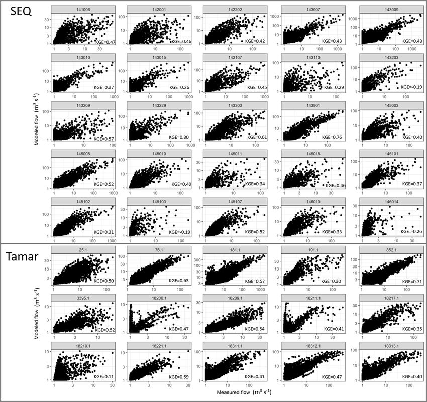
S. Yu et al.: Evaluating a daily water balance model to represent streamflow intermittency                               5281

periods at reference gauges. A previous study conducted at       3881 km2 in SEQ; 33–3294 km2 in Tamar), and flow regime
the monthly time step (Yu et al., 2018) was used to bench-       types, ranging from highly intermittent to perennial streams
mark flow intermittency estimated from the AWRA-L model.         (see results). However, the set of stream gauges used in our
                                                                 analyses under-represented the frequency of small low-order
                                                                 streams in both regions. Therefore, we regard the selected
2     Study areas                                                gauges to be representative of the range of environmental
                                                                 and hydrological conditions in the regions, except for ex-
This research was conducted in two hydro-climatically dis-
                                                                 tremely small catchments with an area < 22 km2 that likely
tinctive regions: south-east Queensland and the Tamar River
                                                                 have higher cease-to-flow occurrence.
catchment in Tasmania (Fig. 1). The south-east Queens-
land (SEQ) region is located in the eastern part of Australia
                                                                 3.2   Conversion from spatially contiguous runoff to
(Fig. 1a) and comprises five major coastal river basins with
                                                                       streamflow
a total area of 21 331 km2 (Fig. 1b). SEQ has 7229 stream
segments and their corresponding sub-catchments according
                                                                 AWRA-L is a daily 0.05◦ grid-based distributed water bal-
to the Australian Hydrologic Geospatial Fabric (Geofabric),
                                                                 ance model that is conceptualised as a small catchment. It
with a minimum upstream drainage area of 1.5 km2 . SEQ
                                                                 simulates the water flow through the landscape from the
is a region of transitional temperate to subtropical climate
                                                                 rainfall entering the grid cell through the vegetation and
(Fig. 1a) with substantial inter- and intra-annual variation
                                                                 soil and then out of the grid cell through evapotranspira-
in rainfall. The majority of rainfall and streamflow usually
                                                                 tion, surface water flow, or lateral flow of groundwater to
occurs in the summer months of January to March, often
                                                                 the neighbouring grid cells (Viney et al., 2015). AWRA-
followed by a second minor discharge peak between April
                                                                 L was calibrated and validated at the national scale dur-
and June, but high and low flows may occur at any time of
                                                                 ing its development by CSIRO and BoM, with 301 gauges
year (Kennard et al., 2007). Thus, there are a range of flow
                                                                 used for calibration and a different set of 304 gauges used
regimes, with many streams being intermittent to varying de-
                                                                 for validation (Zhang et al., 2013). Simulated daily runoff
grees. The Tamar River catchment (Tamar) is located in Tas-
                                                                 from the AWRA-L model (version 5) was downloaded from
mania, an island state off Australia’s south coast (Fig. 1a,
                                                                 BoM (http://www.bom.gov.au/water/landscape, last access:
c). It drains a catchment area of approximately 11 215 km2 ,
                                                                 28 November 2018). These data are in gridded format and
comprising over one-fifth of Tasmania’s land mass and is lo-
                                                                 require conversion to streamflow for each sub-catchment by
cated in north-east and central Tasmania. According to cli-
                                                                 aggregating the gridded runoff data with a hierarchically
mate data from BoM (http://www.bom.gov.au/climate/data,
                                                                 nested catchment to simulate streamflow throughout river
last access: 10 November 2020), Tamar is characterised by
                                                                 networks. The conversion process may or may not need to
a temperate climate condition, with rainfall relatively evenly
                                                                 use a river routing model to propagate streamflow through
distributed throughout the year.
                                                                 river networks, partly depending on the size of the catchment
                                                                 of interest (Robinson et al., 1995). If streamflow simulated
3     Data and methodology                                       with a routing model shows little difference to that without a
                                                                 routing model, then the conversion process is more efficient
3.1    Streamflow gauge data                                     without a routing model, and the readily available runoff data
                                                                 can be more accessible for potential applications, such as
Gauged daily streamflow data were sourced from the BoM           flow characterisation for ungauged stream segments. In addi-
water data website (http://www.bom.gov.au/waterdata, last        tion, a conversion process involving a routing model can be
access: 10 November 2020) and were used to assess accuracy       computationally intensive and usually requires parallel com-
of AWRA-L-modelled streamflow (Sect. 3.3) and to estimate        puting to speed up the calculations (David et al., 2011b).
an appropriate zero-flow threshold of modelled streamflow        Therefore, in this study, we applied two approaches to de-
data for quantifying patterns of streamflow intermittency        termine an effective and efficient runoff–streamflow conver-
(Sect. 3.4). A total of 25 gauges in SEQ and 15 gauges in        sion. The first approach coupled a river routing model to
Tamar were selected (Fig. 1b, c) to assess modelled stream-      the water balance model, and its effects on flow simula-
flow accuracy. These gauges had less than 0.5 % missing val-     tions are compared to the model performance of a lumped
ues over the period from 1 January 2005 to 31 December           model, which was operated without any river routing (Fig. 2).
2017 and had minimal hydrologic modification due to hu-          As the conversion process was achieved using the “catch-
man activities. A larger set of 43 gauges in SEQ (including      stats” package (https://github.com/nickbond/catchstats, last
21 of the 25 gauges used by us for streamflow validation) was    access: 10 November 2020) in the R programming language
used to estimate the zero-flow threshold for this region (see    (R Development Core Team, 2017), the second approach
Yu et al., 2018, for details of stream gauges). The gauges       was to speed up the conversion process by incorporating a
were widely dispersed throughout each study area and en-         parallel algorithm to exiting functions of that package. The
compassed a range of stream sizes, catchment areas (22–          conversion process was run on a Griffith University high-

https://doi.org/10.5194/hess-24-5279-2020                                     Hydrol. Earth Syst. Sci., 24, 5279–5295, 2020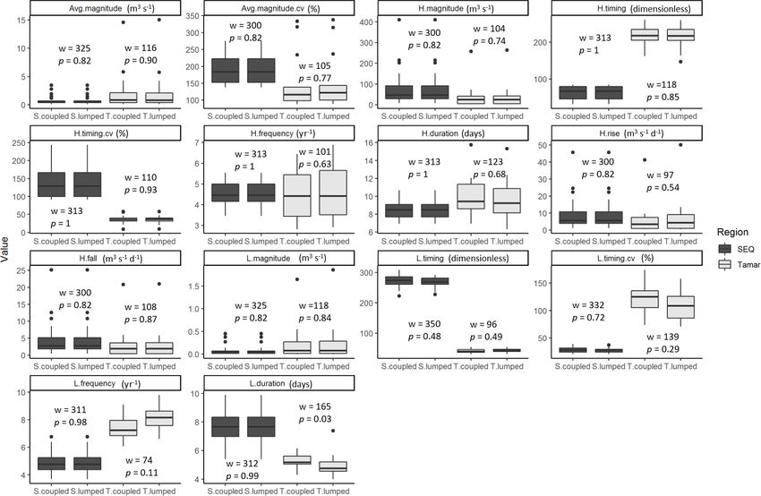
5282                             S. Yu et al.: Evaluating a daily water balance model to represent streamflow intermittency

Figure 1. Locations of the two climatically and hydrologically distinctive regions in Australia (a), south-east Queensland (SEQ) (b) and
the Tamar River catchment (Tamar) (c), with Geofabric river networks and selected stream gauges (25 and 15 gauges for SEQ and Tamar,
respectively). The climate classification in panel (a) is based on the Köppen classification system (Australian Bureau of Meteorology, 2014).

performance computing node with 12 cores and 12 GB of                    of flow regimes across average-, high-, and low-flow condi-
RAM.                                                                     tions, including flow magnitude and variability; the timing,
   The hierarchically nested catchment dataset used in this              frequency, and duration of high and low flows; and rates of
study was sourced from the Geofabric dataset (Stein et al.,              changes in flow events (Poff et al., 1997; Olden and Poff,
2014), which provides a fully connected and directed stream              2003). Calculation of these streamflow characteristics allows
network derived from the national 9 arcsec DEM and flow                  a comprehensive assessment of the effects of river routing on
direction grid (∼ 250 m resolution), and associated catch-               streamflow simulations in the two regions. We then applied
ment hierarchy at the national scale. The routing model ap-              the Wilcoxon rank sum test for each flow metric to determine
plied in this study was the Routing Application for Paral-               whether the inclusion of river routing can improve model
lel computatIon of Discharge (RAPID) model (David et al.,                accuracy based on a significance level of 5 %. We used the
2011b). RAPID solves the matrix-based Muskingum equa-                    10th and 90th percentiles of daily flows to respectively de-
tion to route flow through each stream of the river network              scribe low-flow and high-flow thresholds (Leigh and Datry,
and performs streamflow computation for every stream seg-                2016; Gudmundsson et al., 2019). The calculation process
ment of a river network, including ungauged streams. Var-                was conducted with the “hydrostats” package in the R lan-
ious water balance models have been used in combination                  guage (Bond, 2019).
with RAPID (Follum et al., 2017; Lawrence et al., 2011; Lin
et al., 2019).                                                           3.3   Accuracy assessment of modelled streamflow
   To test the effects of river routing, we first calculated a se-
ries of flow metrics (Table 1) for flow simulations from both            To evaluate overall model performance in streamflow simu-
the lumped and coupled models. The calculated flow met-                  lations, we calculated the modified Kling–Gupta efficiency
rics are commonly used to describe the critical components               (KGE; Kling et al., 2012) between the observed and mod-
                                                                         elled streamflow for all gauges in SEQ and Tamar (Eq. 1).

Hydrol. Earth Syst. Sci., 24, 5279–5295, 2020                                              https://doi.org/10.5194/hess-24-5279-2020
S. Yu et al.: Evaluating a daily water balance model to represent streamflow intermittency 5283
Figure 2. Model configurations and their applications in this study. AWRA-L runoff outputs are translated to accumulated streamflow
estimates with the river routing algorithm (coupled model) and without (lumped model). These two model configurations are applied to test
the effect of river routing on streamflow simulation accuracy. Based on the lumped model, we simulate daily streamflow throughout river
networks (daily AWRA-L) and further convert the daily stimulations to monthly outputs (monthly AWRA-L). Both simulations are used
to quantify streamflow intermittency, while results from a different monthly model (monthly WaterDyn) are used to benchmark the flow
intermittency estimates from monthly AWRA-L.
Table 1. Flow metrics used to describe average-, high-, and low-flow conditions across key components of hydrological variation. Note that
a spell independence criterion of 5 d was applied to regard periods between spells of less than 5 d as “in spell”.
Conditions Component Abbreviation Definition Units
Average flow Magnitude Avg.magnitude Mean daily flow for entire period m3 s−1
Variability Avg.magnitude.cv Coefficient of variation in mean daily flow %
High flow Magnitude H.magnitude The average annual maximum flow m3 s−1
Timing H.timing The mean Julian date of annual maximum unitless
Variability H.timing.cv Coefficient of variation in Julian date of annual maximum flow %
Frequency H.frequency Mean of annual count of spells above the 90th-percentile flow unitless
Duration H.duration Mean duration of all spells above the 90th-percentile flow days
Rate of rise H.rise Mean rate of positive changes in flow from one day to the next m3 s−2
Rate of fall H.fall Mean rate of negative changes in flow from one day to the next m3 s−2
Low flow Magnitude L.magnitude The average annual minimum flow m3 s−1
Timing L.timing The mean Julian date of annual minimum unitless
Variability L.timing.cv Coefficient of variation in Julian date of annual minimum flow %
Frequency L.frequency Mean of annual count of spells below the 10th-percentile flow unitless
Duration L.duration Mean duration of all spells below the 10th-percentile flow days
KGE is an integrated skill metric which measures the Eu- model accuracy for various components of flow regimes, in-
clidean distance between a point and the optimal point that cluding the flow metrics related to low flows. Only six of the
has the maximum correlation coefficient, zero variability 25 gauges in SEQ and three of the 15 gauges in Tamar were
error, and zero bias error between the simulated and ob- the same as those used to calibrate the AWRA-L water bal-
served streamflow (Kling et al., 2012; Gupta et al., 2009). ance model. This small overlap between the AWRA-L cali-
KGE takes values from −1 to 1: KGE = 1 indicates per- bration gauge set (n = 301) and the streamflow model valida-
fect agreement between simulations and observations, and tion gauge set (n = 25 in SEQ and 15 in Tamar) means that
KGE < −0.41 indicates that the mean of observations pro- potential overestimation of streamflow model performance is
vides better estimates than simulations (Knoben et al., 2019). likely to be minimal.
To evaluate model performance in different components of q
flow regimes, we also calculated each summary flow met- KGE = 1 − (r − 1)2 + (β − 1)2 + (γ − 1)2
ric (Table 1) for observed and modelled streamflow data at
all gauges in SEQ and Tamar and visually compared their µs CVs σs /µs
β= ; γ= = , (1)
frequency distributions. The use of KGE provides an over- µo CVo σo /µo
all assessment of AWRA-L model performance, and the flow
metrics in Table 1 are used to comprehensively evaluate the where KGE is the modified KGE statistic (dimensionless); r
is the correlation coefficient between simulated and observed
https://doi.org/10.5194/hess-24-5279-2020 Hydrol. Earth Syst. Sci., 24, 5279–5295, 20205284 S. Yu et al.: Evaluating a daily water balance model to represent streamflow intermittency
runoff (dimensionless); β is the bias ratio (dimensionless); γ gauges in the Tamar catchment had perennial flow. The envi-
is the variability ratio (dimensionless); µ is the mean runoff ronmental variables were the same as those in Yu et al. (2018)
in cubic metres per second (m3 s−1 ); CV is the coefficient and included variables related to climate (annual daily max-
of variation (dimensionless); σ is the standard deviation of imum temperature), catchment geology topography (catch-
runoff in cubic metres per second (m3 s−1 ); and subscripts s ment area, catchment average slope, and catchment average
and o refer to simulated and observed runoff values, respec- elevation), and catchment soil properties (catchment average
tively. saturated hydraulic conductivity). Regression models were
Furthermore, considering that this study aims to apply developed using all possible predictor variable combinations,
flow simulations to quantify flow intermittency, the model and we selected the “best” model for predicting zero-flow
accuracy of low-flow simulation is particularly important. duration based on the corrected Akaike’s information crite-
The study period (1 January 2005–31 December 2017) was rion (AICc) (Hurvich and Tsai, 1989). To estimate the pre-
considered sufficient to assess low flows. The 13-year study diction error of the selected model, we applied leave-one-out
period is close to a discharge record length of 15 years, which cross-validation on the selected 43 gauges and reported pre-
Kennard et al. (2010a) concluded is sufficient to enable ac- diction error (R 2 ) to estimate the model prediction perfor-
curate estimation of low-flow metrics. In addition, our study mance. Regression model development and cross-validation
period begins in the middle of the Australian Millennium were conducted with the MuMIn and boot packages in R (R
drought (2001–2009) and includes a significant low-flow pe- Development Core Team, 2017). Regression analyses were
riod. A preliminary analysis showed that AWRA-L-modelled performed on all combinations of predictor variables, and
streamflow was sensitive to rainfall events, relative to the re- the best model with the lowest AICc (−54.2) retained five
sponse of observed flow (Fig. 3). This finding indicates that covariates, including annual daily maximum temperature,
over-responsiveness of AWRA-L to rainfall may potentially catchment area, slope, average elevation, and average satu-
contribute to overestimation of low flow. We hypothesised rated hydraulic conductivity. The developed predictive model
that this over-responsiveness is partly due to overestimation showed a good model fit with an adjusted R 2 of 0.71, and
of in situ gains to low-flow discharge (e.g. groundwater re- the leave-one-out cross-validation on the regression model
lease to baseflow) as well as underestimation of transmis- showed relatively good model performance with an average
sion losses (e.g. depression filling and evapotranspiration) R 2 of 0.64. We checked for spatial autocorrelation of the re-
during water movement through various flow paths in the gression model residuals (as recommended by Dormann et
stream network (Davison and van der Kamp, 2008). Given al., 2007) and found they were not significantly autocorre-
that we do not have access to the AWRA-L model to di- lated (Moran’s I = −0.06, p = 0.69). Examination of spatial
rectly adjust model parameters, we instead compared the ob- residual maps further supported this conclusion, with no spa-
served and modelled low-flow magnitude at all gauges in the tial trends in model residuals apparent.
two study areas along the gradient of their catchment areas Next, we used the predictive models to extrapolate esti-
(22–3881 km2 in SEQ; 33–3294 km2 in Tamar) to test this mates of overall flow intermittency (in terms of the propor-
hypothesis. We expect that (1) if the difference in low-flow tion of days with zero flow) to each segment throughout the
magnitude occurs at all gauges, then low-flow overestima- river network. Finally, for each segment, the time series of
tion can be at least attributed to the overestimation of gains daily runoff was truncated (flows below the threshold were
to low-flow discharge. Alternatively, (2) if the difference in set to “0”) by adopting an appropriate threshold of “zero
low-flow magnitude occurs towards the downstream of the flow” that preserved the proportion of days with flow as es-
catchment, then low-flow overestimation may be related to timated in the previous step. The adopted thresholds ranged
underestimation of transmission losses. from 0 to 1.668 m3 s−1 , with a median value of 0.002 m3 s−1 .
We recognise several sources of uncertainty in our approach
3.4 Quantifying flow intermittency using spatially to estimating the zero-flow thresholds. The unexplained vari-
contiguous flow simulations ation in the predictive model may be due to the limited num-
ber of environmental attribute covariates used in the model
Given the fact that water balance models often over-predict and hence ability to adequately represent the range of envi-
the magnitude of very low flows due to the difficulties of ronmental processes that influence streamflow intermittency.
quantifying hydrological processes influencing low-flow dis- Additional uncertainty in model predictions may arise be-
charge (Ye et al., 1997; Smakhtin, 2001; Staudinger et al., cause the distribution of stream gauges used for model cal-
2011), we adopted the same method used in Yu et al. (2018) ibration under-represented the frequency of extremely small
to estimate a threshold of zero flow from the model that re- catchments that likely had higher cease-to-flow occurrence.
lated measured zero-flow duration at each gauge to catch- Based on the modelled daily streamflow from AWRA-L,
ment environment variables. We used linear regression to we calculated annual flow intermittency as the number of
model the mean annual zero-flow duration (daily time step) at zero-flow days per year over the period of 2005–2016. To
each gauge as a function of catchment environment variables. evaluate the effect of time step (daily vs. monthly) on the rel-
This regression analysis was only conducted in SEQ as most ative performance of AWRA-L in replicating observed pat-
Hydrol. Earth Syst. Sci., 24, 5279–5295, 2020 https://doi.org/10.5194/hess-24-5279-2020S. Yu et al.: Evaluating a daily water balance model to represent streamflow intermittency 5285
Figure 3. Comparison of the observed and modelled hydrograph with the rainfall time series at gauges 143010 in SEQ and 181.1 in Tamar.
The over-responsiveness of the model to rainfall is illustrated in the noticeable increase in modelled streamflow when a rainfall event occurred,
while there is no obvious increase in observed streamflow. Rainfall data were sourced from the AWRA-L input.
terns of cease-to-flow periods, we compared model outputs 4 Results
with those derived from a monthly water balance model –
the WaterDyn model (Fig. 2). Monthly flow intermittency es- 4.1 Negligible effects of river routing on daily flow
timated from WaterDyn was thus used to benchmark results simulations
from the monthly AWRA-L. To do this, we aggregated daily
outputs to a monthly time step (termed “monthly AWRA-L” The lumped and coupled (i.e. with routing) models using
hereafter, Fig. 2). We tried two different aggregation meth- AWRA-L-simulated runoff were run in both SEQ and Tamar,
ods. One considered that the flows for a month were zero and produced similar values for various flow metrics between
when at least one day in that month had zero flow (termed the lumped and coupled models in both regions (Fig. 4; p val-
“monthly AWRA-L_01” hereafter), and the other considered ues were greater than 0.50 for most flow metrics based on the
that all days in a month must have zero flow for that month Wilcoxon test results). There were noticeable but not statis-
to be zero (termed “monthly AWRA-L_30” hereafter). These tically significant differences for two flow metrics related to
two methods together should provide both upper and lower low flows (the variability in timing and the frequency of low-
bounds of comparing daily and monthly models in estimat- flow spells), and only the duration of low-flow spells was sta-
ing flow intermittency. The WaterDyn model was developed tistically significant (p = 0.03). These results suggested that
to provide monthly spatially contiguous water balance data the routing algorithm has nearly negligible effects on flow
at the Australian continental scale by CSIRO and BoM with simulations in our study areas, which is reasonable because
a similar model structure to AWRA-L (Raupach et al., 2018), of the small size of the two watersheds. Therefore, in the sub-
and it has been used to quantify the spatial and temporal pat- sequent analysis, we only used the results from the AWRA-L
terns of flow intermittency in SEQ following similar meth- lumped model as it is relatively less computationally inten-
ods to this study (Yu et al., 2018). Modelled flow intermit- sive and was able to maintain a comparable model perfor-
tency from all three sources (i.e. daily and monthly AWRA- mance to that of the coupled model taking into account the
L, and monthly WaterDyn) was also tested against the mea- routing effect.
sured flow intermittency derived respectively from daily and
monthly observed streamflow data at gauged locations in
4.2 Accuracy assessment of modelled streamflow in
SEQ.
SEQ and Tamar
Taking advantage of the modelled long-term runoff data
from AWRA-L over the period of 1911–2016, we further
The overall accuracy of streamflow estimated by the AWRA-
quantified spatial and temporal dynamics of flow intermit-
L lumped model (referred to as “modelled streamflow” in this
tency for every stream segment within SEQ, and compared
section) was evaluated for 25 gauges in SEQ and 15 gauges
the results with those from the WaterDyn model over the
in Tamar. Results suggested a fair to good explanatory value
same period (Yu et al., 2018). The spatial pattern of flow in-
across all gauges (Fig. 5). The KGE values varied across the
termittency was represented by the mean annual number of
25 gauges in SEQ, ranging from −0.19 (gauge no. 145103)
zero-flow days across the period of 1911–2016 for AWRA-L
to 0.76 (gauge no. 143901), with a median value of 0.42,
and by the mean annual number of calendar months for Wa-
while the model generally performed better in Tamar and the
terDyn. The temporal pattern of flow intermittency was ex-
KGE values ranged from 0.11 (gauge no. 18219.1) to 0.71
pressed as the proportion of streams with flow intermittency
(gauge no. 852.1) across 15 gauges, with a median value of
> 30 d and 1 month (termed “intermittent streams” hereafter)
0.47 (Fig. 5). However, no significant difference was found
for AWRA-L and WaterDyn, respectively.
in the overall model performance between the two hydro-
https://doi.org/10.5194/hess-24-5279-2020 Hydrol. Earth Syst. Sci., 24, 5279–5295, 20205286 S. Yu et al.: Evaluating a daily water balance model to represent streamflow intermittency
Figure 4. Comparison of hydrological characteristics between the lumped and coupled models in SEQ and Tamar. Refer to Table 1 for
measurement description for each flow metric. Metrics are grouped according to average (Avg), high (H) and low (L) flow conditions. The
values of w statistic and associated p values are also shown to indicate whether there is any significant difference between the coupled and
lumped simulations.
climatically distinctive regions, according to the Wilcoxon gauges. There appeared to be a tendency toward larger dif-
test (w = 247, p = 0.10). ferences with increasing catchment area in SEQ but not in
Concerning model performance in simulating different Tamar (Fig. 7). The models appeared to overestimate in situ
components of flow regimes, the modelled streamflow in gains to low flow in some reaches in both regions, while
SEQ revealed a generally good match with the observed underestimating transmission losses in SEQ, suggesting that
streamflow across all high-flow metrics and the magnitude overestimation of in situ gains in AWRA-L likely contributes
of average flow, but the model tended to overestimate the to the overall overestimation of low flow in downstream
variation in the magnitude of average flow (almost 2 times catchments.
higher on average), report earlier timing of low flows, over-
estimate the frequency (48 % higher), and underestimate the 4.3 Quantifying flow intermittency using flow
duration (74 % lower) of low flows (Fig. 6). Compared to the simulations
model performance in SEQ, the flow simulations in Tamar
showed slightly better performance, predicting well not only
We calculated annual flow intermittency at gauged locations
for the high-flow metrics but also for the metrics related to
in SEQ using three sources of modelled flow (daily and
average flows (Fig. 6). However, flow simulations in Tamar
monthly AWRA-L, and monthly WaterDyn). Annual flow
also exhibited slightly earlier estimations for the timing of
intermittency calculated using daily AWRA-L flow (i.e. the
low-flow spells (13 % earlier), overestimations for low-flow
average number of cease-to-flow days per year) was tested
spell frequency (92 % lower on average), and underestima-
against annual flow intermittency estimated using observed
tion for low-flow spell duration (58 % lower) (Fig. 6).
data (Fig. 8a). The AWRA-L model displayed the poten-
Varying degrees of difference in the magnitude of low flow
tial to be used to estimate flow intermittency at a daily time
between the observed and simulation were found among the
step, with a fair match with the observed flow intermittency
Hydrol. Earth Syst. Sci., 24, 5279–5295, 2020 https://doi.org/10.5194/hess-24-5279-2020S. Yu et al.: Evaluating a daily water balance model to represent streamflow intermittency 5287 Figure 5. Scatter plots of the measured and modelled (lumped) streamflow for each gauge station in SEQ and Tamar. The modified Kling– Gupta efficiency (KGE) is presented in each panel. The x and y axes are log-transformed (log10 (x + 1)) to aid interpretation. (R 2 = 0.56) in SEQ. Nonetheless, the model tended to over- in estimating flow intermittency (R 2 = 0.53, 0.43, and 0.32 estimate flow intermittency for gauges located in relatively respectively for monthly WaterDyn, monthly AWRA-L_01, wet areas (e.g. ≤ 40 d of flow intermittency per year) while and monthly AWRA-L_30). More specifically, the Water- underestimating it for gauges located in relatively dry areas Dyn model displayed a similar estimation pattern to the daily (e.g. ≥ 40 d of flow intermittency per year). AWRA-L model: overestimation in relatively wet areas and Figure 8b shows annual flow intermittency calculated us- underestimation in relatively dry areas. By contrast, not sur- ing monthly AWRA-L flow and monthly WaterDyn flow. In prisingly, the two aggregation methods showed the upper this case, annual flow intermittency was defined as the av- and lower bounds of flow intermittency estimates from the erage number of months characterised with zero flow. The monthly AWRA-L model: monthly AWRA-L_01 overesti- WaterDyn model showed much more accuracy than the two mated flow intermittency and monthly AWRA-L_30 under- aggregation methods based on the monthly AWRA-L model estimated flow intermittency at nearly all gauges (Fig. 8b). https://doi.org/10.5194/hess-24-5279-2020 Hydrol. Earth Syst. Sci., 24, 5279–5295, 2020
5288                             S. Yu et al.: Evaluating a daily water balance model to represent streamflow intermittency

Figure 6. Variation in observed and modelled (lumped) hydrologic characteristics in SEQ and Tamar (n = 25 and 15 gauge locations,
respectively). Refer to Table 1 for measurement description for each flow metric. Metrics are grouped according to average (Avg), high (H)
and low (L) flow conditions. The y axis is on a log scale for better interpretation.

                                                                          The spatial patterns of flow intermittency derived from
                                                                       the daily AWRA-L and monthly WaterDyn flow simulations
                                                                       aligned well for the main stems and some coastal streams,
                                                                       which were predicted to flow for most of the time (Fig. 9a,
                                                                       b). There were noticeable spatial differences between model
                                                                       predictions of streamflow intermittency for low-order in-
                                                                       land streams. For example, in the western Brisbane River
                                                                       catchment and the South Coast River catchment, most in-
                                                                       land streams were predicted by the daily model to flow for a
                                                                       longer period than by the monthly model; while in the Pine
                                                                       River catchment and the Logan–Albert River catchment,
                                                                       many inland streams were predicted by the daily model to
                                                                       flow for a shorter period (Fig. 9a). Compared to the monthly
                                                                       WaterDyn model, fewer streams were predicted by the daily
                                                                       AWRA-L to experience extremely long dry events as well
Figure 7. Scatter plot of gauged catchment areas and percentage        as less than 1 month of zero flows (Fig. 9c, d). However,
difference in low-flow magnitude between the observation and sim-      more streams on average (60 and 49 % for the AWRA-L and
ulation in SEQ (solid grey triangle) and Tamar (black cross). The      WaterDyn model, respectively) were predicted to flow inter-
regression line for each region is also shown as a solid line (grey    mittently (> 30 d or > 1 month) to varying degrees in SEQ,
line for SEQ and black line for Tamar) with the regression function    which suggests that flow intermittency was prevalent in SEQ,
and R 2 value.                                                         irrespective of the water balance model used.

Hydrol. Earth Syst. Sci., 24, 5279–5295, 2020                                            https://doi.org/10.5194/hess-24-5279-2020
S. Yu et al.: Evaluating a daily water balance model to represent streamflow intermittency 5289
5 Discussion
The scarcity of information on the spatial and temporal ex-
tent of flow intermittency has been identified as a major bar-
rier for ecologists and managers to understand and protect in-
termittent stream ecosystems (Acuña et al., 2017). This bar-
rier has been partly overcome in previous studies by using
statistical models relating flow intermittency to surrounding
environmental variables (Snelder et al., 2013; Jaeger et al.,
2019; González-Ferreras and Barquín, 2017; Bond and Ken-
nard, 2017), but most of these studies focused on only the
spatial variations in flow intermittency, except for Jaeger et
al. (2019), overlooking its temporal aspects. This issue be-
comes particularly urgent in a time when flow regimes of
streams are changing worldwide, mainly in response to cli-
mate change and water extraction for human uses (Jaeger et
al., 2014; Chiu et al., 2017). Monthly runoff data have been
recently used to quantify flow intermittency for entire river
networks (Yu et al., 2018), and the current study takes one
step further to use daily runoff data in flow intermittency
estimation, which is especially needed for studies aimed at
quantifying ecological responses to short-term flow events
(e.g. frequent zero-flow events within a month). In this study,
we comprehensively examined the ability of a daily water
Figure 8. Scatter plots of the observed and modelled flow inter- balance model to simulate streamflow, with a particular fo-
mittency by the two models (AWRA-L and WaterDyn model) for cus on low-flow simulations. We also investigated how to
SEQ. Daily AWRA-L and monthly WaterDyn are derived from the better choose water balance models to estimate flow inter-
original data from the two models, while AWRA-L monthly_01 and mittency by answering the question of whether daily flow
monthly_30 are flow intermittency estimates using the two different
models outperform monthly flow models at both daily and
aggregation methods with different thresholds (1 and 30 d, respec-
monthly scales. Our study can not only inform the estimation
tively) to classify a month as zero-flowing. The solid line represents
the regression line for each model. The 1 : 1 line (dashed line) is of the spatial distribution of intermittent flow but also reveal
plotted for reference. the temporal dynamics of intermittent streams over long time
frames.
Temporally, the daily model estimated that the proportion 5.1 Efficient runoff–streamflow conversion for
of intermittent streams in SEQ varied from 29 to 80 % over eco-hydrological research
the study period (1911–2016), while the monthly model es-
timated the range to be from 3 to 80 % estimated during the Effects of river routing on daily flow simulations were found
same time span (Fig. 10). The two temporal patterns were to be negligible in SEQ and Tamar, most probably due to the
temporally correlated (r = 0.71), and similar predictions with relatively small size of the two catchments and the relatively
higher proportions of intermittent streams were estimated for short length of even the longest streams (Cunha et al., 2012).
the dry years by both models. Compared to dry years, the two This can be verified with the concept of time of concentra-
models exhibited greater differences in predictions for the tion, which is commonly used to measure the time needed
wet years, where the daily model tended to predict a higher for water to flow from the most remote point in a catchment
proportion of intermittent streams. Overall, the daily model to the catchment outlet. By following the formula for cal-
suggested a drier history in SEQ in terms of flow intermit- culating the time of concentration proposed by Pilgrim and
tency than the monthly model. The models successfully iden- McDermott (1982) that has been widely used in Australia,
tified the extensive drying associated with severe drought pe- we found the time of concentration in SEQ is around 33 h,
riods. Notably, the Widespread drought (1914–1920), WWII only slightly more than a daily time step (24 h). This illus-
drought (1939–1946), and Millennium drought (2001–2009) trates why it is difficult for a daily time-step routing model to
were all visible in both two sets of model predictions. effectively capture routing lags in our study domain. A neg-
ligible effect of river routing on flow simulations was also
observed in previous studies (David et al., 2011a). Robinson
et al. (1995) found that catchment size is a primary factor in
determining which process, the hillslope or the channel net-
https://doi.org/10.5194/hess-24-5279-2020 Hydrol. Earth Syst. Sci., 24, 5279–5295, 20205290 S. Yu et al.: Evaluating a daily water balance model to represent streamflow intermittency
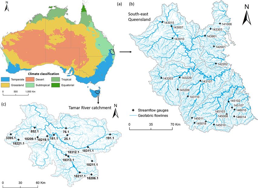
Figure 9. Comparison of the spatial pattern of average annual flow intermittency in SEQ derived from (a) daily flow simulations from the
AWRA-L model and (b) monthly flow simulations from the WaterDyn model. Stream segments in both figures are coloured using the same
frame but different units. Line thicknesses show the stream orders. Frequency distributions of variations in the total stream length for each of
12 flow intermittency classes are also shown for (c) the AWRA-L model and (d) the WaterDyn model.
work transport component, characterises lags in catchment curately simulated in the Tamar than in SEQ (the median
runoff down the river network. In areas such as SEQ and values of KGE were 0.47 and 0.42, respectively), the dif-
Tamar that have a relatively small catchment size, the inclu- ferences between the two hydro-climatically distinctive re-
sion of channel network transport contributes little to the im- gions were relatively small. Despite ongoing efforts to cali-
provement of flow simulations. The negligible effect of river brate AWRA-L against a set of reference scales distributed
routing in SEQ and Tamar allowed us to simplify the sim- across the continent (Viney et al., 2015), this finding was re-
ulation of daily flows without coupling with a river routing assuring given the much higher variability in rainfall and soil
model. Hence we were able to use existing runoff outputs moisture in SEQ, factors that typically can lead to a more
from the daily AWRA-L model. Arguably, similar opportu- non-linear streamflow response to rainfall (Poncelet et al.,
nities exist in other small catchments. 2017), which possibly undermines the ability of water bal-
ance models to reliably predict runoff (Sheng et al., 2017).
5.2 Accuracy assessment of modelled daily streamflow These results hence bode well for the application of AWRA-
in two hydro-climatically distinctive regions L outputs across diverse hydroclimatic regions.
When looking into the model performance for specific
Daily streamflow estimates showed a fair to good overall components of the flow regime, average- and high-flow met-
alignment with the observed flows in both SEQ and Tamar, rics were both modelled well in Tamar, while only high-
with all gauges showing that flow simulations were better flow metrics were modelled well in SEQ. However, in both
estimates than the mean of observations (KGE ≥ −0.41 at regions, the AWRA-L model showed poor performance in
all gauges). Interestingly, although streamflow was more ac- low-flow metrics: overestimating the frequency and under-
Hydrol. Earth Syst. Sci., 24, 5279–5295, 2020 https://doi.org/10.5194/hess-24-5279-2020S. Yu et al.: Evaluating a daily water balance model to represent streamflow intermittency 5291
Figure 10. Comparison of intra-annual variation of the proportion of intermittent streams in length from 1911 to 2016 across SEQ, derived
from streamflow simulations from the daily flow model (lumped, solid grey line) and monthly flow model (dashed grey line). Three severe
droughts in Australia were also presented as transparent grey rectangles: Widespread drought (1914–1920), WWII drought (1939–1946),
and Millennium drought (2001–2009). The time series of annual mean precipitation is shown for reference.
estimating the duration of low flows, consistent with pre- as AWRA-L has been released as a community modelling
vious studies (Costelloe et al., 2005; Ivkovic et al., 2014; system (https://github.com/awracms/awra_cms, last access:
Ye et al., 1997; Staudinger et al., 2011). This suggests that 10 November 2020), which allows co-development by the
the AWRA-L model is a generally robust model in predict- research community.
ing average and high flows but still needs some improve-
ment to better simulate low flows. Runoff generation pro-
cesses can vary substantially through space and time due 5.3 Choose appropriate water balance model to
to such factors as variations in soil depth, antecedent soil quantify spatio-temporal dynamics of flow
moisture, and groundwater connectivity, and this can influ- intermittency
ence spatio-temporal variations in low-flow characteristics,
including streamflow intermittency (Zimmer and McGlynn,
Our results suggest that the temporal resolution of analy-
2017). However, it is unknown to what extent this contributed
sis should be dictated by the resolution of input stream-
to uncertainty in the simulation of low flows and estimation
flow data. More specifically, the daily AWRA-L flow showed
in streamflow intermittency in this study. The uncertainty of
promise for estimating flow intermittency at a daily time
AWRA-L in low-flow simulations can be linked to its over-
step, while the monthly WaterDyn model was better than the
responsiveness to rainfall, partly caused by overestimation
monthly AWRA-L model in flow intermittency estimation at
of in situ gains and underestimation of transmission losses
a monthly time step. This suggests that monthly flow mod-
to low-flow discharge, as shown in SEQ. Previous studies
els can sometimes outperform daily flow models in quanti-
found that lateral flow exchange between grid cells of land
fying flow intermittency, depending on the intended tempo-
surface models (e.g. AWRA-L) plays a significant role in re-
ral resolution of the analysis. For example, daily flow mod-
distributing soil water (Kim and Mohanty, 2016), and thus
els may be appropriate for studies aimed at quantifying eco-
may improve in situ surface/subsurface runoff simulations
logical responses to short-term flow events, while monthly
(Lee and Choi, 2017). On the other hand, hydrological pro-
flow models are more suitable for research requiring the av-
cesses involved in transmission losses have been extensively
erage degree of flow intermittency at a large spatial or tem-
discussed (Jarihani et al., 2015; Konrad, 2006), and studies
poral scale, such as examining the effect of flow intermit-
have developed methods to calculate transmission losses for
tency on aquatic/streamside vegetation or species distribu-
better flow simulations (Lange, 2005; Costa et al., 2012).
tions (Stromberg et al., 2005). In addition, our study also
Therefore, low-flow simulations by AWRA-L can possibly
suggested that the suitability of a monthly model (WaterDyn)
be improved by incorporating lateral flow exchange algo-
for monthly resolution of analysis was not challenged by a
rithms and better accounting for hydrological process such as
daily model (AWRA-L) simply through aggregating daily
evapotranspiration from riparian vegetation and infiltration
streamflow simulations to a monthly time step. The aggrega-
into channel beds. This improvement is made more likely
tion methods used here applied 1 or 30 d as a threshold and,
https://doi.org/10.5194/hess-24-5279-2020 Hydrol. Earth Syst. Sci., 24, 5279–5295, 20205292 S. Yu et al.: Evaluating a daily water balance model to represent streamflow intermittency
respectively, either substantially overestimated or underesti- data from a readily accessible water balance simulation. This
mated flow intermittency. research builds upon previous studies using monthly runoff
Spatially contiguous runoff data were used in this study data, and paves the way for ecological research looking for
to quantify spatial and temporal dynamics of flow intermit- metrics of flow intermittency at a daily time step. By testing
tency, shedding light on the temporal aspect of flow inter- this approach in eastern Australia, we not only confirmed our
mittency that has been often overlooked in previous studies. previous finding that intermittent flow conditions prevailed in
Annual flow intermittency in SEQ was shown to vary signif- the majority of streams, but also provided more detailed in-
icantly from year to year, ranging from 29 to 80 % of total formation on their spatio-temporal variability at a daily time
stream length for the AWRA-L model. However, given the step. The proposed approach has potential applicability to
limited spatial resolution of the Geofabric stream network other catchments globally, but our results also highlighted
data (9 arcsec longitude–latitude resolution, with a minimum some complexities that future research should address to help
upstream drainage area of 1.5 km2 ) and hence ability to re- improve the reliability of model outputs.
solve the smallest streams, and that small streams are more
likely to be intermittent, the proportion of predicted inter-
mittent streams in SEQ may be underestimated in our study. Data availability. The data used in this study are available publicly
Although there are differences in the temporal patterns of es- online, and the access websites have been listed in the main text
timated flow intermittency between the AWRA-L and Water- where they were first mentioned.
Dyn models, neither model estimated intermittency to have
a clear trend over the past century. However, there is still the
concern about the potential shift of some perennial streams Author contributions. AIJMvD, HXD, MJK, and SY designed the
research, and SY and HXD carried it out. SY wrote the original
to intermittent streams due to climate change and intense
draft, and HXD, AIJMvD, PL, NRB, and MJK contributed to writ-
human activities, as it has been evident in several regions
ing of subsequent drafts.
where the number of low-flow and/or no-flow days is in-
creasing (King et al., 2015; Ruhí et al., 2016; Sabo, 2014).
Jaeger et al. (2014) investigated the effect of climate change Competing interests. The authors declare that they have no conflict
on flow intermittency patterns and found that annual zero- of interest.
flow days frequency were projected to increase by 27 % by
mid-century in the Lower Colorado River basin of the United
States. Research looking into projected changes in regional Acknowledgements. The project was supported by the Australian
climate regimes can provide insights into future scenarios Climate and Water Summer Institute organised by the Australian
people may face, but such research is still scarce. Energy and Water Exchange Research Initiative (OzEWEX) and
The approach developed here to generate spatially contin- partners. This research was undertaken at the NCI National Facility
uous estimates of streamflow characteristics (including flow in Canberra, Australia, which is supported by the Australian Com-
intermittency) throughout stream networks has potential ap- monwealth Government. We also gratefully acknowledge the sup-
plicability to other regions of Australia and globally. All the port of the Griffith University eResearch Services team and the use
of the high-performance computing cluster “Gowonda” to complete
data used in this study are available for the Australian na-
this research. We would like to thank the Editor Christa Kelleher
tional scale, and similar datasets also exist in other coun- for handling our submitted manuscript, and thank George Allen and
tries. For example, similar to the Geofabric data (Stein et three anonymous reviewers for their comments and suggestions that
al., 2014) used here, the National Hydrography Dataset Plus much improved the final manuscript.
(NHDPlus) and HydroATLAS (Linke et al., 2019) provide
hydrographic datasets and hydro-environmental attributes for
national (USA) and global scales, respectively. In addition, Financial support. This research has been supported by the
similar to the daily flow model AWRA-L used in this study, China Scholarship Council and Griffith University (grant
other global- and national-scale hydrologic models are also no. 201506040057) and the University of Michigan (grant
available, such as the global WaterGAP model (Döll et al., no. U064474).
2003), the community Noah land surface model (Noah-MP)
(Niu et al., 2011) in the USA, and the HYPE model (Lind-
ström et al., 2010) in Sweden. Review statement. This paper was edited by Christa Kelleher and
reviewed by George Allen and three anonymous referees.
6 Conclusions
In this study, we presented an approach to quantifying spa-
tially explicit and catchment-wide flow intermittency over
long time frames based on spatially contiguous daily runoff
Hydrol. Earth Syst. Sci., 24, 5279–5295, 2020 https://doi.org/10.5194/hess-24-5279-2020You can also read