Evaluating the simulated mean soil carbon transit times by Earth system models using observations - Biogeosciences
←
→
Page content transcription
If your browser does not render page correctly, please read the page content below
Biogeosciences, 16, 917–926, 2019
https://doi.org/10.5194/bg-16-917-2019
© Author(s) 2019. This work is distributed under
the Creative Commons Attribution 4.0 License.

Evaluating the simulated mean soil carbon transit times by Earth
system models using observations
Jing Wang1 , Jianyang Xia1,2 , Xuhui Zhou1,2 , Kun Huang1 , Jian Zhou1 , Yuanyuan Huang3 , Lifen Jiang4 , Xia Xu5 ,
Junyi Liang6 , Ying-Ping Wang7 , Xiaoli Cheng8 , and Yiqi Luo4,9
1 Zhejiang Tiantong Forest Ecosystem National Observation and Research Station, Shanghai Key Lab for Urban Ecological
Processes and Eco-Restoration, School of Ecological and Environmental Sciences, East China Normal University,
Shanghai 200241, China
2 State Key Laboratory of Estuarine and Coastal Research, Research Center for Global Change and Ecological Forecasting,

East China Normal University, Shanghai 200241, China
3 Laboratoire des Sciences du Climat et de l’Environnement, 91191 Gif-sur-Yvette, France
4 Center for ecosystem science and society, Northern Arizona University, Arizona, Flagstaff, AZ 86011, USA
5 College of Biology and the Environment, Nanjing Forestry University, Nanjing 210037, China
6 Environmental Sciences Division & Climate Change Science Institute, Oak Ridge National Laboratory,

Oak Ridge, Tennessee 37830, USA
7 CSIRO Ocean and Atmosphere, PMB 1, Aspendale, Victoria 3195, Australia
8 Wuhan Botanical Garden, Chinese Academy of Sciences, Wuhan 430074, Hubei Province, China
9 Department of Earth System Science, Tsinghua University, Beijing 100084, China

Correspondence: Jianyang Xia (jyxia@des.ecnu.edu.cn)

Received: 16 July 2018 – Discussion started: 15 August 2018
Revised: 5 February 2019 – Accepted: 15 February 2019 – Published: 27 February 2019

Abstract. One known bias in current Earth system models              showed that one ESM (i.e., CESM) has improved its τsoil
(ESMs) is the underestimation of global mean soil carbon             estimate by incorporation of the soil vertical profile. These
(C) transit time (τsoil ), which quantifies the age of the C         findings indicate that the spatial variation of τsoil is a useful
atoms at the time they leave the soil. However, it remains           benchmark for ESMs, and we recommend more observations
unclear where such underestimations are located globally.            and modeling efforts on soil C dynamics in regions limited
Here, we constructed a global database of measured τsoil             by temperature and moisture.
across 187 sites to evaluate results from 12 ESMs. The ob-
servations showed that the estimated τsoil was dramatically
shorter from the soil incubation studies in the laboratory en-
vironment (median = 4 years; interquartile range = 1 to              1   Introduction
25 years) than that derived from field in situ measurements
(31; 5 to 84 years) with shifts in stable isotopic C (13 C) or the   Carbon (C) cycle feedback to climate change is highly uncer-
stock-over-flux approach. In comparison with the field obser-        tain in current Earth system models (ESMs) (Friedlingstein
vations, the multi-model ensemble simulated a shorter me-            et al., 2006; Bernstein et al., 2008; Ciais et al., 2013; Brad-
dian (19 years) and a smaller spatial variation (6 to 29 years)      ford et al., 2016), which largely stems from their diverse sim-
of τsoil across the same site locations. We then found a sig-        ulations of C exchanges among the atmosphere, vegetation,
nificant and negative linear correlation between the in situ         and soil (Luo et al., 2016; Smith et al., 2016; Mishra et al.,
measured τsoil and mean annual air temperature. The under-           2017). Soil organic carbon (SOC) represents the largest ter-
estimations of modeled τsoil are mainly located in cold and          restrial carbon pool, which stores at least 3 times as much
dry biomes, especially tundra and desert. Furthermore, we            as the atmospheric and vegetation C reservoirs (Parry et al.,
                                                                     2007; Bloom et al., 2016). However, a 5- to 6-fold differ-

Published by Copernicus Publications on behalf of the European Geosciences Union.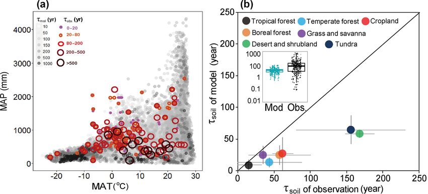
918                                                  J. Wang et al.: Evaluating the simulated mean soil carbon transit times

ence in soil C stocks among ESMs or offline global land sur-       2018). Rasmussen et al. (2016) has marked off the transit
face models has been found (Todd-Brown et al., 2013; Luo           time and mean system age in a mathematic way and further
et al., 2016). It is difficult to reduce or even diagnose this     applied it in the Carnegie–Ames–Stanford approach (CASA)
uncertainty, as many processes collectively affect the time of     model. Also, the methodological uncertainty is large, espe-
C atoms’ transit in the soil system (i.e., transit time, τsoil )   cially when these approaches are applied to estimate the τsoil
(Sierra et al., 2017; Spohn and Sierra, 2018). Some recent         of different soil fractions (Feng et al., 2016). Thus, this study
attempts at evaluating and diagnosing the modeled SOC in           mainly collects the τsoil values from the approaches of stock
ESMs have shown significant simulation uncertainties in the        over flux, 13 C changes, and lab incubations in further analy-
τsoil (Todd-Brown et al., 2013; Carvalhais et al., 2014; He et     ses.
al., 2016; Koven et al., 2017). For example, there is a 4-fold        In this study, we first construct a database from the litera-
difference in the simulated τsoil among the ESMs from the          tures which reported τsoil (Fig. 1a, Supplement on Text S1).
Coupled Model Intercomparison Project Phase 5 (CMIP5)              Then, the database is used to evaluate the simulated τsoil by
(Todd-Brown et al., 2013). A recent data-driven analysis has       the ESMs in CMIP5. The SOC τsoil values were calculated
suggested that the current ESMs have substantially underes-        under a homogenous one-pool assumption at steady state for
timated the τsoil by 16–17 times at the global scale (He et        all studies. Data from observations and the CMIP5 ensem-
al., 2016). Therefore, identifying the locations of such un-       ble were then used to calculate the τsoil based on both one-
derestimations is critical to improve the predictive ability of    pool and three-pool models. Many ESMs, e.g., CESM, have
ESMs for the terrestrial C cycle, and the construction of a        released new versions in recent years, so we also evaluate
benchmarking database of available observations is urgently        whether the simulated τsoil has been improved. In the case
needed (Koven et al., 2017).                                       of CESM, one of its major developments in soil C cycling is
   The terms of transit time, turnover time, and age of soil C     the vertically resolved soil biogeochemical scheme (Koven et
have been muddled in diagnosing the models (Sierra et al.,         al., 2013). Thus, we employ a matrix approach developed by
2017). The diagnostic times derived from observational data        Huang et al. (2017) to examine the impact of the vertically
are based on the different assumptions and mainly derived          resolved soil biogeochemical scheme on the τsoil simulated
from four approaches. The first approach is commonly de-           by CESM.
fined as “turnover time”, calculated by the division of SOC
stock by C fluxes such as net primary productivity (NPP)
or heterotrophic respiration (Rh ). It assumes the soil system     2     Materials and methods
is a time-invariant linear system in a steady state (Bolin et
al., 1973; Sanderman et al., 2003; Six and Jastrow, 2012).         2.1    A global database of site-level τsoil
The second approach is based on the shifts in stable iso-
topic C (13 C) after successive changes in C3 –C4 vegeta-          We collected the literatures that reported the τsoil based on
tion, together with additional information from the disturbed      measurements (Text S1 in the Supplement): (1) δ 13 C shifts
and undisturbed soils (Balesdent et al., 1987; Zhang et al.,       after successive changes in C3 -C4 vegetation, (2) measure-
2015). The third approach is based on simulating soil C dy-        ments of CO2 production in laboratory SOC incubation over
namics with linear models by assimilating the observational        at least 7 months, and (3) simultaneous measurements of
data from laboratory incubations of soil samples (Xu et al.,       SOC stock and heterotrophic respiration (stock over flux).
2016). The last approach derives the weighted inverse of the       We constructed a database containing the measured τsoil from
first-order cycling rate by fitting a one- or multiple-pool lin-   187 sites across the globe (Fig. 1). Based on the homogenous
ear model to field observations of radiocarbon (14 C) (Trum-       assumption, the soil system is a time-invariant linear sys-
bore et al., 1993; Fröberg et al., 2011). The diagnostic times     tem at the steady state. The τsoil derived from this database
derived from the first three approaches indicate the transit       is under a one-pool assumption. The information of climate
times, which are the mean ages of C atoms leaving the car-         (e.g., mean annual temperature and precipitation) was also
bon pools during a certain time (Rasmussen et al., 2016).          collected from the literature or extracted from the World-
Lu et al. (2018) has evaluated the deviation between C tran-       Clim database version 1.4 (http://worldclim.org/, last access:
sit and turnover times with the CABLE model. Their results         1 June 2019, Hijmans et al., 2005) if literature was not avail-
have shown that the global latitudinal pattern of C transit and    able. The WorldClim dataset provided a set of free global
turnover times is consistent under a steady-state assumption       climate data for ecological modeling and Geographic Infor-
and autonomous conditions except for 8 % of divergence in          mation System analysis with a spatial resolution of 0.86 km2
the northern high latitudes (>60◦ N). However, the diagnos-        (Hutchinson et al., 2004). We extracted the mean temperature
tic time calculated by the radiocarbon signal indicates the        and precipitation by averaging the monthly climate data over
average age of C atoms stored in the C pools. Although ra-         1990–2000 for those observational sites with missing climate
diocarbon has been widely used to quantify the age or transit      information. The classes of biomes were processed to match
time of soil C, its validity has been challenged by some re-       the seven biome classifications adopted by the MODIS land
cent theoretical analyses (Sierra et al., 2017; Metzler et al.,    cover product MCD12C1 (NASA LP DAAC, 2008; Friedl

Biogeosciences, 16, 917–926, 2019                                                        www.biogeosciences.net/16/917/2019/
J. Wang et al.: Evaluating the simulated mean soil carbon transit times 919
sumption, we fitted a three-pool model with observational
data and model ensemble outputs at the biome level. In this
study, a three-pool C model consisted of fast, slow, and pas-
sive pools and carbon transfers among three pools (Fig. S3a).
This model shares the same framework with the CENTURY
and the terrestrial ecosystem models (Bolker et al., 1998;
Liang et al., 2015). The dynamics of soil carbon pools follow
first-order differential kinetics. The total C stocks and CO2
efflux from observations and the CMIP5 ensemble were sep-
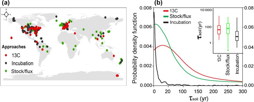
Figure 1. Spatial distributions of observational sites for estimates arated into pool-specific decomposition rates by the decon-
of SOC transit time (τsoil , year). (a) The site locations of measure- volution analysis (Fig. S3a, Liang et al., 2015). We assumed
ments with different approaches. (b) Probability density functions the total soil carbon input equals total soil respiration at the
of τsoil measured with different approaches. Note that the left axis steady state.
is for the 13 C and stock-over-flux approaches, and the right axis is
Based on the theoretical analysis, the dynamics of the
for laboratory incubation studies.
three-pool model can be mathematically described by the
matrix equation (Luo et al., 2003; Xia et al., 2013) as
et al., 2010) and Todd-Brown et al. (2013) (Fig. S1): (1) dC (t)
tropical forest including evergreen broadleaf forest between = I (t) − AKC (t) , (2)
dt
25◦ N and 25◦ S; (2) temperate forest including deciduous
broadleaf, evergreen broadleaf outside of 25◦ N and 25◦ S, where the matrix C(t) = (C1 (t), C2 (t), C3 (t))T is used to
and mixed forest south of 50◦ N; (3) boreal forest includ- describe soil carbon pool sizes. A is a matrix given by
ing evergreen needleleaf forest, deciduous needleleaf forest,
−1 f12 f13
and mixed forest north of 50◦ N; (4) grassland and shrubland A = f21 −1 0 . (3)
including woody savanna south of 50◦ N and savanna and f31 f32 −1
grasslands south of 55◦ N; (5) deserts and savanna including
barren or sparsely vegetated open shrubland south of 55◦ N The elements fij are carbon transfer coefficients, indicating
and closed shrubland south of 50◦ N; (6) tundra; and (7) crop- the fractions of the carbon entering the ith (row) pool from
lands. Other land cover types like permanent wetland, urban, the j th (column) pool. K is a 3×3 diagonal matrix indicating
and bare land were not included in this study. the decomposition rates (the amounts of carbon per unit mass
leaving each of the pools per year). The matrix of K is given
2.2 Outputs of Earth system models from CMIP5 by K = diag (k1 , k2 , k3 ).
The parameters in the three-pool model were estimated
The historical simulation outputs of 12 ESMs participat- based on Bayesian probabilistic inversion (Eq. 4). The pos-
ing in CMIP5 from 1850 to 1860 (https://esgf-data.dkrz.de/ terior probability density function P (θ |Z) of model param-
search/cmip5-dkrz/, last access: 11 January 2016) were ana- eters (θ) can be represented by the prior probability density
lyzed in this study (Table S1). For each model, the SOC, lit- function (P (θ )) and a likelihood function (P (Zlθ )) (Liang
ter C, NPP, and heterotrophic respiration (Rh ) were extracted et al., 2015; Xu et al., 2016). The likelihood function was
from the outputs in historical simulations (cSoil, cLitter, npp, calculated by the minimum error between observed and mod-
and rh, respectively, from the CMIP5 variable list). The litter eled values with Eq. (5). In this study, we adopted the prior
and soil carbon were summed as the bulk soil carbon stock. ranges of model parameters from Liang et al. (2015).
Among the 12 models, only the inmcm4 model did not out-
put NPP, so we calculated it as gross primary production mi- P (θ |Z) ∝ P (Z|θ ) · P (θ ) (4)
nus autotrophic respiration. Due to the diverse spatial resolu-
tions among the models, we aggregated the results of differ- ( )
n
ent models to 1◦ × 1◦ with the nearest interpolation method 1 X X
(Fig. S2). The τsoil of SOC was calculated as the ratio of car- P (Z|θ ) ∝ exp − 2 [Zi (t) − Xi (t) ]2 (5)
2σi (t) i=1 t∈obs(Z)
bon stock over flux (NPP or Rh ):
SOC Here Zi (t) and Xi (t) are the observed and modeled transit
τsoil = . (1) times, and σi2 (t) is the standard deviation of measurements.
flux
The posterior probability density function of the parameters
was constructed with two steps: a proposing step and a mov-
2.3 Estimating the SOC τsoil with a three-pool model ing step. In the first step, the dataset was generated based on
the previously accepted data with a proposal distribution:
To examine whether the major findings of this data–model d(θmax − θmin )
comparison are affected by the one-pool homogenous as- θ new = θ new + , (6)
D
www.biogeosciences.net/16/917/2019/ Biogeosciences, 16, 917–926, 2019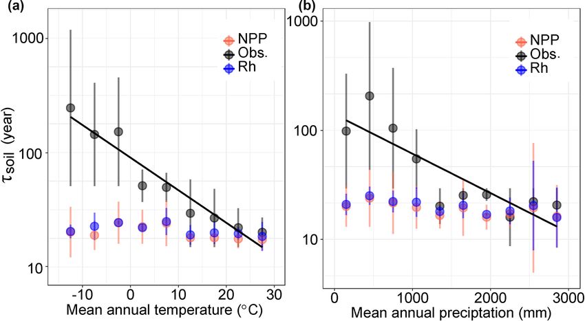
920 J. Wang et al.: Evaluating the simulated mean soil carbon transit times
where θmax and θmin are the maximum and minimum val- oxygen) and vertical transfer process. To understand whether
ues of the given parameters, d is the random variable be- the incorporation of soil vertical profile affects the simula-
tween −0.5 and 0.5 with uniform distribution, and D is used tion of τsoil , we compared the results based on the matrix ap-
to control the proposing step size in this study. In the mov- proach with (i.e., CLM4.5) or without (i.e., CLM4.5_noV)
ing step, the new data θ new is tested against the Metropo- the soil vertical transfer process.
lis criteria to quantify whether it should be accepted or re- In CLM4.5, soil C dynamics was simulated with 10 soil
jected. The parameters of posterior probability density func- layers, and the same organic matter pools among different
tion were constructed with the Metropolis–Hastings algo- vertical soil layers are allowed to mix mainly through diffu-
rithm. The Metropolis–Hastings algorithm was run 50 000 sion and advection. The matrix approach determines the soil
times for observed data. Accepted parameter values were dynamic of each SOC pool by simulating the first-order ki-
used in further analysis. netics as Eq. (9):
Based on the concepts of mean age and mean transit time
published by Rasmussen et al. (2016) and Lu et al. (2018), dC (t)
= B (t) I (t) − Aξ (t) KC (t) V(t)C(t), (9)
the mean carbon age defined as the whole time carbon atoms dt
are stored in the carbon pools and then the mean age of car- where the C(t) is the organic carbon pool size at time t. I(t)
bon a i (t) in a certain carbon pool i could be calculated with is the total organic carbon inputs while B(t) is the vector of
Eq. (7): partitioning coefficients. K is a diagonal matrix that repre-
3
P sents the intrinsic decomposition rate of each carbon pool.
(a j (t) − a i (t)) · fij (t) · Ci − a j (t) · Ii (t) The decomposition rate in the matrix approach is modified
i=1
a i (t) = 1 + , (7) by the transfer matrix A and environmental scalars ξ . The
Ci scalar matrix ξ shown in Eq. (10) is the environmental factor
where the fij (t) values are the carbon fraction transfer coef- to modify the SOC intrinsic decomposition rate. Each scalar
ficients from j th to ith pools, and Ii (t) is the external input matrix combines temperature (ξT ), water (ξW ), oxygen (ξO ),
into the ith carbon pool. The transit time τi (t) was defined depth (ξD ), and nitrogen (ξN ) controlled scalars for SOC de-
as the mean age of carbon atoms leaving the carbon pool at a cay.
specific time:
ξ 0 = ξT ξW ξO ξD ξN (10)
d
X
τi (t) = fi (t) · ai (t) , (8) A is the horizontal carbon transfer matrix, which quantifies
i=1 C movement among different carbon pools shown as matrix
where the fi (t) is the fraction of carbon with mean age ai (t). (10). The non-diagonal entries Aij shown in matrix (10) rep-
resent the fraction of carbon that moves from the j th to the
2.4 Matrix approach through CLM4.5 and ith pools. In CLM4.5 and CLM4.5_noV, transfer coefficients
CLM4.5_noV are the same in each soil layer.
The Community Land Model version 4.5 (CLM4.5) is the 0 0 0 0 0 0 0
terrestrial component of the Community Earth System Model 0 0 0 0 0 0 0
(CESM). This version mainly consists of exchanges among 0 0 0 0 0 0 0
different carbon and nitrogen pools and other biogeochem- A= 0 0 0 f44 0 0 0
(11)
ical cycles and includes a vertical dimension of soil carbon 0 f52 f53 0 f55 f56 f57
and nitrogen transformations (Koven et al., 2013). The ma- 0 0 0 f64 f65 f66 0
trix approach was applied to extract the soil module from 0 0 0 0 f75 f76 f77
the original CLM4.5, which could evaluate which processes
influence τsoil in the model (Huang et al., 2017). Once we V(t) is the vertical carbon transfer coefficient matrix among
obtain the total carbon pool and Rh in each pool, we can cal- different soil layers, and each of the diagonal blocks is a tridi-
culate the τsoil with Eq. (1). We represented the structure of agonal matrix that describes transfer coefficients with Vij (t).
SOC as seven carbon pools as (i) one coarse woody debris In this section, CLM4.5_noV assumes no vertical transfers
(CWD) pool, (ii) three litter pools (litter1, litter2, and litter3), in all pools. Therefore, V(t) for CLM4.5_noV is a blank ma-
and (iii) three soil carbon pools (soil1, soil2, and soil3). In trix in the simulation. In contrast, CLM4.5 was assigned by
this matrix, carbon is transferred from three litter pools and a matrix with vertical transfers in each C pool. The vertical
CWD to three soil pools with different transfer rates. In each transfer rates among different C pool categories in CLM4.5
layer, these transfer rates are regulated by the transfer coef- are matrix (12).
ficients and fractions. C inputs from litterfall were allocated
into different C compartments by modifications by soil envi-
ronmental factors (temperature, moisture, nitrogen, and soil
Biogeosciences, 16, 917–926, 2019 www.biogeosciences.net/16/917/2019/J. Wang et al.: Evaluating the simulated mean soil carbon transit times 921
studies. Thus, the τsoil values from the laboratory incubation
studies were excluded in the following analyses.
V(t) = (12) We then integrated the estimates of τsoil based on the 13 C
0 0 0 0 0 0 0 and stock-over-flux approaches to examine the inter-biome
0 V22 (t) 0 0 0 0 0 difference. As shown by Fig. 2b, the longest τsoil was found
0 0 V33 (t) 0 0 0 0
0
0 0 V44 (t) 0 0 0 in desert and shrubland (170; 58 to 508) and tundra (159;
0
0 0 0 V55 (t) 0 0 39 to 649 years). Boreal forest (58; 25 to 170 years) has a
0 0 0 0 0 V66 (t) 0 longer τsoil than the temperate (44; 13 to 89 years) and trop-
0 0 0 0 0 0 V77 (t) ical forests (15; 9 to 130 years). Grassland and savanna had
2.5 Statistical analyses short τsoil (35; 21 to 57 years) and croplands had moderate
(62; 21 to 120 years) τsoil in comparison with other biomes
The median and interquartile were used for the quantifica- (Fig. 2).
tion of both observational and modeling results due to the
fact that the probability distribution of τsoil is not normal. To 3.2 Modeled τsoil in the CMIP5 ensemble and its
test the difference in τsoil among three approaches, we first estimation biases
normalized the data with the log-transformation and then ap-
plied the one-way ANOVA with a multi-comparison tech- The longest ensemble mean τsoil values of multiple mod-
nique (Fig. 1b insert). The linear regression and correlation els were found in dry and cold regions (Fig. 2). In com-
analyses were performed in R (3.2.1; R development Core parison with the integrated observations from 13 C and stock
team, 2015). over flux, the modeled τsoil values were significantly shorter
The Gaussian kernel density estimation was used to obtain across all biomes (Fig. 2b insert). The negative bias was
the distributions of observed transit times (Sheather and Mar- larger in dry (desert, grassland, and savanna) and cold (tun-
ron, 1990; Saoudi et al., 1997). The Gaussian kernel density dra and boreal forest) regions than tropical and temperate
estimation is a nonparametric approach to estimate the prob- forests. The longest modeled τsoil appeared in the tundra
ability density function of a random variable. Let (x1 x2 · · ·, ecosystem with a median of 64 years. The modeled median
xn ) denote the observed SOC τsoil with density function f as τsoil values were also shorter than observations in tropical
below: forest (9 years), temperate forests (13 years), boreal forest
n (24 years), grassland/savanna (25 years), desert and shrub-
1 X x − xi land (58 years), and croplands (27 years) (Fig. 2). In compar-
fˆh (x) = K( ), (13)
nh i=1 h ison with the observations, the models obviously underesti-
mated the τsoil in the cold and dry biomes (Fig. 2b). A recent
where K is the nonnegative function than integrates to one global data–model comparison study at 0.5◦ ×0.5◦ resolution
and has a mean of zero, and h>0 is a smoothing parameter also detected a similar spatial pattern of underestimation bias
called the bandwidth. The bandwidth for approaches of sta- in ecosystem C turnover time (Carvalhais et al., 2014), but its
ble isotope 13 C, stock over flux, and incubation are 48.61, magnitudes of bias in the cold regions are much smaller than
35.13, and 2.62, respectively. those found in this study.
By grouping the τsoil into different climatic categories,
3 Results and discussion we found that the observed τsoil significantly covaried with
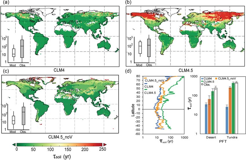
MAT (y = −5.28x + 156.04, r 2 = 0.48, P922 J. Wang et al.: Evaluating the simulated mean soil carbon transit times
Figure 2. Global spatial variation of SOC transit time (τsoil ) with climate and the difference of τsoil estimation between observations and
models. (a) Spatial variation of τsoil with mean annual temperature (MAT) and mean annual precipitation (MAP). (b) Comparisons of
modeled against observed τsoil . Details for the classification of biomes are provided in the method section.
Figure 4. The SOC transit time (τsoil ) calculated from the one- and
three-pool models under the steady-state assumption.
Figure 3. Relationships between SOC transit time (τsoil ) and cli-
mate factors in both observations and CIMP5 models. The black
solid lines show the negative correlation between τsoil and (a) mean
annual temperature and (b) mean annual precipitation. The black model structures showed the largest underestimation of τsoil
dots indicate the aggregated τsoil over each category of MAT (y = in the tundra and desert (Fig. 4).
−5.47x + 1971.5, r 2 = 0.49, PJ. Wang et al.: Evaluating the simulated mean soil carbon transit times 923 Figure 5. Simulated SOC transit time (τsoil ) by CLM4 (a, median global τsoil = 20.56 years), CLM4.5 (b, median global τsoil = 127.50 years), and CLM4.5_noV (c, median global τsoil = 22.24 years). Panel (d) shows the latitudinal spatial distribution of the mean τsoil of different models in desert and tundra. The inserts in (a)–(c) compare the τsoil between models and observations. The bottom and top of the box represent the first and third quartiles. ments with a matrix approach (i.e., there is no vertical C affect the estimation of τsoil but are so far fully considered by transfer; thus, the vertical matrix is a zero matrix in Eq. 12), the CMIP5 models (Luo et al., 2016). For example, adding we showed a similar pattern of underestimation on τsoil by soil microbial dynamics could increase τsoil in cold regions CLM4.5 (i.e., CLM4.5_noV in Fig. 5). Huang et al. (2017) by lowering the transfer proportion of decomposed SOC to also reported the longer τsoil and high carbon storage capac- the atmosphere (Wieder et al., 2013). By contrast, the incor- ity in northern high latitudes. These results suggest that the poration of nitrogen cycles might shorten τsoil by increasing vertically resolved soil biogeochemistry is promising in im- plant C transfers to short-lived litter pools (e.g., O-CN and proving the τsoil estimates by ESMs. However, it should be CABLE models) (Gerber et al., 2010) or reducing litter C noted that the spatial variation of τsoil is still largely underes- transfers to the slow soil C pools (e.g., LM3V model) (Xia et timated by the CLM4.5 (Fig. 5b insert). al., 2013). Higher NPP values simulated by ESMs in the cold and Large challenges still exist in using observations derived dry regions have been reported by previous studies (Shao et from different methods to constrain the modeled τsoil . Labo- al., 2013; Smith et al., 2016; Xia et al., 2017). The models ratory incubation studies report much shorter τsoil than other produce high NPP in cold regions largely because they over- methods, mainly due to the optimized soil moisture and/or estimate the efficiency of plants transferring assimilated C to temperature during the soil incubation (Stewart et al., 2008; growth (Xia et al., 2017). The CMIP5 models overestimate Feng et al., 2016). This suggests that the ESM models will the precipitation and underestimate the dryland expansion 4- largely underestimate τsoil if its turnover parameters are de- fold during 1996–2005 (Ji et al., 2015), which could lead to rived from laboratory incubation studies. It should be noted high NPP and fast SOC turnover rates. These results suggest that the observations from the 13 C and the stock-over-flux that once the NPP simulation is improved without the cor- approaches in this study are derived for the bulk soil. How- rection of the τsoil underestimation, the models will produce ever, SOC is commonly represented as multiple pools with smaller SOC stock in the cold and dry ecosystems. different cycling rates in most of the CMIP5 models (Luo This study shows that adding the vertical resolved biogeo- et al., 2016; Sierra et al., 2017, 2018; Metzler and Sierra, chemistry is a promising approach to correct the bias of τsoil 2018). As synthesized by Sierra et al. (2017), the observa- in current models. However, other processes such as micro- tions of τsoil are useful for a specific model once its pool bial dynamics, SOC stabilization, and nutrient cycles could structure is identified. This study also detects a difference www.biogeosciences.net/16/917/2019/ Biogeosciences, 16, 917–926, 2019
924                                                    J. Wang et al.: Evaluating the simulated mean soil carbon transit times

in the estimated τsoil between the one- and three-pool mod-           Acknowledgements. We appreciate the anonymous reviewers for
els (Fig. 4). Thus, model databases, such as bgc-md (https:           their valuable suggestions. We also appreciate Katherine Todd-
//github.com/MPIBGC-TEE/bgc-md, last access: 2 February               Brown for her support of the soil data in CMIP5 and Deli Zhai for
2019), are a useful tool to improve the integration of obser-         valuable comments. The model simulations analyzed in this study
vations and soil C models. An enhanced transparency of C-             were obtained from the Earth System Grid Federation CMIP5
                                                                      online portal hosted by the Program for Climate Model Diagnosis
cycle model structure in ESMs is highly recommended, es-
                                                                      and Intercomparison at Lawrence Livermore National Laboratory
pecially when they participate in the future model intercom-          (https://esgf-node.llnl.gov/projects/esgf-llnl/, last access: 4 Octo-
parison projects such as CMIP6 (Jones et al., 2016).                  ber 2018). This work was financially supported by the National
                                                                      Natural Science Foundation (31722009, 31800400, 41630528), the
                                                                      National Key R&D Program of China (2017YFA0604603), the
4   Conclusions
                                                                      Fok Ying Tong Education Foundation for Young Teachers in the
                                                                      Higher Education Institutions of China (grant no. 161016), and the
This study detected large underestimation biases of τsoil in
                                                                      National 1000 Young Talents Program of China.
ESMs in cold and dry biomes, especially the tundra and
desert. Improving the modeling of SOC dynamics in these               Edited by: Jens-Arne Subke
regions is important because the cold ecosystems (e.g., the           Reviewed by: two anonymous referees
permafrost regions) are critical for global C feedback to fu-
ture climate change (Schuur et al., 2015) and the dry regions
strongly regulate the interannual variability of land CO2 sink
(Poulter et al., 2014; Ahlström et al., 2015). The current gen-       References
eration of ESMs represents the soil C processes with a similar
                                                                      Ahlström, A., Raupach, M. R., Schurgers, G., Smith, B., Arneth, A.,
model formulation as first-order C transfers among multiple
                                                                        Jung, M., Reichstein, M., Canadell, J. G., Friedlingstein, P., Jain,
pools (Sierra and Markus, 2015; Luo et al., 2016; Metzler               A. K., and Kato, E.: The dominant role of semi-arid ecosystems
and Sierra, 2018). Thus, tremendous research efforts are still          in the trend and variability of the land CO2 sink, Science, 348,
required to attribute the underestimation biases of τsoil in cur-       895–899, https://doi.org/10.1126/science.aaa1668, 2015.
rent ESMs to their sources, such as model structure, parame-          Allison, S. D., Matthew, D. W., and Mark, A. B.: Soil-carbon
terization, and climate forcing. Reducing these biases would            response to warming dependent on microbial physiology, Nat.
largely improve the accuracy of ESMs in the projection of the           Geosci., 3, 336–340, https://doi.org/10.1038/ngeo846, 2010.
future terrestrial C cycle and its feedback to climate change.        Balesdent, J., Mariotti, A., and Guillet, B.: Natural 13 C abun-
Recent modeling activities aiming to increase the soil hetero-          dance as a tracer for studies of soil organic matter dynamics,
geneity, for example, soil vertical profile (Koven et al., 2013,        Soil Biol. Biochem., 19, 25–30, https://doi.org/10.1016/0038-
2017) and microbial dynamics (Allison et al., 2010; Wieder              0717(87)90120-9, 1987.
                                                                      Bernstein, L., Bosch, P., Canziani, O., Chen, Z., Christ, R., and Ri-
et al., 2013), are promising. Overall, this study shows the
                                                                        ahi, K.: IPCC, 2007: Climate Change 2007: Synthesis Report,
great spatial variation of τsoil in natural ecosystems, and we          2008.
recommend more research efforts to improve its representa-            Bloom, A. A., Exbrayat, J. F., van der Velde, I. R., Feng, L.,
tion by ESMs in the future.                                             and Williams, M.: The decadal state of the terrestrial carbon
                                                                        cycle: Global retrievals of terrestrial carbon allocation, pools,
                                                                        and residence times, P. Natl. Acad. Sci. USA, 113, 1285–1290,
Data availability. The data are available from the corresponding        https://doi.org/10.1073/pnas.1515160113, 2016.
author by request.                                                    Bolin, B. and Henning, R.: A note on the concepts of age distri-
                                                                        bution and transit time in natural reservoirs. Tellus, 25, 58–62,
                                                                        https://doi.org/10.1111/j.2153-3490.1973.tb01594.x, 1973.
Supplement. The supplement related to this article is available       Bolker, B. M., Pacala, S. W., and Parton Jr., W. J.: Linear analysis of
online at: https://doi.org/10.5194/bg-16-917-2019-supplement.           soil decomposition: insights from the century model, Ecol. Appl.,
                                                                        8, 425–439, 1998.
                                                                      Bradford, M. A., Wieder, W. R., Bonan, G. B., Fierer, N., Raymond,
Author contributions. JX designed the study. JW collected and or-       P. A., and Crowther, T. W.: Managing uncertainty in soil carbon
ganized the data. LJ provided the CMIP5 and HWSD data. XX pro-          feedbacks to climate change, Nat. Clim. Change, 6, 751–758,
vided the laboratory incubation data. YH provided the CLM4.5 ma-        https://doi.org/10.1038/nclimate3071, 2016.
trix module. JW and JX wrote the first draft, and all other authors   Carvalhais, N., Forkel, M., Khomik, M., Bellarby, J., Jung, M.,
contributed to revision and discussion of the results.                  Migliavacca, M., Mu, M., Saatchi, S., Santoro, M., Thurner,
                                                                        M., and Weber, U.: Global covariation of carbon turnover times
                                                                        with climate in terrestrial ecosystems, Nature, 514, 213–217,
                                                                        https://doi.org/10.1038/nature13731, 2014.
Competing interests. The authors declare that they have no conflict
                                                                      Ciais, P., Sabine, C., Bala, G., Bopp, L., Brovkin, J., and Thornton,
of interest.
                                                                        P.: Climate Change 2013: the physical science basis. Contribu-
                                                                        tion of Working Group I to the Fifth Assessment Report of the

Biogeosciences, 16, 917–926, 2019                                                             www.biogeosciences.net/16/917/2019/
J. Wang et al.: Evaluating the simulated mean soil carbon transit times 925
Intergovernmental Panel on Climate Change, edited by: Stocker, Biogeosciences, 10, 7109–7131, https://doi.org/10.5194/bg-10-
T. F., Qin, D., Plattner, G. K., Tignor, M., Allen, S. K, Boschung, 7109-2013, 2013.
J., Nauels, A., Xia, Y., Bex, V., and Midgley, P. M., Cambridge Koven, C. D., Hugelius, G., Lawrence, D. M., and Wieder, W.
Univ. Press, 465–570, 2013. R.: Higher climatological temperature sensitivity of soil carbon
FAO/IIASA/ISRIC/ISSCAS/JRC, Harmonized World Soil in cold than warm climates, Nat. Clim. Change, 7, 817–822,
Database (version 1.10), FAO, Rome, Italy and IIASA, https://doi.org/10.1038/nclimate3421, 2017.
Laxenburg, Austria, 2012. Liang, J., Li, D., Shi, Z., Tiedje, J. M., Zhou, J., Schuur, E. A. G.,
Feng, W., Shi, Z., Jiang, J., Xia, J., Liang, J., Zhou, J., and Luo, Konstantinidis, K. T., and Luo, Y.: Methods for estimating tem-
Y.: Methodological uncertainty in estimating carbon turnover perature sensitivity of soil organic matter based on incubation
times of soil fractions, Soil Biol. Biochem., 100, 118–124, data: A comparative evaluation, Soil Biol. Biochem., 80, 127–
https://doi.org/10.1016/j.soilbio.2016.06.003, 2016. 135, https://doi.org/10.1016/j.soilbio.2014.10.005, 2015.
Friedl, M. A., Sulla-Menashe, D., Tan, B., Schneider, A., Ra- Lu, X., Wang, Y.-P., Luo, Y., and Jiang, L.: Ecosystem carbon tran-
mankutty, N., Sibley, A., and Huang, X.: MODIS Collection sit versus turnover times in response to climate warming and ris-
5 global land cover: Algorithm refinements and characteriza- ing atmospheric CO2 concentration, Biogeosciences, 15, 6559–
tion of new datasets, Remote Sens. Environ., 114, 168–182, 6572, https://doi.org/10.5194/bg-15-6559-2018, 2018.
https://doi.org/10.1016/j.rse.2009.08.016, 2010. Luo, Y., White, L. W., Canadell, J. G., DeLucia, E. H., Ellsworth,
Friedlingstein, P., Cox, P., Betts, R., Bopp, L., von Bloh, W., D. S., Finzi, A., Lichter, J., and Schlesinger, W. H.: Sustainability
Brovkin, V., Cadule, P., Doney, S., Eby, M., Fung, I., and of terrestrial carbon sequestration: A case study in Duke Forest
Bala, G.: Climate-carbon cycle feedback analysis: Results from with inversion approach, Global Biogeochem. Cy., 17, 12101–
the C4MIP model intercomparison, J. Clim., 19, 3337–3353, 2113, https://doi.org/10.1029/2002GB001923, 2003.
https://doi.org/10.1175/JCLI3800.1, 2006. Luo, Y., Ahlström, A., Allison, S. D., Batjes, N. H., Brovkin, V.,
Fröberg, M., Tipping, E., Stendahl, J., Clarke, N., and Bryant, Carvalhais, N., Chappell, A., Ciais, P., Davidson, E. A., Finzi,
C.: Mean residence time of O horizon carbon along a cli- A., and Georgiou, K.: Toward more realistic projections of soil
matic gradient in Scandinavia estimated by 14 C measure- carbon dynamics by Earth system models, Glob. Biogeochem.
ments of archived soils, Biogeochemistry, 104, 227–236, Cy., 30, 40–56, https://doi.org/10.1002/2015GB005239, 2016.
https://doi.org/10.1007/s10533-010-9497-3, 2011. Metzler, H. and Sierra, C. A.: Linear autonomous compartmental
Gerber, S., Hedin, L. O., Oppenheimer, M., Pacala, S. W., and models as continuous-time Markov chains: transit-time and age
Shevliakova, E.: Nitrogen cycling and feedbacks in a global distributions, Math. Geosci., 50, 1–34, 2018.
dynamic land model, Global Biogeochem. Cy., 24, GB1001, Metzler, H., Müller, M., and Sierra, C. A.: Transit-time and
https://doi.org/10.1029/2008GB003336, 2010. age distributions for nonlinear time-dependent compartmen-
He, Y., Trumbore, S. E., Torn, M. S., Harden, J. W., Vaughn, L. J., tal systems, P. Natl. Acad. Sci. USA, 22, 201705296,
Allison, S. D., and Randerson, J. T.: Radiocarbon constraints im- https://doi.org/10.1073/pnas.1705296115, 2018.
ply reduced carbon uptake by soils during the 21st century, Sci- Mishra, U., Drewniak, B., Jastrow, J. D., Matamala, R. M.,
ence, 353, 1419–1424, https://doi.org/10.1126/science.aad4273, and Vitharana, U. W. A.: Spatial representation of or-
2016. ganic carbon and active-layer thickness of high latitude soils
Huang, Y., Lu, X., Shi, Z., Lawrence, D., Koven, C.D., in CMIP5 earth system models, Geoderma, 300, 55–63,
Xia, J., Du, Z., Kluzek, E., and Luo, Y.: Matrix approach https://doi.org/10.1016/j.geoderma.2016.04.017, 2017.
to land carbon cycle modeling: A case study with Com- NASA LP DAAC Land Cover Type Yearly L3 Global 0.05 Deg
munity Land Model, Glob. Change Biol., 24, 1394–1404, CMG (MCD12C1), USGS/Earth Resources Observation and
https://doi.org/10.1111/gcb.13948, 2017. Science (EROS) Center, Sioux Falls, South Dakota, available at:
Hutchinson, M. F. and Xu, T.: Anusplin version 4.2 user guide. Cen- https://lpdaac.usgs.gov/products/modisproductstable/landcover/
tre for Resource and Environmental Studies, The Australian Na- yearlyl3global0.05degcmg/mcd12c1 (last access: 14 April
tional University, Canberra, 54, 2004. 2014), 2008.
Ji, M., Huang, J., Xie, Y., and Liu, J.: Comparison of dryland cli- Parry, M., Parry, M. L., Canziani, O., Palutikof, J., Van der Linden,
mate change in observations and CMIP5 simulations, Adv. At- P., and Hanson, C.: Climate Change 2007: Impacts, Adaptation
mos. Sci., 32, 1565–1574, https://doi.org/10.1007/s00376-015- and Vulnerability, Assessment Report of the Intergovernmental
4267-8, 2015. Panel on Climate Change, Cambridge Univ. Press, Cambridge,
Jones, C. D., Arora, V., Friedlingstein, P., Bopp, L., Brovkin, V., UK, 211–272, 2007.
Dunne, J., Graven, H., Hoffman, F., Ilyina, T., John, J. G., Poulter, B., Frank, D., Ciais, P., Myneni, R. B., Andela, N., Bi,
Jung, M., Kawamiya, M., Koven, C., Pongratz, J., Raddatz, J., Broquet, G., Canadell, J. G., Chevallier, F., Liu, Y. Y., and
T., Randerson, J. T., and Zaehle, S.: C4MIP – The Coupled Running, S. W.: Contribution of semi-arid ecosystems to interan-
Climate-Carbon Cycle Model Intercomparison Project: experi- nual variability of the global carbon cycle, Nature, 509, 600–603,
mental protocol for CMIP6, Geosci. Model Dev., 9, 2853–2880, https://doi.org/10.1038/nature13376, 2014.
https://doi.org/10.5194/gmd-9-2853-2016, 2016. Rasmussen, M., Hastings, A., Smith, M. J., Agusto, F. B., Chen-
Koven, C. D., Riley, W. J., Subin, Z. M., Tang, J. Y., Torn, M. Charpentier, B. M., Hoffman, F. M., Jiang, J., Todd-Brown, K. E.,
S., Collins, W. D., Bonan, G. B., Lawrence, D. M., and Swen- Wang, Y., Wang, Y. P., and Luo, Y.: Transit times and mean ages
son, S. C.: The effect of vertically resolved soil biogeochemistry for nonautonomous and autonomous compartmental systems,
and alternate soil C and N models on C dynamics of CLM4, J. Math. Biol., 73, 1379–1398, https://doi.org/10.1007/s00285-
016-0990-8, 2016.
www.biogeosciences.net/16/917/2019/ Biogeosciences, 16, 917–926, 2019926 J. Wang et al.: Evaluating the simulated mean soil carbon transit times Sanderman, J. Ronald, G. A., and Dennis, D. B.: Application of Stewart, C. E., Paustian, K., Conant, R. T., Plante, A. F., and eddy covariance measurements to the temperature dependence of Six, J.: Soil carbon saturation: evaluation and corroboration soil organic matter mean residence time, Glob. Biogeochem. Cy., by long-term incubations, Soil Biol. Biochem., 40, 1741–1750, 17, 301–3015, https://doi.org/10.1029/2001GB001833, 2003. https://doi.org/10.1016/j.soilbio.2008.02.014, 2008. Saoudi, S., Ghorbel, F., and Hillion, A.: Some statistical properties Todd-Brown, K. E. O., Randerson, J. T., Post, W. M., Hoffman, F. of the kernel – diffeomorphism estimator, Appl. Stoch. Model M., Tarnocai, C., Schuur, E. A. G., and Allison, S. D.: Causes Data Anal., 13, 39–58, https://doi.org/10.1002/(SICI)1099- of variation in soil carbon simulations from CMIP5 Earth system 0747(199703)13:13.0.CO;2-J, 1997. models and comparison with observations, Biogeosciences, 10, Schmidt, M. W., Torn, M. S., Abiven, S., Dittmar, T., Guggenberger, 1717–1736, https://doi.org/10.5194/bg-10-1717-2013, 2013. G., Janssens, I. A., Kleber, M., Kögel-Knabner, I., Lehmann, Trumbore, S. E.: Comparison of carbon dynamics in tropical and J., Manning, D. A., and Nannipieri, P.: Persistence of soil or- temperate soils using radiocarbon measurements, Glob. Bio- ganic matter as an ecosystem property, Nature, 478, 49–56, geochem. Cy., 7, 275–290, https://doi.org/10.1029/93GB00468, https://doi.org/10.1038/nature10386, 2011. 1993. Schuur, E. A. G., McGuire, A. D., Schädel, C., Grosse, G., Trumbore, S. E., Chadwick, O. A., and Amundson, R.: Rapid Harden, J. W., Hayes, D. J., Hugelius, G., Koven, C. D., exchange between soil carbon and atmospheric carbon diox- Kuhry, P., Lawrence, D. M., and Natali, S. M.: Climate change ide driven by temperature change, Science, 272, 393–396, and the permafrost carbon feedback, Nature, 520, 171–179, https://doi.org/10.1126/science.272.5260.393, 1996. https://doi.org/10.1038/nature14338, 2015. Wieder, W. R., Bonan, G. B., and Allison, S. D.: Global Shao, P., Zeng, X., Sakaguchi, K., Monson, R. K., and soil carbon projections are improved by modelling mi- Zeng, X.: Terrestrial carbon cycle: climate relations in eight crobial processes, Nat. Clim. Change, 3, 909–912, CMIP5 earth system models, J. Clim., 26, 8744–8764, https://doi.org/10.1038/nclimate1951, 2013. https://doi.org/10.1175/JCLI-D-12-00831.1, 2013. Xia, J., Luo, Y., Wang, Y. P., and Hararuk, O.: Traceable Sheather, S. J. and Marron, J. S.: Kernel quan- components of terrestrial carbon storage capacity in bio- tile estimators, J. Am. Stat. Assoc., 85, 410–416, geochemical models, Glob. Change Biol., 19, 2104–2116, https://doi.org/10.1080/01621459.1990.10476214, 1990. https://doi.org/10.1111/gcb.12172, 2013. Sierra, C. A. and Markus, M.: A general mathematical framework Xia, J., McGuire, A. D., Lawrence, D., Burke, E., Chen, G., for representing soil organic matter dynamics, Ecol. Monogr., 85, Chen, X., Delire, C., Koven, C., MacDougall, A., Peng, S., and 505–524, https://doi.org/10.1890/15-0361.1, 2015. Rinke, A.: Terrestrial ecosystem model performance in simulat- Sierra, C. A., Müller, M., Metzler, H., Manzoni, S., and Trum- ing productivity and its vulnerability to climate change in the bore, S. E.: The muddle of ages, turnover, transit, and residence northern permafrost region, J. Geophys. Res., 122, 430–446, times in the carbon cycle, Glob. Change Biol., 23, 1763–1773, https://doi.org/10.1002/2016JG003384, 2017. https://doi.org/10.1111/gcb.13556, 2017. Xu, X., Shi, Z., Li, D., Rey, A., Ruan, H., Craine, J. M., Sierra, C. A., Ceballos-Núñez, V., Metzler, H., and Müler, M.: Rep- Liang, J., Zhou, J., and Luo, Y.: Soil properties con- resenting and understanding the carbon cycle using the theory of trol decomposition of soil organic carbon: results from compartmental dynamical systems, J. Adv. Model. Earth Sy., 10, dataassimilation analysis, Geoderma, 262, 235–242, 1729–1734, https://doi.org/10.1029/2018MS001360, 2018. https://doi.org/10.1016/j.geoderma.2015.08.038, 2016. Six, J. and Jastrow, J. D.: Organic matter turnover, Encycl. of Soil Zhang, K., Dang, H., Zhang, Q., and Cheng, X.: Soil carbon dynam- Science, 2002, 936–942, 2002. ics following landuse change varied with temperature and precip- Smith, W. K., Reed, S. C., Cleveland, C. C., Ballantyne, A. P., An- itation gradients: evidence from stable isotopes, Glob. Change deregg, W. R., Wieder, W. R., Liu, Y. Y., and Running, S. W.: Biol., 21, 2762–2772, https://doi.org/10.1111/gcb.12886, 2015. Large divergence of satellite and Earth system model estimates of global terrestrial CO2 fertilization, Nat. Clim. Change, 6, 306– 310, https://doi.org/10.1038/nclimate2879, 2016. Spohn, M. and Sierra, C. A.: How long do elements cy- cle in terrestrial ecosystems?, Biogeochemistry, 139, 69–83, https://doi.org/10.1007/s10533-018-0452-z, 2018. Biogeosciences, 16, 917–926, 2019 www.biogeosciences.net/16/917/2019/
You can also read