Evaluation of Biogas Potential from Livestock Manures and Multicriteria Site Selection for Centralized Anaerobic Digester Systems: The Case of ...
←
→
Page content transcription
If your browser does not render page correctly, please read the page content below
sustainability

Article
Evaluation of Biogas Potential from Livestock
Manures and Multicriteria Site Selection for
Centralized Anaerobic Digester Systems:
The Case of Jalisco, México
Diego Díaz-Vázquez 1 , Susan Caroline Alvarado-Cummings 1 , Demetrio Meza-Rodríguez 2 ,
Carolina Senés-Guerrero 1 , José de Anda 3, * and Misael Sebastián Gradilla-Hernández 1, *
 1    Tecnologico de Monterrey, Escuela de Ingenieria y Ciencias, Av. General Ramón Corona 2514,
      Nuevo México, Zapopan CP 45138, Mexico; A01229693@itesm.mx (D.D.-V.);
      susancaroline.ac@gmail.com (S.C.A.-C.); carolina.senes@tec.mx (C.S.-G.)
 2    Departamento de Ecologia y Recursos Naturales, Universidad de Guadalajara, Independencia Nacional
      #151, Autlan de Navarro CP 48900, Mexico; demetrio.meza@academicos.udg.mx
 3    Centro de Investigación y Asistencia en Tecnología y Diseño del Estado de Jalisco, A. C. Normalistas 800,
      Guadalajara CP 44270, Mexico
 *    Correspondence: janda@ciatej.mx (J.d.A.); msgradilla@tec.mx (M.S.G.-H.);
      Tel.: +52-(33)-33455200 (J.d.A.); +52-(33)-36693000 (M.S.G.-H.)

 Received: 14 March 2020; Accepted: 14 April 2020; Published: 26 April 2020

 Abstract: The state of Jalisco is the largest livestock producer in Mexico, leading in the production
 of swine, eggs, and milk. This immense production generates enormous amounts of waste as
 a byproduct of the process itself. The poor management of livestock-derived waste can lead to
 multiple environmental problems like nutrient accumulation in soil, water eutrophication, and air
 pollution. The aim of this work is to establish a replicable geographic information system (GIS)-based
 methodology for selecting priority sites in which to implement anaerobic digestion units. These
 units will use multiple parameters that evaluate environmental risks and viability factors for the
 units themselves. A weighted overlay analysis was used to identify critical regions and, based on
 the results, clusters of individual livestock production units (LPUs) across the state were selected.
 Nitrogen and phosphorus recovery, as well as the energetic potential of the selected clusters, were
 calculated. Four clusters located mainly in the Los Altos region of Jalisco were selected as critical and
 analyzed. The results indicate that Jalisco has the potential to generate 5.5% of its total electricity
 demand if the entirety of its livestock waste is treated and utilized in centralized anaerobic digestion
 units. Additionally, 49.2 and 31.2 Gg of nitrogen and phosphorus respectively could be valorized,
 and there would be an estimated total reduction of 3012.6 Gg of carbon dioxide equivalent (CO2 eq).

 Keywords: GIS-based methodology; livestock manure; anaerobic digestion; energy production;
 spatial analysis; waste valorization

1. Introduction

1.1. Livestock Waste Management
     The poor management of livestock waste contributes to environmental problems. The main
environmental concerns regarding livestock manure can be divided into three categories: accumulation
of nutrients in soil, water eutrophication, and air pollution caused by greenhouse gases [1]. Nutrient
accumulation in soil can lead to uncontrolled amounts of nitrogen and phosphorus, which can harbor
a wide variety of microorganisms that can be pathogenic [2]. Moreover, the animal manure and

Sustainability 2020, 12, 3527; doi:10.3390/su12093527                         www.mdpi.com/journal/sustainability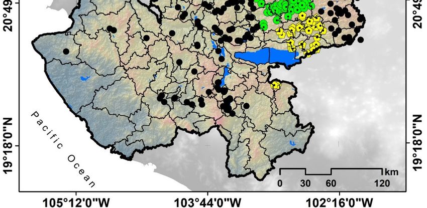
Sustainability 2020, 12, 3527                                                                        2 of 32

wastewater generated by a livestock producing unit (LPU) have high concentrations of metals (such
as copper, zinc, arsenic, and cadmium), mainly due to the mineral components of livestock feed
that are excreted in manure and to the corrosion of the metallic elements in animal enclosures [3,4].
The long-term application of untreated manure to soil can lead to leaching and accumulation in
groundwater and water bodies. This in turn can cause increased phytotoxicity, reduced soil fertility
and productivity, and toxicity of crops and food products grown on the contaminated soil [5,6].
       The transfer of excessive amounts of nutrients and effluents (e.g., slurry, feces, and urine) caused
by surface runoff and/or leaching in livestock feeding areas significantly contributes to water quality
degradation and eutrophication [7]. Air can be polluted by the emission of greenhouse gases (GHGs)
such as methane, nitrous oxide, and ammonia, [8] which contribute to global warming. Unmanaged
agricultural and livestock waste may have adverse effects on public health [3,9] due to odors, excessive
levels of phosphorus and nitrogen on surface and groundwater, and their potential to spread human
pathogens [10]. Further, the ingestion of nitrate and phosphate compounds can lead to diseases such
as hypertension, gastrointestinal illness, birth defects, and even infant mortality [11,12].
       To decrease the environmental impact of livestock manure various processing technologies have
been developed. Composting is widely used because of its cost efficiency [13], though it has been
argued that when used as the sole management strategy for these wastes it causes other environmental
problems due to the resulting emissions and leachates, which negatively impact air, soil, and water
quality [14]. However, there are relatively simple practices that can help prevent leaching, such as
increasing compost water holding capacity by adding various bulking agents, protecting the compost
from rainfall, and impermeabilizing the composting area correctly [14]. Additionally, composting
plants may be equipped with leachate recirculators to ensure that the liquid component generated
during the degradation process is integrated back into the process matrix, thus increasing nutrient
distribution and pH buffering [15]. Unfortunately, most of the composting done by micro and small
producers in Jalisco is carried out in low technification conditions [16].
       There are other techniques for manure treatment such as anaerobic digestion (AD), biological
treatment, incineration, pyrolysis, and gasification [14,17–19], which are not as commonly used
because of their costs, time investment required, and/or ineffectiveness [20]. For instance, AD presents
numerous advantages such as pollution reduction (when considering GHG emissions and nutrient
leachates), production of valuable byproducts such as fertilizers, and the production of renewable
energy. However, AD is expensive, time-consuming, requires high land use, and great volumes of
biomass (which is usually gathered by collecting waste from multiple sites) [21,22]. Biological treatment
by aerobic digestion is the biochemical oxidative stabilization of wastewater sludge. It can reduce GHG
emissions, odors, and pathogens; however, it entails higher capital costs for aeration and monitoring,
and it does not produce useful byproducts such as methane [23]. Thermal conversion techniques, such
as gasification and pyrolysis, have been widely used to convert organic waste into energy. The main
drawback of these treatment methods is that they require a partially dried substrate in order to achieve
positive energy recovery rates [24]. Since manure and livestock wastewater have a high moisture
content, the required drying process could lead to an energy deficit in the thermal conversion process,
thus making manure less economically advantageous when compared to other treatment methods,
and therefore unsuitable for managing large volumes of waste [24–26].
       Usually manure is considered an output product in livestock systems, which leads to the idea that
it is simply residual, but manure should be considered a valuable product because of its nutrient and
biogas potential [27]. The controlled production of biogas from said manure can reduce greenhouse
gas emissions. Methane is the main component of biogas and its conversion efficiency is dependent
on the volatile solids present in manure; methane production values range from 0.02 to 0.45 m3 CH4
kg volatile solids−1 [28]. Furthermore, biogas can substitute fossil energy services in providing heat,
power, and transportation fuels [29]. Once manure has been stabilized, the digestate can be used to
improve soil quality and productivity, since it is a significant source of nitrogen and phosphorus and
increases soil water retention [27]. The resulting digestate has high ammonium nitrogen concentrations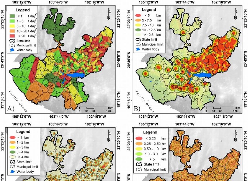
Sustainability 2020, 12, 3527                                                                                     3 of 32

compared to raw manure, and can be effectively used by crops [30–32]. Ammonium nitrogen also
shows a strong sorption capacity as it binds to soil sorption complexes, making it less prone to leaching
but still available for plant absorption [33,34].

1.2. Livestock Waste Importance and Pollution in Jalisco, Mexico
      Livestock waste can become valuable when it is managed correctly, but in Mexico manure is
currently one of the main sources of air, soil, and water pollution [35–37]. Mexico is the main emitter of
greenhouse gases in Latin America and the only one that is among the 15 highest pollutant-generating
nations [38]. Of Mexico’s total GHG emissions in 2015, 10% originated from livestock production
systems [39] Furthermore, poor agricultural practices promote runoff that contaminates surface and
groundwater, which is coupled with the fact that the Mexican territory has slopes that make it
susceptible to hydric erosion [40].
      Jalisco is one of 32 states in Mexico. It is in the center-west region of the country and has an
area of 78,588 km2 [41]. In 2018 Jalisco had a reported population of more than 8.1 million people
distributed among urban (87.9%) and rural (12.1%) areas [42]. Jalisco is the state that produces the
most food at a national level, and is the number one producer of certain goods, such as swine, eggs,
and milk [43]. INEGI (The National Institute of Statistics and Geography) reported 3,348,965 head of
beef, 2,766,180 head of swine, and 78,521,604 head of poultry for the state of Jalisco in 2017. These high
food production rates also make Jalisco the main generator of agricultural waste, which translates into
a serious environmental problem if not managed properly. On the other hand, with the right treatment
waste could become an economic advantage because of the fertilizer it could produce, and the thermal
and electrical energy potential it offers. According to the Law of Integral Management of Waste in
Jalisco (2007), every agricultural company must integrate biodegradable waste into their productive
processes, using it as an energy source or compost so it does not damage the environment [44].
      Jalisco’s hydrological system (Figure 1) has undergone a process of eutrophication, particularly
throughout the Lerma-Santiago basin [45,46]. Several researchers agree that more than 80% of the water
bodies in Jalisco are severely polluted, although none to the same degree as the Santiago River, which
frequently presents anoxic conditions [45,47,48]. Anoxic conditions develop when the consumption
of oxygen by biological or chemical processes exceeds the rate of resupply by vertical mixing and
diffusion, and in many cases it is associated with the runoff of nitrates from fertilizers [49–51]. Lakes
such as Cajititlán, Zapotlán, and Chapala present a high degree of eutrophication as reported in several
studies [45,52–55].
       Sustainability 2017, 9, x FOR PEER REVIEW                                                            4 of 34

                        Figure 1. Hydrological regions of the state of Jalisco (within national context).
                    Figure 1. Hydrological regions of the state of Jalisco (within national context).

       1.3. Cluster Spatial Analysis for the Anaerobic Treatment of Livestock Waste
            In recent years, an increasing awareness that AD can help mitigate odor, assist in nutrient
       recovery, and offer economic benefits, has stimulated renewed interest in the technology [22,56,57].
       Animal waste has the potential to be valorized and because these resources tend to be highly site-
       specific, it is important to know their location as well as the quantity produced [21,22,58].
       Governments and industries around the world have done research into clustered energy schemes of
       AD [21,22]. Given that geographical data and spatial factors (biomass availability, transportation
       distances, urbanization of the area, road infrastructure, protected areas, and environmental features)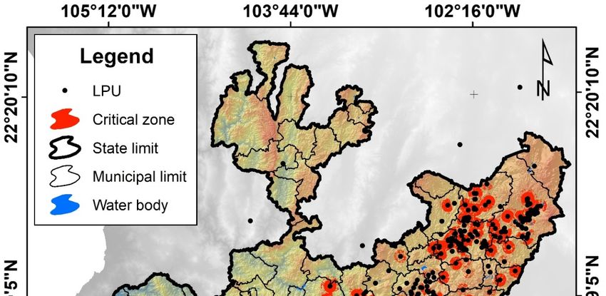
Sustainability 2020, 12, 3527                                                                       4 of 32

1.3. Cluster Spatial Analysis for the Anaerobic Treatment of Livestock Waste
     In recent years, an increasing awareness that AD can help mitigate odor, assist in nutrient recovery,
and offer economic benefits, has stimulated renewed interest in the technology [22,56,57]. Animal
waste has the potential to be valorized and because these resources tend to be highly site-specific, it
is important to know their location as well as the quantity produced [21,22,58]. Governments and
industries around the world have done research into clustered energy schemes of AD [21,22]. Given
that geographical data and spatial factors (biomass availability, transportation distances, urbanization
of the area, road infrastructure, protected areas, and environmental features) play a central role in
identifying optimal locations for siting biogas plants, geographic information systems (GIS) have
been used in previous studies [22,56–59]. Some studies have also analyzed the spatial distribution of
potential biomass feedstock in order to identify optimal locations for biogas plants [59–62].
     For these reasons, it is evident that agricultural waste, specifically animal manure, has greatly
contributed to water and air pollution in Jalisco. Nonetheless, improving manure management has
the potential to improve the economics of agriculture; this is dependent on spatial targeting of key
contributing areas [63,64]. Spatial analysis applied to manure management of farm clusters can
have positive impacts on economic and environmental factors, especially for small and medium
livestock production farms [65,66]. Cost-effective benefits are presented considering that the expenses
of implementation can become a major obstacle if the optimization analysis is not done correctly. On
the other hand, cluster management can offer more control over waste pollutants and increase the
valorization potential of manure. Framing manure management as a geographical and mathematical
optimization problem can help find an appropriate solution that assists in reducing operational costs
and maximizing environmental efficiency [65]. The aim of this study is to assess the energetic, nutrient,
and environmental potential of livestock waste in Jalisco, considering the implications for the state’s
hydrological systems. As a contribution to the literature, the methodology proposed here implements
a weighted overlay analysis with specific weighted categories that account for both viability factors
and environmental parameters, in order to identify viable places to install centralized AD units, as well
as the most critical regions for reducing the environmental impact of the Jalisco livestock industry. A
system such as the one proposed here could help the state of Jalisco move closer to meeting its energy
demands and would offer small and medium livestock producers cheaper and more efficient treatment
for their waste, while also greatly reducing greenhouse gas emissions and nutrient pollution of soils
and water bodies, which are issues of great importance for the state.
     The proposed centralized anaerobic digestion units (CADUs) offer multiple benefits compared to
individual farm-based AD units, such as requiring a lower energy consumption and lower individual
investment. However, transportation costs greatly influence the operation and viability of CADUs and
spatial parameters must be considered in order to reduce transportation costs between CADUs and the
substrate providers, and between CADUs and the final consumers of the digestate process [67]. In this
study, the distance between the potential sites for CADUs and the nearest LPUs was considered for the
weighted overlay analysis, however, further studies should estimate transportation costs considering
also the distribution of the digestate from the CADUs to the final consumers as part of the weighted
overlay analysis. Other spatial parameters that could help improve the accuracy of the model include
the distance to the road infrastructure and electric grid. Proximity to an existing road network and to
the existing electrical grid would be, of course, advantageous. A wider range of substrates, such as
crop waste, should also be considered (for co-digestion) in future studies.

2. Methods
      The complete methodological approach used in this study is summarized on Figure 2.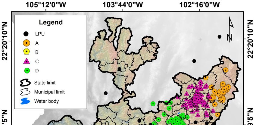
to an existing road network and to the existing electrical grid would be, of course, advantageous. A
       wider range of substrates, such as crop waste, should also be considered (for co-digestion) in future
       studies.

       2. Methods
Sustainability 2020, 12, 3527                                                                              5 of 32
       The complete methodological approach used in this study is summarized on Figure 2.

                                Figure 2. Graphical
                                   Figure 2. Graphicaldescription
                                                       description of the
                                                                      theproposed
                                                                          proposedmethodology.
                                                                                   methodology.

2.1. Data  Collection
      2.1. Data       andand
                Collection Processing
                              Processing

     Data related to the location and headcount of LPUs were obtained from historical records provided
by SEMADET (Environment and Land Development Agency) for registered livestock producers
updated to January 2019, in conjunction with records obtained from ANBIO (National Biomass Atlas).
All LPU locations and headcounts were verified to identify any errors in the dataset by calling the
registered numbers for the LPUs. Common errors found in the data were abnormal or incomplete
coordinates as well as incomplete or abnormal headcount data. These were all corroborated with
livestock producers and updated.
     Data used to determine the hydrographic structure of Jalisco, including both superficial water
bodies and surface runoffs, were obtained from INEGI and CEA (State Water Commission), available as
open access data. As for the data relating to the digital elevation model, location of urban communities,
municipal limits, and state limits, they were gathered from the official geographical data provided by
INEGI [68].
     A geographic information system was used to assess the location of the LPUs in Jalisco as well as
the hydrographic structure around them. A GIS is designed to spatially map resources and is valuable
for a wide range of public and private companies to plan strategies and manage infrastructure in a
region [69–71].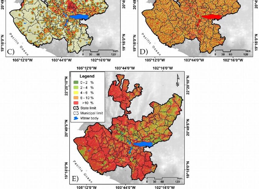
Sustainability 2020, 12, 3527                                                                       6 of 32

2.2. Identification of Critical Clusters
      Using the k-means clustering method in ArcGIS 10.5 software, ten initial clusters were defined in
order to group together the different LPUs scattered across the state. The k-means method allocates
each point to a specified number of clusters and attempts to minimize the global goodness-of-fit
measures by using a sum squared error (SSE). This measure is the distance from each point to the
centroid of the cluster [72]. Therefore, in the context of this study, clusters may be defined as spatial
groupings of LPUs that are close to each other.
      In order to identify the critical clusters and determine the locations for the CADUs we completed
a weighted overlay analysis. For this purpose, we generated a weighted index matrix to classify and
rank the rasters according to the specific parameters. Five parameters were evaluated in order to locate
priority zones for installing CADUs for farm clusters, taking into consideration total waste production
and environmental characteristics that favor pollutant transfer and superficial water pollution: (1) total
livestock waste produced by the LPU closest to the potential sites; (2) distance between the potential
sites and the nearest livestock production unit; (3) distance between the sites and the nearest urban
community; (4) distance between the sites and the nearest superficial water body; and (5) slope of the
sites. In this case, the parameters to assess the suitability of a given location for a CADU were selected
based on previous studies, as shown in Table 1. Several other spatial parameters have been included in
similar studies, such as distance to roads, to the electric grid, and to airports, and floodplains, among
others [21,22,56–59,73–76].

2.2.1. Total Livestock Waste Produced by the LPU Closest to the Potential Sites
     It is important to consider the size of the production unit located closest to the potential sites in
order to evaluate and categorize its impact on the surrounding areas, since higher amounts of waste
represent a higher risk of pollution. A small production unit, on the other hand, could lead to shortages
in the supply of the substrate for the CADU [77,78].
     To that end, total waste per species (Ti ) was calculated for each LPU according to Equation (1),
using total headcounts for each species in a specific LPU (Hi ) and the mean daily waste production
associated with poultry, cattle, and swine production (Ri ), which was estimated using reports from
multiple authors (presented in Table 2). The total daily waste production values corresponding to
poultry, cattle, and swine production were added to obtain the total daily waste production (Tw ) for
each LPU, as shown in Equation (2).
                                               Ti = Hi × Ri                                            (1)
                                                     X
                                                Tw =    Ti                                             (2)
Sustainability 2020, 12, 3527                                                                                                                                          7 of 32

      Table 1. Parameters used to assess the suitability of a given location for siting a centralized anaerobic digestion unit (CADU) reported in previous studies.
      LPU = livestock production unit.

                                              Total Livestock Waste   Distance between    Distance between the    Distance between the
                                                                                                                                          Slope of
                 Authors               Year   Production at Nearest    the Site and the   Site and the Nearest    Site and the Nearest                  Study Region
                                                                                                                                          the Site
                                                 LPU to the Site         Nearest LPU       Urban Community       Superficial Water Body
          Mukherjee et al. [73]        2015            X                     X                     X                       X                          Connecticut, USA
           Comber et al. [74]          2015            X                     X                                                                       East Midlands, UK
             Ma et al. [22]            2004            X                     X                     X                       X                 X         New York, USA
                                                                                                                                                        Buenos Aires,
         Venier and Yabar [56]         2017            X                     X                     X                       X
                                                                                                                                                         Argentina
               Zareei [75]             2018            X                     X                     X                       X                                Iran
     Dagnall, Hill, and Pegg [58]      2000            X                     X                     X                       X                                 UK
    Thompson, Wang, and Li [57]        2013            X                     X                     X                       X                 X         Vermont, USA
            Höhn et al. [59]           2014            X                     X                     X                                                  Southern Finland
   Batzias, Sidiras, and Spryou [21]   2005            X                     X                                                                             Greece
         Zubaryeva et al. [76]         2012            X                     X                     X                       X                 X       Apulia Region, Italy
Sustainability 2020, 12, 3527 8 of 32
Table 2. Waste production rates per species.
Waste Production Rates per Species (Ri )
Livestock kg head−1 day−1 kg head−1 month−1 kg head−1 year−1
Species
Value Average Range Value Average Range Value Average Range Source
31.6 960.96 11,534.00 [79]
36.98 1124.56 13,497.70 [80]
30.74 934.80 11,220.10 [81]
Cattle 35.37 30.74–47.70 1075.73 934.80–1450.55 12,911.26 11,220.10–17,410.5
32.50 988.33 11,862.50 [82]
47.70 1450.56 17,410.50 [83]
32.72 995.02 11,942.80 [84]
5.72 173.95 2087.80 [85]
11.47 348.80 4186.55 [79]
4.80 145.97 1752.00 [80]
Swine 8.03 4.80–15.15 244.39 145.96–460.71 2933.38 1752.00–5529.75
15.15 460.71 5529.75 [82]
6.03 183.37 2200.95 [84]
5.05 153.57 1843.25 [86]
0.35 10.64 127.75 [85]
0.10 3.04 36.50 [79]
0.25 7.60 91.25 [80]
Poultry 0.19 0.09–0.35 5.73 2.73–10.64 68.74 32.85–127.75
0.17 5.17 62.05 [82]
0.17 5.17 62.05 [84]
0.09 2.74 32.85 [86]Sustainability 2020, 12, 3527 9 of 32
2.2.2. Distance between the Potential Sites and the Nearest Livestock Production Unit
Just like the total waste produced, the distance between the site and the nearest LPU also affects
the feasibility of the project, given that long distances between the sites will translate into higher
transportation costs for collecting the substrates for the CADU. Additionally, locations closer to an
LPU suffer from higher levels of pollution since most producers dispose of their waste near the site
where it is generated [75,87].
2.2.3. Distance between the Potential Sites and the Nearest Urban Community
LPUs located in the vicinities of urban communities can affect their surroundings and therefore
have a negative effect on the communities within their range. CADUs operating correctly have a
lower impact on the surrounding communities compared to places with poor management practices,
therefore they can be located closer to populated areas without affecting their inhabitants [88,89].
2.2.4. Distance between the Potential Sites and the Nearest Superficial Water Body
Generally, LPUs treat and dispose of their waste mainly by field application [90,91] and, as
previously mentioned, this causes multiple environmental issues. It is important to focus on sites
closer to superficial water bodies as waste deposited closer to runoffs, rivers, or lakes has a more direct
impact on the water quality of the whole basin. CADUs should not have leaks or infiltration as this
would decrease the commercially valuable byproducts that can otherwise be obtained. Furthermore, it
would represent a risk of surface water contamination [92,93].
2.2.5. Slope of Potential Sites
Steeper terrains will have higher levels of runoff compared to flatter terrains, which make them
more prone to causing higher environmental impacts through leakage or infiltration, since they can
reach superficial water bodies more quickly [88,93].
For each parameter, a raster was obtained. A raster is defined as a densely packed array of pixels,
each with a specific value or intensity assigned to it [94]. Thiessen polygons were generated based
on the total waste production calculated for the corresponding farms. These polygons were later
transformed into raster format. The distances between the potential sites and the nearest livestock
production unit, the potential sites and the nearest urban community, and the potential sites and
the nearest superficial water body were all transformed into raster format images by calculating the
Euclidean distance for each variable. The slope of the potential sites was calculated based on the digital
elevation model of the area and then converted into a raster format [95].
For the weighted index table (Table 3), each parameter was modeled and assigned suitability
values ranging from 1 to 5. The raster images were classified based on a 1–5 scale depending on how
these parameters increase the risk of pollution of the areas where they are located and the viability
of the implementation of CADUs; 1 represents the lowest risk and viability and 5, the highest. The
weight of each parameter was assigned based on reported studies [96–98] and experienced specialists
who were consulted for this particular exercise.
The weighted overlay analysis using the obtained raster images was done according to Equation (3),
where R is the resulting risk factor for each pixel in the resulting raster, Wi is the assigned weight for
each variable, and Vi is the value of the corresponding reclassified raster for each pixel.
X5
[(Wi∗Vi)] (3)
i=1Sustainability 2020, 12, 3527 10 of 32
As a result, a classification raster was obtained where each pixel is classified on a scale from 1 to 5
corresponding to the risk of environmental pollution resulting from management of livestock waste
and the viability of the implementation of CADUs based on the previously mentioned parameters.
The zones with scores of 5 were selected as critical zones, since they present the highest viability and
environmental risk factors.
Based on the weighted overlay analysis and the critical zones identified by it, the critical percentage
of each cluster was determined by calculating the percentage of LPU sites located in critical zones for
each of the previously proposed clusters. Clusters with 75% or more of their LPUs located in critical
zones were selected as critical clusters.
Table 3. Weighted index table.
Weight (%) Value
Parameter Unit
1 2 3 4 5
Total livestock waste
production at nearest Ton day−1 30 0–1 1–5 5–10 10–20 >20
LPU to the site
Distance between the
site and the nearest m 30 >2000 1500–2000 1000–1500 500–1000 0–500
LPU
Distance between the
site and the nearest m 10 >2000 1500–2000 1000–1500 500–1000 0–500
urban community
Distance between the
site and the nearest m 20 >500 300–500 100–300 50–100 0–50
superficial water body
Slope of the site % 10 0–2 2–4 4–6 8–10 >10
2.3. Critical Cluster Analysis
In order to evaluate the viability of implementing CADUs, the following parameters were selected:
total waste production; total nitrogen and phosphorus digestate recovery; methane production
potential; electric energy potential; and carbon dioxide equivalent (CO2 eq) reduction. These were all
calculated for the selected critical clusters and the municipalities that form them using bibliographical
considerations (Table 4). Calculations regarding waste generation per species, volatile solid fraction
in waste, and methane generation potential were done using the mean, minimum, and maximum
values reported in literature (Tables 2 and 4) in order to obtain the minimum, maximum, and average
estimates (Tables 6 and 7). The same values were calculated at a state level by adding together the
values found for all LPUs in the state inventory.Sustainability 2020, 12, 3527 11 of 32
Table 4. Volatile solid fraction and methane production rates per species.
Volatile Solid Fraction (Vs) (%) Methane Production (Mp) (Nm3 CH4 kg Volatile Solids−1 )
Livestock Species Value Average Range Source Value Average Range Source
10.79 16.80 [99]
0.24 0.19 [28]
16 [100]
28.8 [101]
Cattle 10.79–28.8 0.13 0.13–0.24 [28]
10.86 [84]
13.12 [102]
0.21 [103]
21.7 [104]
12.23 14.80 [99] 0.29
0.34 [28]
20 [100]
22 [101]
Swine 6.22–22 0.45 0.29–0.45 [28]
8.59 [84]
20.02 [102]
0.29 [103]
6.22 [28]
19.38 24.80 [99] 0.157
0.19 [28]
17 [100]
19.5 [101]
Poultry 17–37.21 0.023 0.02–0.39 [28]
19.11 [84]
37.21 [102]
0.39 [105]
36.7 [106]Sustainability 2020, 12, 3527 12 of 32
2.3.1. Nitrogen and Phosphorus Recovery
Using the waste production for each species for each individual LPU (which was previously
calculated), total nitrogen recovery per LPU (NT ) was found using Equation (4), where Nc represents
the nitrogen composition of each species’ waste and NT represents the total nitrogen recovery from an
individual LPU. For this study the Nc values used were 23.3, 30.8, and 51.0 g of nitrogen per kg of
waste for cattle, swine, and poultry respectively, as reported by Kirchmann and Witter [107].
X
NT = Nci × Ti (4)
Total phosphorus recovery per individual LPU (PT ) was calculated using Equation (5), where
PT represents the total phosphorus recovery per LPU and Pc indicates the weight fraction of the
phosphorus present in each species’ waste. For this study the Pc values used were 8.0, 29.1, and 21.1 g
of phosphorus per kg of waste for cattle, swine, and poultry respectively, as reported by Barnett [108].
X
PT = Pci × Ti (5)
Total nitrogen and total phosphorus recovery values for the selected critical clusters and their
corresponding municipalities were calculated by adding the total nitrogen and phosphorus recovery
values for each of the LPUs belonging to the cluster or municipality.
2.3.2. Energetic Potential Calculation
The percentage of volatile solids present in livestock waste (Vs) and the methane production from
volatile solids (Mp) were obtained (Table 4).
The total methane production (MT ) (reported in normal cubic meters, Nm3 ) for each LPU was
calculated based on the total volatile solid content in the waste produced by each species and the
methane production rates presented in Table 4, given that each species’ waste has a different composition
and therefore a different methane potential depending on the total volatile solids present in it. The
electrical energy potential for each LPU and for each CADU was calculated for two scenarios, as
presented in Table 5: (1) using its energetic potential and the most common conversion efficiency (ηA )
for small generators [109], where the total electrical potential is represented as EeA ; and (2) using its
energetic potential and the most common conversion efficiency (ηB ) for large generators [109], where
the total electrical potential is represented as EeB . For both scenarios, the total electrical potential was
calculated using the energetic capacity (Em ) of methane proposed by Cuellar [110].
X
MT = Vsi × Ti × Mpi (6)
EeA = ηA × MT × Em (7)
EeB = ηB × MT × Em (8)
The total methane potential and electric energy potential for the selected critical clusters and their
corresponding municipalities were determined under the two proposed scenarios by adding together
the values that were calculated for their corresponding LPUs.
2.3.3. Greenhouse Gas Emission Calculation and Potential Reduction
Greenhouse gas emissions for each individual LPU and CADU were calculated according to two
scenarios, as shown in Table 5:
(1) Calculating the amount of equivalent CO2 generated by the previously determined amount
of waste generated for each LPU if the waste is disposed of directly by field application—as this is
the most common practice in Jalisco [90,91]—represented as CA in Equation (9). NN2O represents
the fraction of the total nitrogen present in waste that is transformed into N2 O in field applicationSustainability 2020, 12, 3527 13 of 32
conditions. The CO2 equivalent conversion factors for methane and nitrous oxide used are the ones
proposed by the IPCC (Intergovernmental Panel on Climate Change) [111].
CA = (MT × 25 × 67) + (NT × NN2O × 298) (9)
(2) The second scenario was calculated for a situation in which the waste generated by each
specific LPU is treated by anaerobic digestion in a CADU and the biogas obtained through this process
is used for the production of electric energy. This is shown in Equation (10), where CB represents the
total equivalent CO2 for this scenario and Cm represents the equivalent CO2 emitted by the combustion
of methane during energy generation. Under anaerobic conditions, N2 O generation is substantially
reduced and can be considered negligible [112–114].
CB = MT × Cm (10)
Table 5. Proposed scenarios for greenhouse gas emission calculations.
Scenario Energetic Potential Calculation Greenhouse Gas Emission Calculation
Waste generated by the individual LPUs is
disposed of directly by field application, which is
The methane produced by the the most common practice in Jalisco. N2 O is
anaerobic digestion (AD) process is reportedly generated at a rate of 0.2 kg of N2 O
A transformed into electric energy by per kg of the nitrogen content of the waste. The
low efficiency small farm-scale CH4 generated by the uncontrolled degradation
generators (ηA = 25%) [109] of organic matter in soil is also considered. N2 O
and CH4 present values of 298 and 25 kg CO2eq
per kg, respectively [111,115].
Waste generated by each specific LPU is treated
by anaerobic digestion in a CADU and the biogas
obtained through this process is used for the
The methane produced by the AD production of electric energy. Since N2 O
process is transformed into electric generation can be negligible during controlled
B
energy by high efficiency centralized AD only CH4 generated during the AD process is
generators (ηB = 40%) [109]. taken into account. Additionally, as it is used for
energy generation, the CH4 is transformed into
CO2 by combustion at a rate of 2.75 kg of CO2 per
kg of CH4 [111,115].
The equivalent CO2 reduction (CR ) was estimated using Equation (11) to evaluate the difference
in the total CO2 equivalent generation between the two proposed scenarios.
CR = CA −CB (11)
Total CO2 equivalent generation for both scenarios and total CO2 reductions for the selected critical
clusters and their corresponding municipalities were determined by adding the values calculated for
the LPUs belonging to these clusters and municipalities.
The hypotheses explaining the differences between the A and B scenarios regarding electricity
potential and CO2 equivalent generation are summarized in Table 5.
3. Results
Five classificatory maps were created (Figure 3), one for each of the parameters evaluated with its
respective classificatory scale. As a result of the weighted overlay analysis, a general map (Figure 4)
was made, which indicates the critical zones within each of the initial clusters. These critical zones
were highlighted in red as they were assigned the highest possible grade based on the five parameters
that were evaluated, which consider environmental risks, CADU viability parameters, and the weightsSustainability 2020, 12, 3527 14 of 32
used (shown in Table 3). The total critical area (in red) determined was 5417.10 km2 , which amounts to
6.8% of the total territory of the state.
Sustainability 2017, 9, x FOR PEER REVIEW 17 of 34
Figure 3. Classification of raster images for: (A) Total livestock waste production from the LPU closest
Figure 3. Classification of raster images for: (A) Total livestock waste production from the LPU closest
to the potential sites. (B) Distance from the potential sites to the nearest livestock production unit. (C)
to the potential
Distancesites. (B)potential
from the Distance from
sites to thethe potential
nearest sites to the(D)
urban community. nearest
Distancelivestock production unit.
from the potential
(C) Distance
sitesfrom
to thethe potential
nearest sites
superficial to the
water nearest
body. (E) Site urban
slope. community. (D) Distance from the potential
sites to the nearest superficial water body. (E) Site slope.
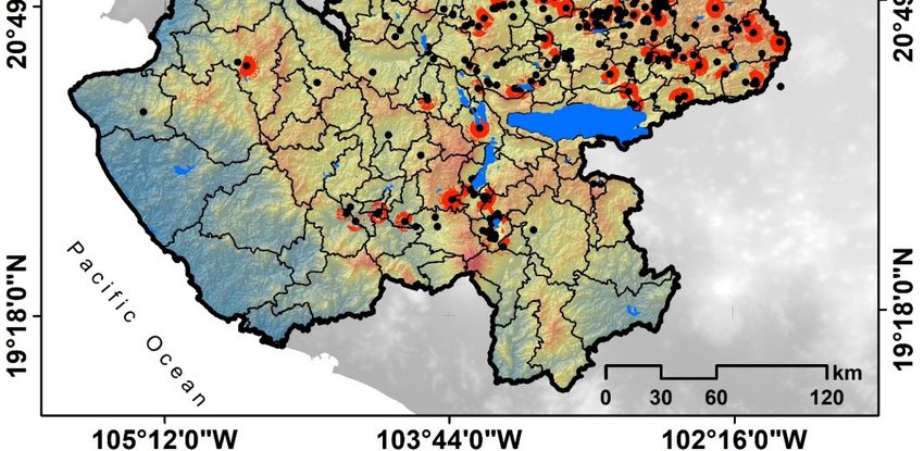
The percentage of LPUs located within the critical zone (or cluster) was determined for each
cluster. The clusters that were found to have 75% or more of their LPUs located within critical zones
were classified as critical clusters. Four clusters located in “Los Altos Norte” and “Los Altos Sur”
regions had 75% of their LPUs within critical zones. They were therefore identified as critical clusters,
and labeled A, B, C, and D as shown in Figure 5.
Tables 6–8 show total values for waste generation, nitrogen and phosphorus recovery, methane
production potential, electric energy potential under the two proposed scenarios, and equivalentSustainability 2020, 12, 3527 15 of 32
CO2 reduction for the selected critical clusters (where CADUs should be implemented) and the
municipalities that they make up (again, considering the two proposed scenarios). The table also
shows the total values at a state level. These values are not presented at the LPU level because the
focus of this work is on the viability of CADUs to collect wastes within the clusters.
Sustainability 2017, 9, x FOR PEER REVIEW 18 of 34
Figure 4. Critical zones identified in Jalisco as a result of the weighted overlay analysis.
4. Critical
Figure Sustainability zones identified in Jalisco as a result of the weighted overlay
2017, 9, x FOR PEER REVIEW
analysis.
19 of 34
The percentage of LPUs located within the critical zone (or cluster) was determined for each
cluster. The clusters that were found to have 75% or more of their LPUs located within critical zones
were classified as critical clusters. Four clusters located in “Los Altos Norte” and “Los Altos Sur”
regions had 75% of their LPUs within critical zones. They were therefore identified as critical clusters,
and labeled A, B, C, and D as shown in Figure 5.
Figure 5. Location of critical clusters within Jalisco.
Figure 5. Location of critical clusters within Jalisco.
Tables 6–8 show total values for waste generation, nitrogen and phosphorus recovery, methane
production potential, electric energy potential under the two proposed scenarios, and equivalent CO2
reduction for the selected critical clusters (where CADUs should be implemented) and the
municipalities that they make up (again, considering the two proposed scenarios). The table also
shows the total values at a state level. These values are not presented at the LPU level because the
focus of this work is on the viability of CADUs to collect wastes within the clusters.
With an estimated production of 4002.62 Gg per year, Jalisco is the largest producer of livestock
waste at a national level, compared to the waste production reported for the remaining 31 states [35].
From the estimated livestock waste total production, swine, poultry, and cattle production are
responsible for 61%, 28%, and 11% of waste generated, respectively.Sustainability 2020, 12, 3527 16 of 32
Table 6. Values calculated for critical clusters A and B.
Total Emission
Livestock Total Nitrogen Electricity Electricity
Phosphorus CH4 CO2 eq A CO2 eq B Reduction
Cluster Municipality Waste Recovery Potential Potential B
Recovery (Mg year−1 ) (Gg year−1 ) (Gg year−1 ) CO2 eq
(Gg year−1 ) (Mg year−1 ) A (MW) (MW)
(Mg year−1 ) (Gg year−1 )
Min 343.08 3930.44 2722.87 3398.79 0.97 1.55 108.39 9.35 99.05
Lagos de
Mean 594.53 7314.80 4865.64 19,266.00 8.21 13.13 512.29 52.98 459.31
Moreno
Max 1099.95 13,571.19 9085.67 76,328.91 21.78 34.85 1989.11 209.91 1779.20
Unión de Min 22.36 152.06 127.21 250.62 0.07 0.11 7.17 0.69 6.48
A San Mean 33.53 240.27 208.07 1039.09 0.44 0.71 26.73 2.86 23.88
Antonio Max 58.58 436.04 386.44 3373.17 0.96 1.54 86.93 9.28 77.65
Min 365.45 4082.50 2850.08 3649.41 1.04 1.67 115.57 10.04 105.53
Total A Mean 628.05 7555.07 5073.72 20,305.09 8.65 13.84 539.03 55.84 483.19
Max 1158.54 14,007.23 9472.11 79,702.08 22.75 36.39 2076.04 219.18 1856.85
Min 29.83 226.62 203.23 347.59 0.10 0.16 10.04 0.96 9.08
Atotonilco
Mean 47.36 369.96 337.03 1547.4 0.66 1.05 39.88 4.26 35.63
el Alto
Max 86.23 686.25 631.50 5097.45 1.45 2.33 131.53 14.02 122.44
Min 32.36 271.18 256.20 391.20 0.11 0.18 11.40 1.08 10.32
La Barca Mean 54.2 454.03 428.97 1850.5 0.79 1.26 47.76 5.09 42.67
Max 102.16 855.90 808.66 6166.73 1.76 2.82 159.27 16.96 148.95
Min 57.86 344.46 260.06 621.18 0.18 0.28 17.58 1.70 15.87
Ocotlán Mean 81.31 519.81 415.88 2356.38 1 1.61 60.48 6.48 54
Max 134.93 912.77 760.93 7496.59 2.14 3.42 192.85 20.62 176.98
B
Min 184.96 721.85 296.16 1774.70 0.50 0.81 48.67 4.88 43.79
Tototlán Mean 218.18 872.71 380.54 4960.16 2.11 3.38 126.02 13.64 112.38
Max 302.39 1249.00 581.33 14,428.91 4.12 6.59 368.17 39.68 324.38
Min 11.37 95.23 89.97 137.37 0.04 0.06–0.99 4.00–55.93 0.38–5.96 3.62–52.30
Zapotlán
Mean 19.03 159.44 150.64 649.81 0.28 0.44 16.77 1.79 14.98
del Rey
Max 35.88 300.55 283.97 2165.48 0.62 0.99 55.93 5.96 52.30
Min 316.39 1659.32 1105.63 3272.04 0.93 1.49 91.69 9.00 82.69
Total B Mean 420.08 2375.94 1713.05 11,364.25 4.84 7.75 290.91 31.25 259.66
Max 661.60 4004.47 3066.39 35,355.16 10.09 16.14 907.75 97.23 825.05
Values presented in bold represent the sum of the values reported for each individual municipality in the corresponding cluster.Sustainability 2020, 12, 3527 17 of 32
Table 7. Values calculated for critical clusters C and D.
Total Emission
Livestock Total Nitrogen Electricity Electricity
Phosphorus CH4 CO2 eq A CO2 eq B Reduction
Cluster Municipality Waste Recovery Potential Potential B
Recovery (Mg year−1 ) (Gg year−1 ) (Gg year−1 ) CO2 eq
(Gg year−1 ) (Mg year−1 ) A (MW) (MW)
(Mg year−1 ) (Gg year−1 )
Min 206.60 2435.94 1538.43 1906.13 0.54 0.87 62.17 5.24 56.93
Encarnación
Mean 352.66 4589.53 2791.53 11,063.63 4.71 7.54 296.45 30.42 266.02
de Díaz
Max 640.03 8456.62 5186.68 45,612.32 13.02 20.83 1190.71 125.43 1133.78
Min 580.95 7964.80 4898.05 5078.97 1.45 2.32 174.44 13.97 160.48
San Juan de
Mean 1049.83 15,431.17 9070.54 33,601.92 14.31 22.9 909.04 92.41 816.63
Los Lagos
Max 1947.94 28,585.88 16,893.80 145,769.25 41.60 66.56 3814.60 400.87 3654.13
Min 7.10 138.41 66.87 39.02 0.01 0.02 1.80 0.10 1.70
C
Teocaltiche Mean 14.05 284.53 133.79 431.13 0.18 0.29 12.17 1.19 10.98
Max 26.02 525.02 247.52 2278.55 0.65 1.04 60.09 6.27 58.40
Min 149.33 2515.21 1353.20 1056.25 0.30 0.48 41.40 2.90 38.49
Jalostotitlán Mean 284.71 5056.35 2615.32 8943.86 3.81 6.1 247.48 24.6 222.88
Max 529.26 9350.14 4855.01 43,283.50 12.35 19.76 1137.81 119.03 1099.32
Min 943.97 13,054.37 7856.55 8080.37 2.30 3.69 279.81 22.22 257.59
Total C Mean 1701.26 25,361.58 14,611.18 54,040.53 23.02 36.83 1465.13 148.61 1316.52
Max 3143.25 46,917.67 27,183.01 236,943.62 67.62 108.19 6203.22 651.59 5945.63
Min 54.51 492.62 436.33 637.50 0.18 0.29 18.87 1.75 17.12
Acatic Mean 92.25 848.83 740.5 3127.88 1.33 2.13 81.2 8.6 72.6
Max 173.70 1594.98 1393.79 10,806.85 3.08 4.93 279.68 29.72 262.56
Min 201.33 9024.47 1686.64 1872.81 0.53 0.86 62.25 5.15 57.10
Tepatitlán
Mean 359.93 4943.44 3076.59 11,652.53 4.96 7.94 312.87 32.04 280.82
de Morelos
Max 670.07 9175.12 5740.97 48,635.18 13.88 22.21 1270.56 133.75 1213.46
D
Min 32.78 306.42 167.07 290.22 0.08 0.13 9.08 0.80 8.28
Zapotlanejo Mean 49.66 554.22 298.94 1394.39 0.59 0.95 37.22 3.83 33.39
Max 82.61 993.04 544.69 5601.77 1.60 2.56 145.96 15.40 137.68
Min 288.61 3387.79 2290.05 2800.53 0.80 1.29 90.20 7.70 82.50
Total D Mean 501.85 6346.49 4116.03 16,174.8 6.89 11.02 431.29 44.48 386.81
Max 926.38 11,763.14 7679.45 65,043.82 18.56 29.70 1696.20 178.87 16,13.70
Values presented in bold represent the sum of the values reported for each individual municipality in the corresponding cluste.Sustainability 2020, 12, 3527 18 of 32
Table 8. Values calculated for critical clusters (total).
Total Total Emission
Livestock Electricity Electricity
Nitrogen Phosphorus CH4 CO2 eq A CO2 eq B Reduction
Waste Potential A Potential B
Recovery Recovery (Mg year−1 ) (Gg year−1 ) (Gg year−1 ) CO2 eq
(Gg year−1 ) (MW) (MW)
(Mg year−1 ) (Mg year−1 ) (Gg year−1 )
Sum Min 1914.42 22,183.98 14,102.31 17,802.36 5.08 8.13 577.28 48.96 528.32
Critical Mean 3251.23 41,639.08 25,513.98 101,884.68 43.4 69.44 2726.36 280.18 2446.18
Clusters Max 5889.77 76,692.50 47,400.96 417,044.68 119.02 190.43 10,883.20 1146.87 10,354.89
Min 2370.47 26,482.52 17,365.25 22,660.38 6.47 10.35 724.34 62.32.33 662.03
Jalisco Mean 4002.62 49,240.41 31,153.68 126,025.78 53.63 85.88 3354.19 346.57 3012.62
Max 7256.18 90,752.42 57,931.67 505,210.76 144.18 230.69 13,171.15 1389.33 12,509.12
Nc values used were 23.3, 30.8, and 51.0 g of nitrogen per kg of waste for cattle, swine, and poultry respectively, as reported by Kirchmann and Witter [107]. Pc values used were 8.0, 29.1,
and 21.1 g of phosphorus per kg of waste for cattle, swine, and poultry respectively, as reported by Barnett [108]. CO2 eq = carbon dioxide equivalent.Sustainability 2020, 12, 3527 19 of 32
With an estimated production of 4002.62 Gg per year, Jalisco is the largest producer of livestock
waste at a national level, compared to the waste production reported for the remaining 31 states [35].
From the estimated livestock waste total production, swine, poultry, and cattle production are
responsible for 61%, 28%, and 11% of waste generated, respectively.
4. Discussion
The multi-criteria GIS methodology suggests that CADUs should be located in four clusters
selected based on waste production and environmental features that favor pollutant distribution,
which led to an evident conglomeration of LPUs in Jalisco’s northeast region. This geographical area is
located in the hydrological region of the Lerma-Santiago-Chapala basin. As previously discussed, the
basin is undergoing eutrophication, which has been shown to be related to livestock production and
agricultural practices [45,48]. The degree of eutrophication of water bodies was not a parameter for the
selection of the clusters; however, the cluster analysis shows that the critical zones that were selected
are also the ones with the highest levels of water pollution [47]. Although there are several other
factors to consider, this can be strong evidence of the environmental damage that can be caused by poor
livestock and agricultural management practices, since inadequate management is known to produce
large quantities of nitrogen, phosphorus, and other nutrients that are key to eutrophication processes
in water bodies [116]. The methodology presented in this study could be improved by including
additional environmental, economic, and social parameters, as well as an economic optimization
framework. A SWOT (strengths, weaknesses, opportunities and threats) analysis is presented for the
methodology used in this study (Table 9).Sustainability 2020, 12, 3527 20 of 32
Table 9. SWOT (strengths, weaknesses, opportunities and threats) analysis table.
Favorable Unfavorable
Strengths Weaknesses
It is a quantitative methodology that makes it possible to identify and classify
LPU clusters in a given region in areas of high environmental risk and with The application of the methodology may be subjective (i.e., it requires the
the most viability for CADU implementation as a result of the weighted judgment of experts to select the parameters and to determine their weights).
overlay analysis. The results not only indicate where resources are available The analytic hierarchy process (AHP) may be used for selecting and weighting
based on spatial distribution, but also show where the best potential and the parameters, thus reducing bias in decision-making.
priority locations should be located in the future.
Other parameters may be considered for the analysis such as the proximity to
It is a flexible methodology that allows for the integration of a wide variety of the electric grid or to the road network, the preparedness of farmers to
environmental, economic, and social parameters to the spatial model to help participate, spatial water pollution levels, and a number of local factors not
determine the optimal sites for installing CADUs from a holistic perspective. included in this study. Additionally, the financial viability could be assessed
with the use of an economic optimization framework.
The mathematical models rely on actual farm data of location and headcount
Euclidean distance between the potential sites and the LPUs was used rather
of LPUs as well as actual data of the hydrographic structure of Jalisco, the
than the road network distance.
digital elevation model, and the location of urban communities.
Only livestock manure was used for the calculation of the biogas potential.
This methodology is rooted in multicriteria evaluation integrated with a
Information regarding the spatial distribution of a wider range of substrates
Internal geographical information system (GIS). The methodology can be easily
available in Jalisco for co-digestion could improve the estimation of the state’s
implemented with a medium level of GIS understanding.
potential for biogas production.
In this study only bibliographical considerations were used to determine the
precise methanogenic potential and nitrogen and phosphorus digestate
The application of this methodology has favorable repercussions in
composition. Experimental studies using biodigesters at the laboratory and
decision-making on environmental, social, health, and economic issues.
pilot levels must be carried out because substrates tend to be highly
site-specific.
The amount of energy produced by the CADUs represents only 3.4–5.5% of
the state’s energy consumption, so its scope will probably only satisfy local
The resulting graphical display is easily understandable for state/local energy demands. The results of this current study may be underestimated,
governments and other parties interested in biogas energy potential, and it being that the total headcount according to SADER (Agriculture and Rural
serves as guide for planning investment in any local region. Development Agency) is 3.22, 89.10, and 7.47 times higher for swine, cattle,
and poultry, respectively. However, the data estimated by SADER lacks the
LPU location information necessary for the spatial analysis.
Potential stakeholders interested in the implementation will need the CADUs
With the implementation of CADUs, more farms can use a large facility and
to be connected to the grid. Such a connection can be costly if locations are not
economies of scale can be achieved. Farmers need new ways to comply with
close enough to the existing electrical grid. This parameter should be included
increasing federal and state regulation of animal wastes.
for the weighted overlay analysis in future studies.Sustainability 2020, 12, 3527 21 of 32
Table 9. Cont.
Favorable Unfavorable
Opportunities Threats
This methodology allows for a first approach to a future implementation. A poor selection of the panel of experts defining and weighing the parameters
However, the participation of different stakeholders would be necessary for a can translate into misleading results with economic, social, and environmental
refining phase. consequences.
A wider range of substrates could be included in the analysis, although a
comprehensive assessment is required to understand how a wider range of If the information collected in the databases is not reliable, the level of
local substrates and substrate mixtures would affect the overall biodigester uncertainty in the results increases markedly.
operation.
The methodology can be easily adapted to other fields of application such as Transporting manure poses certain risks to the environment and public health
identifying sites for managing urban solid waste, siting collection centers and such as spillage of liquid or solid manure due to filtering, overloading,
processing food surpluses, and locating sites for managing waste from the blowing winds, or equipment breaking. Appropriate transportation
External tequila industry, among others. techniques should be applied.
The best practices for waste management should be encouraged at the It is important to visualize possible changes in energy policy at the federal
municipal and intermunicipal level for recycling and energy recovery, to level before deriving policy recommendations. Unfavorable electricity sale
promote farmers to become more interested in its implementation. tariffs may become a disincentive for future development of CADUs.
A broader benefit–cost analysis to determine the optimal locations based on
the capacity of the CADUs should involve the comparison of benefits and Biogas production requires facilities with personnel with medium to high
costs associated with pollution, to compare the economic costs of levels of technological skills. A lack of trained personnel could be a problem
implementing CADUs against the environment, and the health costs of not for further project implementation.
implementing them.
The state of Jalisco is the third largest consumer of electrical energy in Mexico
with 13,476.20 GW/h and it generates only 12% of that amount. The
production of energy through CADUs contributes to improving the energy
sufficiency of the state [117].Sustainability 2020, 12, 3527 22 of 32
Jalisco produces only 12% of the energy the state requires, which means it is compelled to import
88% of its energy from neighboring states, like Nayarit [118]. The total energetic potential of Jalisco’s
livestock waste represents 3.4% or 5.5% of the total energetic consumption reported for Jalisco in
2016 [119], with 53.68 MW and 85.68 MW for the two scenarios presented, with 25% and 40% efficiency
generation, respectively. By generating electric energy from livestock waste Jalisco can increase its
energy production by 28.7% or 45.8% for these scenarios, respectively. This could add up to Jalisco
producing a total of 15.45% or 17.5% of the energy it requires. The state has set the goal of producing
80% of its electrical energy demand by 2024 [119] and utilizing livestock waste as an energy source can
help the state move closer to meeting this goal. Cluster C, which among the four identified clusters
showed the highest energetic potential, has a total energetic potential calculated to be between 23 and
36.8 MW; that is, almost enough to cover 1.5% or 2.4% of Jalisco’s energy demand. Comparing the
results for the proposed A and B scenarios for energy generation calculations makes it clear that an
estimated 62% increase in the overall energy generated can be achieved by increasing the conversion
efficiency by using larger centralized generators rather than small-scale farm generators.
In addition to methane production and electricity generation, anaerobic digestion generates
valuable digestate. Compared to crude untreated manure, this digestate contains different nitrogen
and phosphorus compositions with higher availability for crops and presents higher sorption rates,
mainly due to the fact that the forms and proportions in which they are present change during the AD
process [33,34,120]. Moreover, since it is generated as a liquid sludge, it makes it possible to concentrate
the nutrient load by humidity reduction and simplifies transportation and field application [121].
This liquid fertilizer offers better infiltration rates compared to compost and inorganic fertilizers by
reducing nitrogen volatilization and improving crop nutrient absorption [122]. The total amount
of nitrogen produced by the livestock industry of Jalisco is comparable to the estimated nitrogen
required to fertilize Jalisco’s cultivated land. The total nitrogen produced per year could be utilized to
fertilize approximately 259,160 ha of maize fields [123]. While this might be promising, taking into
consideration that the approximate area dedicated to maize cultivation alone is 7,441,000 ha [124] and
almost 84% of the fertilizers needed at a national level must be imported [125], the field application
of untreated livestock waste loses its economic advantage compared to inorganic fertilizers due to
increasing transportation costs. Furthermore, it leads to the accumulation of waste in the fields
surrounding LPUs [126]. Digestate produced by CADUs, on the other hand, makes it possible to reduce
transportation and application costs compared to untreated livestock waste, while keeping production
costs lower than those of inorganic fertilizers. The volume and mass reduction of digestate is key
to making it easily transportable by reducing its bulk water content and concentrating its nutrients.
Simple solid–liquid separation methods like screen separators offer low separation rates at low costs,
whereas more advanced methods like screw pressing and decanter centrifugation offer better separation
rates at higher costs. These separation methods might be favorable in the case of CADUs given that
higher volumes of waste often reduce overall separation costs while maintaining separation rates [121].
Further humidity reduction can be achieved by a sequential drying process using waste-heat generated
from the conversion of the chemical energy of biogas into electrical and mechanical energy. This would
reduce transportation costs without greatly increasing treatment costs [121]. Multiple drying options
have been developed to reduce the water content of the generated digestate in order to concentrate its
nutrients and reduce transportation costs; belt drying, drum drying, and solar drying are some of the
most commonly used methods, followed by thermal vaporization [127].
Multiple models for determining the viability of manure application as a substitute for inorganic
fertilizer have been designed for high livestock waste-producing regions in order to prevent nutrient
accumulation in nearby fields. The increase in transportation costs has been linked to the high
volume of waste required to match the nutrient content of traditional inorganic fertilizers (since
waste has a high humidity content), and even though manure is generally cheaper than inorganic
fertilizers, transportation and application costs increase its total cost [128,129]. Jalisco’s total phosphorus
production has the potential to fertilize 519,228 ha of maize crop fields [130], but the same situationYou can also read