Evaluation of Multi-Stream Fusion for Multi-View Image Set Comparison - MDPI
←
→
Page content transcription
If your browser does not render page correctly, please read the page content below
applied
              sciences
Article
Evaluation of Multi-Stream Fusion for Multi-View Image
Set Comparison
Paweł Piwowarski                and Włodzimierz Kasprzak *

                                          Institute of Control and Computation Engineering, Warsaw University of Technology, 00-665 Warsaw, Poland;
                                          pawel@piwowarski.com.pl
                                          * Correspondence: w.kasprzak@elka.pw.edu.pl

                                          Abstract: We consider the problem of image set comparison, i.e., to determine whether two image sets
                                          show the same unique object (approximately) from the same viewpoints. Our proposition is to solve
                                          it by a multi-stream fusion of several image recognition paths. Immediate applications of this method
                                          can be found in fraud detection, deduplication procedure, or visual searching. The contribution of
                                          this paper is a novel distance measure for similarity of image sets and the experimental evaluation
                                          of several streams for the considered problem of same-car image set recognition. To determine a
                                          similarity score of image sets (this score expresses the certainty level that both sets represent the same
                                          object visible from the same set of views), we adapted a measure commonly applied in blind signal
                                          separation (BSS) evaluation. This measure is independent of the number of images in a set and the
                                          order of views in it. Separate streams for object classification (where a class represents either a car
                                          type or a car model-and-view) and object-to-object similarity evaluation (based on object features
                                          obtained alternatively by the convolutional neural network (CNN) or image keypoint descriptors)
                                          were designed. A late fusion by a fully-connected neural network (NN) completes the solution. The
                                          implementation is of modular structure—for semantic segmentation we use a Mask-RCNN (Mask

                                   regions with CNN features) with ResNet 101 as a backbone network; image feature extraction is
                                          either based on the DeepRanking neural network or classic keypoint descriptors (e.g., scale-invariant
Citation: Piwowarski, P.; Kasprzak,
                                          feature transform (SIFT)) and object classification is performed by two Inception V3 deep networks
W. Evaluation of Multi-Stream Fusion
                                          trained for car type-and-view and car model-and-view classification (4 views, 9 car types, and 197 car
for Multi-View Image Set
Comparison. Appl. Sci. 2021, 11, 5863.
                                          models are considered). Experiments conducted on the Stanford Cars dataset led to selection of the
https://doi.org/10.3390/app11135863       best system configuration that overperforms a base approach, allowing for a 67.7% GAR (genuine
                                          acceptance rate) at 3% FAR (false acceptance rate).
Academic Editor: Santiago Royo
                                          Keywords: image sets; set similarity metric; same object verification; same view verification; Deep-
Received: 17 May 2021                     Ranking; BSS error index
Accepted: 22 June 2021
Published: 24 June 2021

Publisher’s Note: MDPI stays neutral      1. Introduction
with regard to jurisdictional claims in
                                               By “visual similarity”, we understand that the visual content of two images, i.e.,
published maps and institutional affil-
                                          pictured objects, is the same or somehow similar. This type of comparison is not highly
iations.
                                          challenging if photographs of the same object are taken from the same place, so that they
                                          differ by only a few details. A typical solution to such a task is to extract standard image
                                          features or descriptions (embedding vectors) generated by deep neural networks, and to
                                          classify them or to apply a hand-crafted decision by using vector–distance metrics (i.e.,
Copyright: © 2021 by the authors.
                                          the Euclidean distance in vector space) [1,2]. The same image similarity problem becomes
Licensee MDPI, Basel, Switzerland.
                                          more difficult if the image content is a 3D object and the compared images present it from
This article is an open access article
                                          different viewpoints (Figure 1).
distributed under the terms and
                                               Direct comparison or classification of entire images (i.e., a front-to-end approach)
conditions of the Creative Commons
                                          by deep neural networks is a recent approach to image analysis [3–6] that has produced
Attribution (CC BY) license (https://
                                          outstanding results. However, consider the problem of defining the “similarity” of two
creativecommons.org/licenses/by/
4.0/).
                                          image sets and combine it with the problem of identifying the same “semantic” content,

Appl. Sci. 2021, 11, 5863. https://doi.org/10.3390/app11135863                                              https://www.mdpi.com/journal/applsci
set comparison system can improve the quality and speed of the claim handling process.
The growing demand for visual similarity solutions is clear and comes from companies
which seek effective answers for the aforementioned business problems. In recent years,
some significant papers have been published about this topic. The first one mentioned
Appl. Sci. 2021, 11, 5863 here gives a review of a few methods developed for finding similar images in datasets 2 of[7].
14
Another important paper proposes a deep learning technique for the image similarity task
Appl. Sci. 2021, 11, x FOR PEER REVIEW 2 of 14
called “DeepRanking” [8].
same
i.e., In3D
the this
same paper,
object we propose
3Dvisible
object from different
visible a solution
from differentto the
viewpoints. imageThisset
viewpoints. comparison
complex
This problem
complex problem
appears
problem (Figure
in vari-
appears 2).
in
This
ous problem
real-world is analyzed
business in Section
scenarios, 2, while
i.e., the
fraud proposed
detection, solution
various real-world business scenarios, i.e., fraud detection, visual navigation, productvisual is described
navigation, orin Section
product
3. Our approach
search. uses both
useful
It is also useful in imagesearch
in visual
visual (moreor
search exactly:
or foregroundavoidance—for
data duplication
data duplication object) classification
avoidance—for example,
example, andin ob-
in aa
ject-pair similarity evaluation procedures, and places
insurance application process. A customer would have to take a set
car insurance them in a general-purpose
set of
of photos
photos of frame-
of the
the
work
car system
in order
order to tofor
forimage-set
for the
the insurance
insurance comparison.
policy
policy totoThe
start,solution
start, and
and after requires
after an not only
an insurance
insurance eventthehappens,
event use of some
happens, the
the
category-level
customer
customer would would similarity,
have but
havetototake also
takeanother an instance-to-instance
another setsetofof
photos
photos of of
thethe metric.
samesame car.Thus,
AnAn
car. theautomatic
similarity
automatic image score
imageset
combines
comparison
set comparison thesystem
evaluation
can can
system of the
improve visual
improve content
the quality
the of image
and
quality speed
and pairs
of the
speed with
of thethe
claim comparison
handling
claim handling of
process. image
The
process.
features
growing computed
demand forfrom
visual object ROIs
similarity (region
solutions ofisinterest;
clear and
The growing demand for visual similarity solutions is clear and comes from companiesthe regions
comes from in the image
companies which
which
provide
seek
which theeffective
effective
seek needed
answers information).
for the for
answers We expect business
aforementioned
the aforementioned that the proposed
problems.
business solution
In recent
problems. Inmight
years,be
recent somede-
years,
ployed
significant for papers
some significantcomparisons
have been
papers of
havesets of images
published
been showing
about
published this cars,
topic.
about cats,
The
this buildings,
first
topic. one etc.one
Thementioned
first Anmentioned
earlier
here de-
gives
aveloped
review
here gives base solution
ofaareview
few of atofew
methods the same problem
developed
methods is referred
for finding
developed similar
for toimages
finding insimilar
Section 4. Theinexperimental
in images
datasets [7]. Another
datasets [7].
important
verification paper
Another important of our proposes
approach a deep
paper proposes learning
is summarized technique
a deep learningin Section for5.the
technique Theimage thesimilarity
presentation
for of task called
limitations
image similarity task
“DeepRanking”
and
calledconclusions
“DeepRanking”[8].
as well[8].
as a final discussion complete this paper.
In this paper, we propose a solution to the image set comparison problem (Figure 2).
This problem is analyzed in Section 2, while the proposed solution is described in Section
3. Our approach uses both image (more exactly: foreground object) classification and ob-
ject-pair similarity evaluation procedures, and places them in a general-purpose frame-
work system for image-set comparison. The solution requires not only the use of some
category-level
Figure similarity, but(object-to-object)”
1. The “image-to-image also an instance-to-instance
comparison problem
comparison metric.in
problem Thus,
in the similarity score
images.
images.
combines the evaluation of the visual content of image pairs with the comparison of image
In this
features paper, we
computed propose
from objecta ROIs
solution to theofimage
(region set the
interest; comparison
regions in problem
the image (Figurewhich 2).
This problem
provide is analyzed
the needed in Section 2,
information). Wewhile the proposed
expect solution issolution
that the proposed described in Section
might be de- 3.
Our approach uses both image (more exactly: foreground object)
ployed for comparisons of sets of images showing cars, cats, buildings, etc. An earlier de- classification and object-
pair similarity
veloped evaluation
base solution to the procedures,
same problem and places them to
is referred in in
a general-purpose framework
Section 4. The experimental
system for image-set
verification comparison.
of our approach The solution
is summarized inrequires
Section not5. Theonlypresentation
the use of some category-
of limitations
level similarity, but
and conclusions as also
wellan as instance-to-instance
a final discussion complete metric. Thus, the similarity score combines
this paper.
the evaluation of the visual content of image pairs with the comparison of image features
computed from object ROIs (region of interest; the regions in the image which provide
the needed information). We expect that the proposed solution might be deployed for
comparisons of sets of images showing cars, cats, buildings, etc. An earlier developed base
solution to the same problem is referred to in Section 4. The experimental verification of
our approach is summarized in Section 5. The presentation of limitations and conclusions
Figure
as well1.asThe “image-to-image
a final (object-to-object)”
discussion complete this paper.comparison problem in images.
Figure 2. The “object set-to-object set” comparison problem.
The main objective is to provide answers to questions such as “is my set of images
presenting the same object from the same viewpoint as the other set of images”. The object
is application-dependent. The exact recognition of views and objects in particular images
is not the question—the ultimate challenge is how to define a similarity measure for sets
of object-centered images. During the search for a solution to this problem, we discovered
that this case is nearly identical to the evaluation of multi-channel blind signal separation
results [9], where the objective is to specify whether the set of M signals extracted from N
mixtures is properly representing a (potentially unknown) set of M source signals. Our
Figure 2. The
Figure 2. The “object
“object set-to-object
set-to-object set”
set” comparison
comparison problem.
problem.
The main objective is to provide answers to questions such as “is my set of images
The main objective is to provide answers to questions such as “is my set of images
presenting the same object from the same viewpoint as the other set of images”. The object
presenting the same object from the same viewpoint as the other set of images”. The object
is application-dependent. The exact recognition of views and objects in particular images
is not
is application-dependent. The exact
the question—the ultimate recognition
challenge is howoftoviews
defineand objects inmeasure
a similarity particular
for images
sets of
is not the question—the ultimate challenge is how to define a similarity measure
object-centered images. During the search for a solution to this problem, we discovered for sets
of object-centered
that images.
this case is nearly During
identical the evaluation
to the search for aofsolution to this problem,
multi-channel we discovered
blind signal separation
that this
results case
[9], is nearly
where identicalistotothe
the objective evaluation
specify whetherof multi-channel blind extracted
the set of M signals signal separation
from N
results [9], where the objective is to specify whether the set of M signals extracted from N
mixtures is properly representing a (potentially unknown) set of M source signals. Our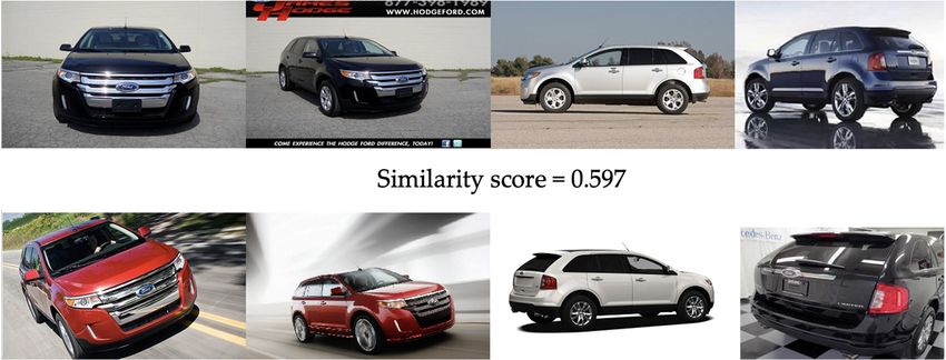
Appl. Sci. 2021, 11, 5863                                                                                            3 of 14

                            mixtures is properly representing a (potentially unknown) set of M source signals. Our
                            BSS-based similarity score takes into account object instances. We assume that other data
                            analysis streams can support this process by considering the consistency of object types
                            and views in both compared sets.
                                The contribution can be summarized as follows:
                            •    a fusion of several image processing and classification streams is proposed to solve
                                 the problem of set-to-set similarity evaluation;
                            •    a BSS error index [9]-based permutation-independent similarity score is proposed;
                            •    the advantage of using a DeepRanking network [8], with its triplet loss function for
                                 image feature extraction and image-pair similarity, is confirmed in comparison with
                                 classic SIFT features [10];
                            •    a quality improvement of a previous baseline approach is shown.

                            2. Problem and Related Work
                            2.1. Assumptions
                                  Let us make some assumptions to constrain the general problem of image set com-
                            parison. First, we constrain the kind of 3D objects we would like to identify and compare.
                            Here we shall distinguish the “image type” from “object type or category” and from the
                            “context”. The question, “are the images of the same type?”, asks whether the object views
                            are the same, i.e., a “front view” and a “side view” are examples of image types. The
                            question, “are the visual objects of the same type?”, is related to single foreground ob-
                            jects detected in the image and classified according to our “context” (application domain).
                            Object “categories” are generalizations of some types having the same basic properties.
                                  Examples of object types in the category of “cars” can be: “vans”, “sedans”, “trucks”,
                            and “lorries”. Examples of an application domain (context) are: cars for fraud detection
                            for insurance companies or buildings and other urban infrastructure for visual navigation.
                            The context can refer to single object categories (e.g., cars) or many object categories that
                            can appear in the same image (e.g., “a car next to the tree” or “a car on the bridge”). In this
                            work, we focus on the context of single cars present in an image.

                            2.2. Related Work
                                The primary problem of matching two image sets can be divided into subproblems
                            such as:
                            •    semantic segmentation (detection of the foreground object’s ROI),
                            •    feature extraction,
                            •    image-to-image similarity evaluation, and
                            •    image set-to-image set similarity evaluation.
                                  The literature doesn’t provide a complete solution to this problem, but we can find
                            several papers related to these subproblems. The “DeepRanking” approach [8] is a com-
                            prehensive solution based on deep learning (DL) technology that provides both feature
                            extraction and similarity evaluation of two images. We shall describe it in-detail in Section 4.
                            The alternatives for the DL-based features can be hand-crafted keypoint descriptors, such
                            as SIFT, speeded-up robust features (SURF), or “oriented features from accelerated segment
                            test (FAST) and rotated binary robust independent elementary features (BRIEF)” (ORB) [10].
                            Several methods of this kind are compared in [11], paying attention to their performance
                            for distorted images. Nowadays, computationally efficient binary keypoint descriptors
                            dominate in real-time image analysis applications [12].
                                  The next subproblem, how to measure a distance between images (or feature vectors),
                            can be solved by the use of obvious metrics such as Euclidean, Manhattan, or Cosine
                            distance or another, more specific one, such as the Hausdorff metric [1].
                                  The evaluation of two image sets reminded us of the evaluation of blind source
                            separation (BSS) algorithms as applied to the image sources [9]. There we faced a similar
                            problem—every estimated output must have been uniquely assigned to a single source and,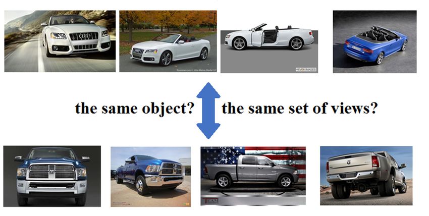
Appl. Sci. 2021, 11, 5863 4 of 14
in an ideal case, should not contain any cross-correlation with other sources. We proposed
an error index for both sets (separated outputs and reference sources) which handles the
possible differences in permutation (ordering of images in a set) and amplitude scales, and
is normalized by the number of set items.
Thus, our approach applies the DeepRanking-based DL stream of image pair compar-
ison, the SIFT descriptors as ROI features, and the Euclidean distance in a conventional
stream for image-to-image similarity evaluation. We also adapted the error index from BSS
research to estimate the image sets dissimilarity score.
The architecture of multi-stream fusion of data analysis streams that covers all of
the aforementioned subproblems into one final decision was chosen. The idea of such
architecture was previously proposed in [13]. Different works [14–16] deal with multi-view
image fusion to improve the results of single-view image analysis. The problems solved in
these papers are different from our problem, yet the idea of using different views to obtain
better results is close to our objective.
An overview of related papers, in accordance with a methodology to literature survey
and evaluation developed in [17–19], is shown in Table 1.
Table 1. An overview of related papers. X means “covered”. Citation count source is Google Scholar (last updated: 15 June
2021). Column explanation: I-2-I, set comparison based on comparison of image-to-image distance with Euclidean distance;
DR, DeepRanking as a feature extraction method; SIFT, SIFT as a feature extraction method; BSS, a blind signal separation
error index as a measure of the distance between two image sets; Car Model, a stream for car model classification.
Image Feature Multi Stream Analysis Image Set Comparison
Distance Measures
No of References
Reference No
Comparison
Segmentation
Classification
Citations
Car Model
Comparison
Extraction
Year
SIFT
I-2-I
BSS
DR
[1] 1999 167 23 X X X
[2] 2017 6 17 X
[3] 2013 1308 37 X
[4] 2013 38 23 X
[5] 2016 13861 23 X
[6] 2017 12098 35 X
[7] 2018 10 33 X X X
[8] 2014 1054 25 X X X X
[9] 1997 9 14 X X
[10] 2011 8238 30 X
[11] 2017 286 16 X X
[12] 2014 47 8 X
[13] 2018 27 40 X
[14] 2007 202 33 X
[15] 2020 6 34 X
[16] 2019 45 46 X
[20] 2014 16326 51 X X
[21] 2016 80936 49 X X
[22] 2015 7939 23 X X X
[23] 2007 49 39 X X
[24] 2021 - 11 X X X X X X X X X
Our 2021 - 25 X X X X X X X X X X X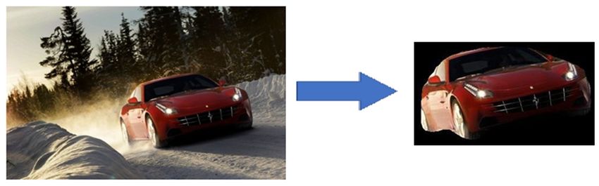
Our solution to image set similarity estimation is not limited by the number of im-
                            ages, and will be appropriate even for a single image pair. The core of this solution consists
                            of four image processing streams for image-pair comparison (Figure 3):

Appl. Sci. 2021, 11, 5863   1. the classification of the foreground object type,                                  5 of 14
                            2. the classification and the foreground object view,
                            3. image-pair similarity based on semantic image segmentation (the DL stream), and
                            4. feature-based image pair similarity (classic technique stream).
                            3. Solution
                                  After accumulating similarity scores obtained for all image-pairs from the two ana-
                            3.1.
                            lyzedStructure
                                    image sets, the individual results are fused and further classified to obtain a final
                                  Our solution
                             likelihood          to image
                                          as to whether    set sets
                                                         both  similarity
                                                                    containestimation
                                                                              the same is not limited
                                                                                        object.       by the number
                                                                                                The approach           of images,
                                                                                                                performs  a multi-
                            and  will  be  appropriate  even   for a  single image  pair. The   core of this solution consists
                             score “late fusion” (one possible approach to fuse multi-modal data, e.g., [14,15]), where        of
                            four  image   processing  streams
                             the following scores are fused:    for  image-pair   comparison    (Figure  3):
                            1.     the classification of the foreground object type,
                             1. The same-object (car)-type score (class likelihoods),
                            2.     the classification and the foreground object view,
                             2. The same-object (car)-model and -viewpoint score (class likelihoods),
                            3.     image-pair similarity based on semantic image segmentation (the DL stream), and
                             3. BSS error index (dissimilarity) based on all ROI image-to-image comparisons, and
                            4.     feature-based image pair similarity (classic technique stream).
                             4. BSS error index based on the ROI-features comparison for all image pairs.

                            Figure3.3.The
                            Figure    Thearchitecture
                                          architectureof
                                                       ofthe
                                                          theimage
                                                              imageset
                                                                    setcomparison
                                                                        comparisonapproach.
                                                                                   approach.

                             3.2. Image
                                  After Segmentation
                                          accumulating similarity scores obtained for all image-pairs from the two ana-
                            lyzedTheimage    sets,
                                         input      the individual
                                                image    sets alwaysresults   are fused
                                                                        have the         and further
                                                                                  same number         classified
                                                                                                  of images      to obtain
                                                                                                             (otherwise      a final
                                                                                                                           both  sets
                            likelihood     as to whether     both  sets  contain  the same   object.  The  approach
                             can immediately be declared as invalid). The Stanford Cars dataset [25] was used in ex-  performs     a
                            multi-score     “late  fusion”  (one  possible   approach   to fuse multi-modal    data, e.g.,
                             periments. It is a well-recognized car dataset providing model labels (annotation) and is     [14,15]),
                            where
                             cited inthe  following
                                       many           scores
                                               research       are fused:
                                                          papers.  It is freely available to the public and the attached annota-
                            1.tion reduces
                                   The same-object
                                           the effort(car)-type
                                                      needed for score (classdata
                                                                   training    likelihoods),
                                                                                   preparation. The order of the images is not
                            2.     The (the
                             relevant  same-object
                                            solution(car)-model    and -viewpoint
                                                      must be invariant               scoreto(class
                                                                           with respect        indexlikelihoods),
                                                                                                      permutation). We assume
                            3.     BSS error
                             that each       index
                                        set has     (dissimilarity)
                                                images               based
                                                         of four views:  theon   all ROI
                                                                              front,     image-to-image
                                                                                      side, front-side and comparisons,   and
                                                                                                            back-side view.  Alt-
                            4.
                             hough BSS
                                     inerror index
                                        general  ourbased   on the
                                                      approach   is ROI-features    comparisonuser
                                                                    view-independent—the          for all
                                                                                                       canimage pairs.
                                                                                                           decide to include any
                             other sets of views—in our opinion, and for the given dataset, these views are the best
                            3.2. Image Segmentation
                                  The input image sets always have the same number of images (otherwise both sets
                            can immediately be declared as invalid). The Stanford Cars dataset [25] was used in
                            experiments. It is a well-recognized car dataset providing model labels (annotation) and
                            is cited in many research papers. It is freely available to the public and the attached
                            annotation reduces the effort needed for training data preparation. The order of the images
                            is not relevant (the solution must be invariant with respect to index permutation). We
                            assume that each set has images of four views: the front, side, front-side and back-side view.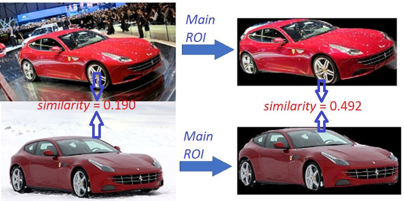
Appl. Sci. 2021, 11, 5863 6 of 14
Although
Appl. Sci. 2021, 11, x FOR PEER REVIEW in general our approach is view-independent—the user can decide to include 6 of 14
any other sets of views—in our opinion, and for the given dataset, these views are the best
selection. Our
selection. Our dataset
dataset does
does not
not have
have aa good
good representative
representative of of back
back view
view images—this
images—this is is
the reason why we do not consider such a view. Every image is labeled
the reason why we do not consider such a view. Every image is labeled by one of 4 views, by one of 4 views,
99 car
car types,
types, and
and 197
197 car
car models.
models. A A class
class label
label “other”
“other” isis also
also given
given toto images
images which
which dodo not
not
match any basic
match any basic class.class.
Image segmentation
Image segmentation follows
follows the
the semantic
semantic segmentation
segmentation approach
approach based
based on
on aa Mask-
Mask-
RCNN model [6]. To train the Mask-RCNN model, we used
RCNN model [6]. To train the Mask-RCNN model, we used the COCO dataset (2017 the COCO dataset (2017 ver-
sion) [20].
version) COCO
[20]. COCO contains
contains8181
categories
categoriesofofobjects
objectssufficient
sufficientforfor training
training and testing the
and testing the
entire model.
entire model.Semantic
Semanticsegmentation
segmentation removes
removes unnecessary
unnecessary partsparts of images
of images andkeeps
and only only
keeps
the thethat
parts partsare
that are consistent
consistent with
with the the created
created model model (application
(application context).
context). In partic-
In particular,
ular,
we we focus
focus on “Car”
on “Car” and and “Truck”
“Truck” categories
categories fromfrom
thethe
COCOCOCO dataset.The
dataset. TheMask-RCNN
Mask-RCNN
implementation uses
implementation uses aa ResNet
ResNet 101101 [21]
[21] neural
neural network
network architecture
architectureas asthe
thebackbone.
backbone.
In Figure
In Figure 4,
4, an
an example
example of of car
car mask
mask detection
detection results
resultsfrom
fromtwotwosteps:
steps:
1.
1. the rectangular
the rectangular boundary
boundary box
box for
for car
car region
region extraction
extraction comes
comes from
from the
the annotations
annotations
given in
given in the
the Stanford
Stanford Car
Car dataset,
dataset, and
and
2.
2. the Mask
the Mask RCNN
RCNN generates the proper
generates the proper envelope
envelope of
of the
the car
car image
image region
region within
within the
the
boundary box (from previous point).
boundary box (from previous point).
Figure 4.
Figure 4. Illustration
Illustration of
of car
car mask
mask extraction
extraction for
for car
car images
images from
from the
the COCO
COCOdatabase.
database.
3.3.
3.3. Detection
Detection of
of ROIs
ROIs
The
The ROIs detection step
ROIs detection step is
is the
the initial
initial step
step of
of two
two alternative
alternative streams
streams for
for set
set similarity
similarity
scoring,
scoring, based on deep neural networks or on classic key-point descriptors. WeWe
based on deep neural networks or on classic key-point descriptors. useuse
the
the Selective Search [4] algorithm to find ROIs in images. Selective Search uses
Selective Search [4] algorithm to find ROIs in images. Selective Search uses color, texture, color,
texture,
size, andsize, andmeasures
shape shape measures to characterize
to characterize image regions
image regions and iteratively
and iteratively to perform
to perform hierar-
hierarchical region grouping into ROIs. The list of obtained ROIs is ordered by area. We
chical region grouping into ROIs. The list of obtained ROIs is ordered by area. We prefer
prefer to skip the one with the biggest size and to select the next five (2nd–6th) for further
to skip the one with the biggest size and to select the next five (2nd–6th) for further anal-
analysis. We chose this selection to avoid the whole car ROI and to concentrate on a fixed
ysis. We chose this selection to avoid the whole car ROI and to concentrate on a fixed
number of meaningful ROIs. To obtain ROI similarity scores, their feature vectors are
number of meaningful ROIs. To obtain ROI similarity scores, their feature vectors are ob-
obtained by two alternative methods: DeepRanking and the SIFT-descriptor.
tained by two alternative methods: DeepRanking and the SIFT-descriptor.
3.4. DeepRanking Neural Network
3.4. DeepRanking Neural Network
Image-to-image comparison is a DL solution applied to foreground object ROIs de-
tectedImage-to-image comparison
in images. We measure is a DL solution
the Euclidean distance applied
betweento foreground
two embeddings objectproduced
ROIs de-
tected in images. We measure the Euclidean distance between two
by the CNN from the DeepRanking [8] approach. “FaceNet” was introduced in [22] and embeddings produced
by the CNN
proposed thefrom theloss
triplet DeepRanking
function as [8] approach.
a learning “FaceNet”
criterion. Thewas introduced
triplet in [22] and
loss minimizes the
proposedbetween
distance the triplet
theloss function
anchor (query as image)
a learning
andcriterion. Theexample
the positive triplet loss minimizes
image and maxi-the
distance
mizes thebetween
distancethe anchorthe
between (query
anchor image)and and the positive
the negative example
example image
image. and maxim-
DeepRanking
izes thethis
applies distance
tripletbetween
loss ideathe
to anchor
learn anand the negative example
image-to-image similarity image.
model. DeepRanking ap-
The triplet loss
plies this triplet loss idea to learn an
implementation in DeepRanking is as follows [8]: image-to-image similarity model. The triplet loss
implementation in DeepRanking is as follows [8]:
min ∑ ε i + λkWk22 s.t. : max 0, g + D f ( pi ), f pi+ − D f ( pi ), f pi−
min
i ‖ ‖ . . ∶ max 0, ( , ( − ( , ( (1)
< ε i ∀ pi ,p+ ,p− ; r pi , pi+ >r pi , pi− (1)
i i
∀ , , ; ( , ( ,
where r is the image-pair similarity score. This score is responsible for ensuring that the
positive image is more similar to the “average” one than the negative image. In our solu-
tion, we take positive images from the given class of model-view and negative images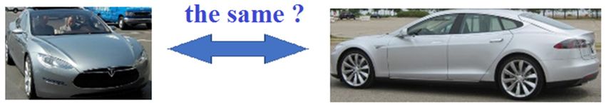
Appl. Sci. 2021, 11, 5863                                                                                                   7 of 14

                            where r is the image-pair similarity score. This score is responsible for ensuring that the
                            positive image is more similar to the “average” one than the negative image. In our solution,
                            we take positive images from the given class of model-view and negative images from
                            another class of model-view. DeepRanking metric D is the Euclidean distance between
                            two feature vectors. λ is a regularization parameter that controls the margin of the learned
                            ranker to improve its generalization [8]. The g is a gap parameter that regularizes the
                            gap between the distance of the two image pairs: (pi , pi + ) and (pi , pi − ). Function f (p)
                            is the image embedding function. W is the parameters of the embedding function. It is
                            considered to be one of the best neural network architectures for image matching (based on
                            published results). Hence, we selected DeepRanking to obtain image-pair similarity scores.

                            3.5. Key-Point Feature Matching
                                 In addition to DeepRanking, we use an alternative processing stream to obtain image
                            pair similarity. Hand-crafted features (keypoints and their local descriptors) are extracted
                            from the images. We apply the standard SIFT approach. Other schemes which are com-
                            putationally more efficient and of similar quality such as SURF or ORB could also be
                            used [10,11]. According to [11], SIFT gives the best image matching in most of the tested
                            cases. In real-time applications, binary descriptors would be preferred [12].

                            3.6. BSS Scoring for Image Sets
                                   Assume that similarity scores pi, j are provided for every image pair (i, j), I = 1, 2, . . . ,
                            n and j = 1, 2, . . . , m. They are collected in a similarity matrix P = [pij ], where pij = similarity
                            (Ii, Ij). The error index (or dissimilarity score) for two image sets is defined as [9]:
                                                                                  !                         !
                                                              1                        1
                                                              m ∑     ∑ peij − n + n ∑ ∑ pij − m
                                                     EI (P) =                                                                   (2)
                                                                    i j                    j i

                                Two normalized versions of the matrix P are computed. In the first case, in every row
                            of matrix P the maximum entry is found and all entries in a given row are divided by this
                            maximum value:

                            •   every row i of P is scaled: Pe = Norm( P), such that ∀i max j e
                                                                                              aij = 1
                                 In the second case, the maxima are found independently in every column of P and the
                            entries in every column are divided by their corresponding maximum value:

                            •    every column j is scaled: Pe = NormCol ( P), such that ∀ j maxi e
                                                                                                 aij = 1 .
                                  Therefore, in an ideal case of two set matching, the first normalized matrix will have
                            in every row only one nonzero entry equal to 1, while the second matrix will have a single
                            entry 1 and all other entries in every column a 0. By subtracting from the sum of all row- or
                            column-normalized elements the number of columns and rows, appropriately, the nonzero
                            result will represent an average distance score between two images, while the one-valued
                            entries will verify whether the checked set contains a single car model and all the required
                            different views.
                                  The BSS-based similarity score for two sets is obtained in two different modes—the
                            image-to-image comparison mode and the ROI-to-ROI comparison mode (Figure 5). In
                            the first case, a feature vector (DeepRanking embeddings or SIFT descriptors) is calculated
                            for every (masked) image in every set. The similarity matrix P is of size 4 × 4, where
                            every entry represents the similarity score for the features of a pair of images (Figure 5a).
                            In the second mode, every image from a set of four images is represented by five ROIs
                            and their feature vectors (DeepRanking embeddings or SIFT descriptors) are given. Thus,
                            we calculate the BSS error index (EI(P)) for a 20 × 20 similarity matrix P, where the first
                            set ROIs play the role of the “BSS sources”, while the second set ROIs are the estimated
                            “separated signals” (Figure 5b).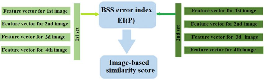
Appl. Sci. 2021, 11, 5863 8 of 14
Appl. Sci. 2021, 11, x FOR PEER REVIEW 8 of 14
(a)
(b)
Figure 5.
Figure 5. The
Thescheme
schemeofof“BSS
“BSSscoring” forfor
scoring” calculating thethe
calculating similarity of two
similarity image
of two sets:sets:
image (a) the
(a)“im-
the
age-to-image” comparison
“image-to-image” mode,
comparison andand
mode, (b) (b)
thethe
“ROI-to-ROI”
“ROI-to-ROI”comparison
comparison mode.
mode.
3.7. Car Model Classifier
Car
Car model
modelclassifier
classifierisisneeded
neededto to
boost the the
boost accuracy of the
accuracy ofimage set comparison
the image score.
set comparison
We have
score. Weahave
closed list oflist
a closed theofmodels (classes)
the models available
(classes) for the
available for problem. TheThe
the problem. classifier is
classifier
defined as as
is defined a pretrained
a pretrainedneural network
neural network based on the
based Inception
on the V3 [5]
Inception V3architecture withwith
[5] architecture 197
classes (196(196
197 classes cars cars
and andone “other” class).
one “other” class).
cm11 . . .. ... . cm
1 197
. .
. .
. . (3)
. .cm
. im ..
(3)
.
For each image, I (I = 1, …,cm 41 its
4), . cm4197
. . similarity .scores with respect to the 197 models are
obtained. The highest scored model is selected as an image
For each image, I (I = 1, . . . , 4), its similarity scores with vote. The class
respect to thewith the ma-
197 models
jority of votes given by the images in a set is selected as the set’s winner [23].
are obtained. The highest scored model is selected as an image vote. The class with the
majority of votes given by= ( images
the , , in, a set, is selected =
where asargmax
the set’s winner [23].
(4)
CM = (m1 , m2 , m3 , m4 ), where mi = argmaxcmij (4)
j
3.8. Car Type Classifier
TheType
3.8. Car purpose of the car type classifier is to determine the general type of the car pre-
Classifier
sented
The purpose ofofthe
in all images a set.
carThere
type are eight types
classifier is to distinguished:
determine theVan, Sedan,
general Coupe,
type of theSUV,
car
presented in all images of a set. There are eight types distinguished: Van, Sedan, “other”
Cabriolet, Hatchback, Combi, and Pickup, with four views for each type, and the Coupe,
class Cabriolet,
SUV, for non-recognized
Hatchback, types. Thisand
Combi, classifier
Pickup, is also
withbased on thefor
four views InceptionV3
each type, [5]
anddeep
the
neural network. For each image in a set, the highest scored type is selected
“other” class for non-recognized types. This classifier is also based on the InceptionV3 as the image[5]
vote. neural
deep The class with the
network. Formajority of votes
each image in agiven
set, thebyhighest
the images in type
scored a set is
is selected
selected as
as the
the
set’s winner
image [23].class with the majority of votes given by the images in a set is selected as
vote. The
the set’s winner [23]. .. . . .
ct11. . .. . . ct. 141
. . . (5)
.. . . . .
(5)
. ctit .
ct41. . . . . ct441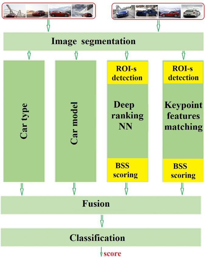
Appl. Sci. 2021, 11, 5863                                                                                                     9 of 14

                                                                                                                     !
                                                 CT = ( f t1 , f t2 , f t3 , f t4 ) , where f ti = type(argmaxctij               (6)
                                                                                                           j

                                 Remark: type () gets the type index from the view-type class identifier.

                            3.9. Fusion
                                 Fusion is the layer where results from all streams are combined into one vector v of all
                            available scores. This vector is classified in the final classification step:

                                         v = CT1 , CT2 , CM1 , CM2 ,         i − to − i, ROI − to − ROI               (7)

                            where:
                            •    CTi is the indicator vector for car type for the i-th set,
                            •    CMi is the car model indicator vector for the i-th set,
                            •    i-to-i is the value of the two-set similarity score based on the BSS error index obtained
                                 in image mode, and
                            •    ROI-to-ROI is the value of the two-set similarity score based on the BSS error index
                                 obtained in ROI mode.

                            3.10. Final Classification
                                 Final classification gives the estimated similarity score of both image sets provided
                            at the system’s input. This step is implemented as a feedforward neural network with
                            four fully connected layers (see a detail description of layers in Table 2). The fused vector
                            (Equation (7)) is a rather short one. Thus, the neural network can have a simple architecture.
                            The final score is in the interval 0–1, where 0 represents “different” objects, while 1 means
                            the same object exists in both sets.

                            Table 2. Architecture of the final classifier in our solution.

                                     Layer Number                       Type of the Layer                      Output Size
                                             1                                Dense                                       6
                                             2                         Batch normalization                                6
                                             3                                Dense                                      18
                                             4                         Batch normalization                               18
                                             5                                Dense                                      18
                                             6                         Batch normalization                               18
                                             7                                Dense                                       2

                            4. The Base Solution
                                 In the experiments, we are going to compare the current approach with an earlier
                            developed base solution [24]. Several modifications have been made—they are summarized
                            as follows:
                            •    Now we calculate the BSS-based similarity score to resolve the unknown permutation
                                 of views in two sets.
                            •    The base system has no car model stream.
                            •    Additionally, to the “image-to-image-mode”, given in the baseline, in the presented
                                 approach the similarity score in the “ROI-to-ROI” mode is also computed.
                            •    The final classification network has been simplified. Compare the current classifier
                                 network (Table 2) with such a network in the base solution (Table 3).
                                 Although the two new results are fused, due to the use of the explicit BSS score the
                            fused vector is now of the same length as before (18 elements). It also turned out that the
                            size of the final classification network can be much lower than in the baseline.
Appl. Sci. 2021, 11, 5863 10 of 14
Table 3. Architecture of the final classifier for the base solution.
Layer Number Type of the Layer Output Size
1 Dense 64
2 Batch Normalization 64
3 Dense 128
4 Batch Normalization 128
5 Dense 196
6 Batch Normalization 196
7 Dense 128
8 Batch Normalization 128
9 Dense 2
5. Results
For an experimental evaluation, the Stanford Cars dataset [25] was used. We fixed the
number of images in every image set to four. The order of views in the set is not relevant.
We assumed that each proper set has four views: front, side, front-side, and back-side.
Obviously, the approach is view-independent and in other applications any other number
of views can be set. This doesn’t mean that with different views we can get the same
quality of results. The choice of a specific kind of view depends on the user’s decision
and their experience. From a technical and methodological point of view, our solution is
independent of the selection of object views. Our dataset has less accurate data of back
view images, so we decided to skip this view. Hence, the dataset is labeled by 4 views, 9
car types, and 197 car models. Both types of object-related label contain the class other for
images which are not matched with the basic labels.
We conducted several experiments with this dataset and different settings of the
system, and produced much improved results compared with the earlier base solution. The
assumptions for the experiments are described in Table 4. With the same dataset we used,
alternatively, DeepRanking- or SIFT-based features, and turned on or off an additional
stream for car model classification. The dataset was split into learning (70%) and test
parts (30%), and every experiment was repeated 10 times with different dataset splits. In
Table 4, the average accuracy rates of different configurations of the proposed solution
and the base solution are presented. By “accuracy”, we mean the “genuine acceptance
rate” (GAR) of a recognition system when “false acceptance rate” (FAR) is kept at 3%. The
summarized accuracy of set-similarity recognition was increased from 50.2%, for the best
baseline setting, to 67.7% for the best option of proposed approach. The best architecture
appeared to include the (additional) car model classification stream and the DeepRanking
net for feature extraction (instead of the SIFT descriptor).
Table 4. Average accuracy of the similarity of two image sets.
Model Accuracy
Base solution (DeepRanking + Euclidean distance) [24] 50.2%
Proposed with DeepRanking and BSS score, without car model stream 62.1%
Proposed with DeepRanking and BSS score and car model stream 67.7%
Proposed with SIFT and BSS score, without car model stream 61.6%
Proposed with SIFT and BSS score and car model stream 64.4%
As we can clearly see in Table 4, the use of an explicit BSS error index as a measure of
permutation-independent distance between two image sets and the additional car model
classification stream allow for a significant improvement in the set similarity classification
accuracy. For image feature extraction, it is more advantageous to use the DeepRanking
approach than the classic SIFT descriptor.
At first glance, the accuracy value of 67.7% seems to be a relatively worse result.
However, the considered problem is rather hard to solve. Let us illustrate the results in
more detail, by considering three different set-versus-set situations (Table 5):Appl. Sci. 2021, 11, x FOR PEER REVIEW 11 of 14
Appl. Sci. 2021, 11, x FOR PEER REVIEW 11 of 14
Appl.Sci.
Appl. Sci.2021,
2021,11,
11,5863
x FOR PEER REVIEW 11 of 14
11 of 14
At first glance, the accuracy value of 67.7% seems to be a relatively worse result.
At first
However, glance,
theglance, the accuracy
considered value
problemvalue of 67.7%
is rather hard toseems to be us
solve. a relatively worse result.
At first the accuracy of 67.7% seems to Let illustrate worse
be a relatively the results in
result.
However,
more the
detail, byconsidered
considering problem
three is rather
different hard to solve.
set-versus-set Let us
situationsillustrate
(Table the
5): results in
However, the considered problem is rather hard to solve. Let us illustrate the results in
more detail, by considering three different set-versus-set situations (Table 5):
1.
1. the
more same
detail,
the same bycar model
model and
considering
car the
andthreethe same views
different
same views in
in both
both sets
sets(Figure
set-versus-set (Figure6),
situations6),(Table 5):
1.
2.
2. the
the
the same
same
same car
car
car model
model
model and
but
but the same views
inconsistent
inconsistent in (Figure
views
views both sets
(Figure (Figure
7),
7), and
and 6),
1. the same car model and the same views in both sets (Figure 6),
2.
3. the same car
3. different car models
model but inconsistent views (Figure 7), and
2. the same car
different car models (Figure
model but(Figure 8).
8).
inconsistent views (Figure 7), and
3. different car models (Figure 8).
3. different car models (Figure 8).
Table 5. Averagefinal
final set-similarityscores
scores fordifferent
different situations.
Table5.5.Average
Table Average finalset-similarity
set-similarity scoresfor
for differentsituations.
situations.
Table 5. Average final set-similarity scores for different
Base situations.
Approach
Case
Case Base Approach
Base Approach[24] Proposed
Proposed Should
ShouldBeBe
Case [24]
Base Approach Proposed Should Be
Same car modelCase
and same view 0.708
[24] 0.821
Proposed 1.0 Be
Should
Same
Same car
carcar model
model and same
but different view
views 0.708
[24]
0.531 0.821
0.597 1.0
~0.5
Same model and same view 0.708 0.821 1.0
Same
Samecar model
car model
Different but
car different
and views
same view
model 0.531
0.708
0.208 0.597
0.821
0.180 ~0.5
1.0
0.0
Same car model but different views 0.531 0.597 ~0.5
Different car model
Same car model but different views 0.208
0.531 0.180
0.597 0.0
~0.5
Different car model 0.208 0.180 0.0
Different car model 0.208 0.180 0.0
Figure6.6.Example
Figure Exampleof
ofsituation:
situation:the
thesame
samecar
carmodel
modeland
andsame
sameview
viewtypes.
types.
Figure 6. Example of situation: the same car model and same view types.
Figure 6. Example of situation: the same car model and same view types.
Figure 7. Example of situation: the same car model but different view types.
Figure7.7.Example
Example ofsituation:
situation: the same
same carmodel
model butdifferent
different viewtypes.
types.
Figure 7. Example of
Figure of situation: the
the same car
car model but
but differentview
view types.
Figure 8. Example of situation: different car model.
Figure 8. Example of situation: different car model.
Figure8.
Figure 8. Example
Example of
of situation:
situation: different
different car
car model.
model.
In comparison with the base solution, the discrimination ability of the similarity score
In comparison
is much with the
improved—the base solution,
discrepancy the discrimination
between different- andability of theaverage
same-set similarity score
score is
In comparison
In comparison withthe
with the base solution,
base solution, the discrimination
the discrimination ability
ability ofthe
of thesimilarity
similarity score
score
is much
raised improved—the
from 0.500 discrepancy
(=0.708–0.208) to between
0.641 different-
(=0.821–0.180). and same-set
However, the average
score is score
still is
sensi-
is much
is much improved—the
improved—the discrepancy
discrepancy between
between different-
different- and
and same-set
same-set average
average score
score isis
raised from
tive tofrom 0.500
even0.500
small (=0.708–0.208)
changes of the toviewpoint
0.641 (=0.821–0.180). However,
direction, However,
even when the score is still sensi-
raised
raised from 0.500 (=0.708–0.208)
(=0.708–0.208) toto0.641
0.641 (=0.821–0.180).
(=0.821–0.180). However, theonly
the one
score
score image-pair
is still
is still in
sensi-
sensitive
tive to even small changes of the viewpoint direction, even when only one image-pair in
to even
tive smallsmall
to even changes of theof
changes viewpoint direction,
the viewpoint even when
direction, evenonly
whenone image-pair
only in the set
one image-pair inAppl. Sci. 2021, 11, 5863 12 of 14
Appl. Sci. 2021, 11, x FOR PEER REVIEW 12 of 14
isthe
affected
set is by such aby
affected situation. An image-pair
such a situation. similarity score
An image-pair of around
similarity score0.5
ofmay result
around 0.5from
may
obviously different views or from a visible change of the viewpoint direction,
result from obviously different views or from a visible change of the viewpoint direction, but within
the
butsame
withinview
thetype
same (see Figure
view type9). Although
(see Figure 9).every individual
Although everyscore only partly
individual scorecontributes
only partly
tocontributes
the final set-similarity
to the final set-similarity score, one low score alone affects the overall score.
score, one low score alone affects the overall set-related set-re-
For thescore.
lated final For
decision, wedecision,
the final applied awe conservative threshold that
applied a conservative corresponds
threshold to a false
that corresponds
acceptance rate of 3% (in
to a false acceptance rateevery
of 3%configuration). The focus on
(in every configuration). Thefalse acceptance
focus on false avoidance
acceptance
leads to a relatively low accuracy ratio (67.7%). The overall score
avoidance leads to a relatively low accuracy ratio (67.7%). The overall score isis obviously dependent
obviously
on the quality
dependent onof
theindividual
quality ofdata analysis
individual streams.
data Letstreams.
analysis us observe theobserve
Let us averagethe accuracy
average
(GAR at 3%(GAR
accuracy FAR)atof3%some
FAR)individual
of somestreams andstreams
individual the image segmentation
and step obtainedstep
the image segmentation in
the experiments:
obtained in the experiments:
• accuracy of the single-image car type classification stream was 75.1%,
• accuracy of the single-image car type classification stream was 75.1%,
• single-image car model classification accuracy was 66.3%, and
• single-image car model classification accuracy was 66.3%, and
• accuracy of the semantic segmentation (a subjective evaluation of the proper detection
• accuracy of the semantic segmentation (a subjective evaluation of the proper detec-
of the car mask region) was 89.7%.
tion of the car mask region) was 89.7%.
Figure9.9.Illustration
Figure Illustrationofofcar
carmask
maskdetection
detectionininsingle-car
single-carimage.
image.
ItItisisclearly
clearlyvisible
visiblethat
thataaproper
properdetection
detectionofofthetheobject’s
object’sROIROIininthe
theimage
imageallows
allowsforfor
the improvement
the improvement of of the classification accuracy of the entire approach. Let us
classification accuracy of the entire approach. Let us illustrate illustrate this
factfact
this with an example.
with an example.In Figure 9, two
In Figure different
9, two carscars
different of the of same
the sametypetype
and and
model are com-
model are
pared twotwo
compared times—by
times—by matching
matchingentire images
entire images(the leftleft
(the pair of images)
pair of images) and by by
and matching
matching the
previously
the previously detected object
detected ROIs
object (the(the
ROIs right pairpair
right of images).
of images).We Weexpect thatthat
expect the proper
the propersim-
ilarity score
similarity forfor
score thethe
same
same view of of
view thethe
same
samecarcar
model
model should
should beberather high
rather high(>0.5). ForFor
(>0.5). the
the
set set of images
of images on the
on the left,left, we agot
we got lowa low similarity
similarity scorescore of 0.190
of 0.190 (the same
(the same car model
car model under
under a slightly
a slightly different
different view butview but awith
with verya different
very different background),
background), while while
for thefor theimage
ROI ROI
image
pair on pair theonright
the right sidescore
side the the score was 0.492
was 0.492 (where(where the background
the background waswas eliminated
eliminated in
in ROI
ROI masked
masked images).
images).
6.6.Limitations
Limitations
Our
Ourapproach
approachand proposed
and proposedsolution have
solution several
have limitations.
several The The
limitations. first first
beingbeing
that our
that
approach cannot be applied to any image content; the proposed solution is
our approach cannot be applied to any image content; the proposed solution is valid only valid only for
images with with
for images a single foreground
a single object.object.
foreground The second limitation
The second is that we
limitation are we
is that matching object
are matching
views, but we do not make view registration (i.e., view normalization) by
object views, but we do not make view registration (i.e., view normalization) by trans- transforming
image
formingcontent.
image If an image
content. pair
If an shares
image pairthe samethe
shares type of object
same type ofview
objectbut thebut
view viewpoints
the view-
differ too much, the similarity score may be lower than needed. Two other limitations are
points differ too much, the similarity score may be lower than needed. Two other limita-
of technical nature, as we require the same granularity of labels in the dataset and require
tions are of technical nature, as we require the same granularity of labels in the dataset
the same number of images in both sets. All of these limitations can be considered in future
and require the same number of images in both sets. All of these limitations can be con-
research and some of them will be relatively easily addressed.
sidered in future research and some of them will be relatively easily addressed.
7. Conclusions
7. Conclusions
An approach to image-set similarity evaluation was proposed based on the fusion
An approach
of several to image-set
image processing andsimilarity evaluation
classification was The
streams. proposed based
achieved on the fusionre-
experimental of
several image processing and classification streams. The achieved experimental resultsAppl. Sci. 2021, 11, 5863 13 of 14
sults confirmed that the new solution’s steps, as proposed in this paper, give a visible
improvement of the previous baseline approach. They include an additional car model
classification stream and the use of an explicit BSS-based permutation-independent score
of image sets. Once more, the advantage of using a DeepRanking network with its triplet
loss function for image feature extraction was confirmed. The evaluation of image-pair
similarity results obtained by the DeepRanking stream has demonstrated its strengths
over a classic stream based on SIFT features. Another conclusion from this work is the
importance of using application-dependent classification streams (e.g., the car type and
car model-and-view information), representing semantic content information and not
solely application-independent streams for image similarity evaluation. The car model
classification stream has improved our results by another few points.
8. Discussion
We have shown that a multi-stream fusion of application-independent and seman-
tic streams is a prospective approach to image-set similarity evaluation. Our approach
gives strong advice on the design of a generalized framework. The design of application-
independent streams (e.g., image similarity scoring) should preferably use machine learning-
based features instead of hand-crafted features, however, the use of smart distance metrics
(e.g., BSS error index) is extremely important. A correct selection of semantic processing
streams is also strongly recommended. In the context of using machine learning method-
ology, the required semantic data sets are much easier to obtain and label than the data
needed for universal model creation.
In future research, we would like to generalize the approach by adopting it to other
object categories. Explainable AI (XAI) techniques are also of interest to explain the
contribution of particular processing streams and steps to the overall result. XAI techniques
allow us to answer an important set of questions: not only whether something is similar,
but also why it is similar. This would enable a further generalization of our approach,
which could be applied not only in image set comparison, but in other pattern sets as well
(e.g., text or multi-modal sets of sources).
Author Contributions: Conceptualization, P.P. and W.K.; methodology, P.P. and W.K.; software, P.P.;
validation, P.P.; formal analysis, P.P.; investigation, P.P. and W.K.; resources, P.P. and W.K.; data
curation, P.P.; writing—original draft preparation, P.P. and W.K.; writing—review and editing, W.K.;
visualization, P.P. and W.K.; supervision, W.K. All authors have read and agreed to the published
version of the manuscript.
Funding: This research received no external funding.
Institutional Review Board Statement: Not applicable.
Informed Consent Statement: Not applicable.
Data Availability Statement: http://ai.stanford.edu/~jkrause/cars/car_dataset (accessed on 23
June 2021).
Conflicts of Interest: The authors declare no conflict of interest.
References
1. Gesù, V.; Starovoitov, V. Distance-based functions for image comparison. Pattern Recognit. Lett. 1999, 20, 207–214. [CrossRef]
2. Gaillard, M.; Egyed-Zsigmond, E. Large scale reverse image search: A method comparison for almost identical image retrieval.
In Proceedings of the INFORSID, Toulouse, France, 31 May 2017; p. 127. Available online: https://hal.archives-ouvertes.fr/hal-
01591756 (accessed on 23 June 2021).
3. Krause, J.; Stark, M.; Deng, J.; Fei-Fei, L. 3D Object Representations for fine-grained categorization. In Proceedings of the 2013
IEEE International Conference on Computer Vision Workshops, ICCVW 2013, Sydney, Australia, 1–8 December 2013; pp. 554–561.
[CrossRef]
4. Uijlings, J.R.R.; Van De Sande, K.E.A.; Gevers, T.; Smeulders, A.W.M. Selective search for object recognition. Int. J. Comput. Vis.
2013, 104, 154–171. [CrossRef]You can also read