Exact Probability Landscapes of Stochastic Phenotype Switching in Feed-Forward Loops: Phase Diagrams of Multimodality
←
→
Page content transcription
If your browser does not render page correctly, please read the page content below
ORIGINAL RESEARCH
                                                                                                                                                     published: 08 July 2021
                                                                                                                                           doi: 10.3389/fgene.2021.645640

                                              Exact Probability Landscapes of
                                              Stochastic Phenotype Switching in
                                              Feed-Forward Loops: Phase
                                              Diagrams of Multimodality
                                              Anna Terebus 1,2† , Farid Manuchehrfar 1† , Youfang Cao 1,3 and Jie Liang 1*
                                              1
                                                Center for Bioinformatics and Quantitative Biology, Richard and Loan Hill Department of Bioengineering, University of Illinois
                                              at Chicago, Chicago, IL, United States, 2 Constellation, Baltimore, MD, United States, 3 Merck & Co., Inc., Kenilworth, NJ,
                                              United States

                                              Feed-forward loops (FFLs) are among the most ubiquitously found motifs of reaction
                                              networks in nature. However, little is known about their stochastic behavior and the variety
                           Edited by:
                                              of network phenotypes they can exhibit. In this study, we provide full characterizations
                           Chunhe Li,         of the properties of stochastic multimodality of FFLs, and how switching between
                Fudan University, China       different network phenotypes are controlled. We have computed the exact steady-state
                       Reviewed by:           probability landscapes of all eight types of coherent and incoherent FFLs using the
                            Yang Cao,
          Virginia Tech, United States        finite-butter Accurate Chemical Master Equation (ACME) algorithm, and quantified
                       Davit Potoyan,         the exact topological features of their high-dimensional probability landscapes using
  Iowa State University, United States
                                              persistent homology. Through analysis of the degree of multimodality for each of a set of
                   *Correspondence:
                              Jie Liang
                                              10,812 probability landscapes, where each landscape resides over 105 –106 microstates,
                        jliang@uic.edu        we have constructed comprehensive phase diagrams of all relevant behavior of FFL
     † These   authors have contributed
                                              multimodality over broad ranges of input and regulation intensities, as well as different
                    equally to this work      regimes of promoter binding dynamics. In addition, we have quantified the topological
                                              sensitivity of the multimodality of the landscapes to regulation intensities. Our results
                    Specialty section:
                                              show that with slow binding and unbinding dynamics of transcription factor to promoter,
          This article was submitted to
                        Biology Archive,      FFLs exhibit strong stochastic behavior that is very different from what would be
                a section of the journal      inferred from deterministic models. In addition, input intensity play major roles in the
                   Frontiers in Genetics
                                              phenotypes of FFLs: At weak input intensity, FFL exhibit monomodality, but strong
       Received: 23 December 2020
           Accepted: 26 April 2021
                                              input intensity may result in up to 6 stable phenotypes. Furthermore, we found that
           Published: 08 July 2021            gene duplication can enlarge stable regions of specific multimodalities and enrich the
                             Citation:        phenotypic diversity of FFL networks, providing means for cells toward better adaptation
    Terebus A, Manuchehrfar F, Cao Y
                                              to changing environment. Our results are directly applicable to analysis of behavior of
  and Liang J (2021) Exact Probability
 Landscapes of Stochastic Phenotype           FFLs in biological processes such as stem cell differentiation and for design of synthetic
   Switching in Feed-Forward Loops:           networks when certain phenotypic behavior is desired.
     Phase Diagrams of Multimodality.
             Front. Genet. 12:645640.         Keywords: systems biology, feed forward loop, gene regulatory network, network motif, stochastic reaction
     doi: 10.3389/fgene.2021.645640           network, persistent homology, ACME algorithm

Frontiers in Genetics | www.frontiersin.org                                           1                                               July 2021 | Volume 12 | Article 645640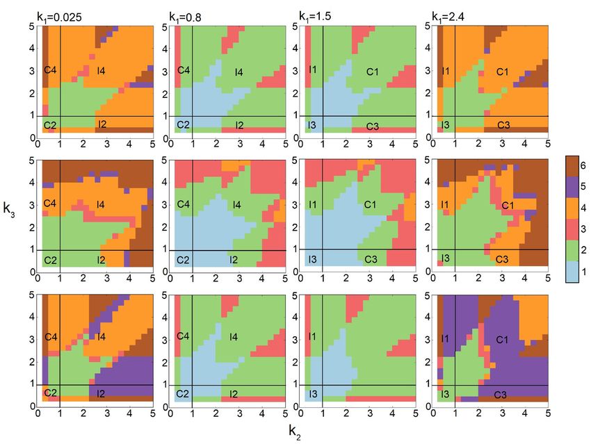
Terebus et al.                                                                                        Stochastic Multimodality of Feed-Forward Loops

1. INTRODUCTION                                                            FFLs is not well-characterized: Basic properties such as the
                                                                           number of different phenotypes FFLs are capable of exhibiting,
Cells with the same genetic make-ups can exhibit a variety of              the conditions required for their emergency, their relative
different behavior. They can also switch between these different           prominence, and the sensitivity of different phenotypes to
phenotypes stochastically. This phenomenon has been observed               perturbations are not known.
in bacteria, yeast, and mammals such as neural cells (Acar                    Our stochastic FFL models are based on processes of
et al., 2005; Choi et al., 2008; Guo and Li, 2009; Gupta et al.,           Stochastic Chemical Kinetics (SCK), which provides a general
2011). The ability to exhibit multiple phenotypes and switching            framework for understanding the stochastic behavior of reaction
between them is the foundation of cellular fate decision (Schultz          networks. Quantitative SCK modeling can uncover different
et al., 2007; Cao et al., 2010; Ye et al., 2019), stem cell                network phenotypes, the conditions for their occurrence, and
differentiation (Feng and Wang, 2012; Papatsenko et al., 2015;             the nature of the prominence of the stability peaks. However,
Zhang et al., 2019), and tumor formation (Huang et al., 2009;              analysis of stochastic networks is challenging. First, models
Shiraishi et al., 2010).                                                   based on stochastic differential equations such as Fokker–
    Cells exhibiting different phenotypes have different patterns          Planck and Lagenvin models may be inadequate due to their
of gene expression. Single-cell studies demonstrated that isogenic         Gaussian approximations. This is further compounded by the
cells can exhibit different modes of gene expression (Shalek et al.,       limited number of simulation trajectories that can be generated.
2013), indicating that distinct phenotypes are encoded in the              These difficulties are reflected in the reported failure of a
wiring of the genetic regulatory networks (Liang and Qian, 2010).          Fokker–Planck model in accounting for multimodality in the
This phenomenon of epigenetic control of bimodality in gene                simple network model of single self-regulating gene at certain
expression by network architecture is well-known and has been              reaction rates (Duncan et al., 2015). Second, the widely used
extensively studied in earlier works of phage-lambda (Arkin et al.,        Stochastic Simulation Algorithm (Gillespie simulations) can
1998; Ptashne, 2004; Zhu et al., 2004a,b; Cao et al., 2010).               generate SCK trajectories (Gillespie, 1977), but are challenged
    Understanding multimodality in gene regulatory networks                in capturing rare events and in computing efficiency. There
and its control mechanism can provide valuable insight into                are also difficulties in assessing convergency and in estimating
how different cellular phenotypes arises and how cellular                  computational errors (Cao and Liang, 2013). Third, even if
programming and reprogramming proceed (Lu et al., 2007).                   the probabilistic landscape can be accurately reconstructed
Much of current knowledge of multimodality is derived                      with acceptable accuracy, detecting topological features such as
from analysis of networks with feedback loops or cooperative               peaks in high-dimensional probability landscapes and assessing
interactions (Siegal-Gaskins et al., 2009). However, recent studies        their objectively prominence at large-scale remains an unsolved
suggest that multimodality and phenotype switching can also                problem.
arise from slow promoter binding, which may result in distinct                To characterize the stochastic behavior of FFLs using models
protein expression levels of long durations (Feng and Wang,                based on SCK processes, our approach is to solve the underlying
2012; Thomas et al., 2014; Chen et al., 2015; Duncan et al., 2015;         discrete Chemical Master Equation (dCME) using the ACME
Terebus et al., 2019). Nevertheless, the nature and extent of this         (Accurate Chemical Master Equation) algorithm (Cao et al.,
type of bimodality is not well-understood.                                 2016a,b), and to obtain the exact probability landscapes of all 8
    In this work, we study the network modules of feed-                    varieties of FFLs.
forward loops (FFLs) and characterize the stochastic nature                   Aided by the computational efficiency of ACME, we are
of their multimodalities. FFLs are one of the most prevalent               able to explore the behavior FFLs under broad conditions
three-node network motifs in nature (Alon, 2006) and play                  of synthesis, degradation, binding, and unbinding rates of
important regulatory roles (Lee et al., 2002; Shen-Orr et al.,             transcription factors genes binding. Furthermore, we analyze the
2002; Boyer et al., 2005; Mangan et al., 2006; Tsang et al., 2007;         topological features of the exactly constructed high-dimensional
Ma et al., 2009; Sorrells and Johnson, 2015). They appear in               probability landscapes using persistent homology, so the number
stem cell pluripotency networks (Boyer et al., 2005; Papatsenko            of probability peaks and the prominence measured by their
et al., 2015; Sorrells and Johnson, 2015), microRNA regulation             persistence are quantified objectively. These techniques allow
networks (Tsang et al., 2007; Re et al., 2009; Ivey and Srivastava,        us to examine details of the number of possible phenotypic
2010), and cancer networks (Re et al., 2009). The behavior of FFLs         states at different conditions, as well as the ranges of conditions
has been studied extensively using deterministic ODE models.               enabling phenotypic switching. With broad exploration of the
These studies revealed important functions of FFLs in signal               model parameter space, we are able to construct detailed phase
processing, including sign-sensitive acceleration and delay pulse          diagrams of multimodalities under different conditions.
generation functions, and increased cooperativity (Mangan and                 Our results reveal how FFL network behaves differently under
Alon, 2003; Ma et al., 2009). FFLs are also found to be capable            varying strengths of regulations intensities and the input. In
of maintaining robust adaptation (François and Siggia, 2008; Ma            addition, we characterize quantitatively the effects of duplication
et al., 2009) and detecting “fold-changes” (Goentoro et al., 2009).        of genes in the FFL network modules. We show gene duplication
    However, analysis based on ODEs is limited in its ability              can significantly affect the diversity of multimodality, and can
to characterize probabilistic events, as they do not capture               enlarge monomodal regions so FFLs can have robust phenotypes.
bimodality in gene expression that arises from slow promoter               The results we obtained can be useful for analysis of phenotypic
binding (Vellela and Qian, 2009). The stochastic behavior of               switching in biological networks containing the FFL modules.

Frontiers in Genetics | www.frontiersin.org                            2                                       July 2021 | Volume 12 | Article 645640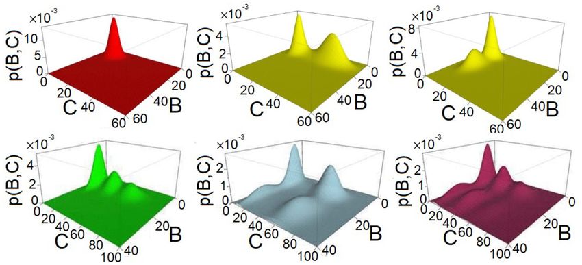
Terebus et al. Stochastic Multimodality of Feed-Forward Loops
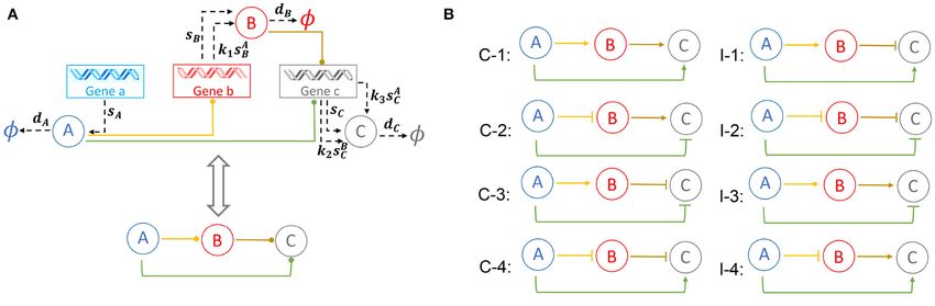
FIGURE 1 | Representation and the types of feed-forward loop (FFL) network: (A) General wiring and corresponding 3-node schematic representation of an FFL
module containing three genes a, b, and c expressing three proteins A, B, and C. Protein A regulates the expressions of genes b and c through binding to their
promoters. Protein B regulates the expression of gene c through promoter binding. (B) The FFL modules can be classified into eight different types.
Coherent/incoherent FFLs are on the left/right, respectively.
They can also be used for construction of synthetic networks with Upon binding protein A, bA expresses protein B at a rate k1 -fold
the goal of generating certain desired phenotypic behavior. over the basal rate of sB .
The biochemical reactions of our FFL model are summarized
below:
2. MODELS AND METHODS
rbA fbA
2.1. Architecture and Types of b + A → bA; bA → b + A;
Feed-Forward Loop Network Modules
2.1.1. Overview rcA fcA
c + A → cA; cA → c + A;
FFLs consists of three nodes representing three genes, each
expresses a different protein product (Figure 1A). An FFL
rcB fcB
regulates the network output from the left input node toward c + B → cB; cB → c + B;
the right output node via two paths; the direct path from the
left node to the right node, and the indirect path from the left
sA dA
to the right node via an intermediate buffer node. As each of the a → a + A; A → ∅;
three regulations can be either up- or downregulation, there are
altogether 23 = 8 types of FFL. sB sB ∗k1 dB =1
b → b + B; bA → bA + B; B → ∅;
2.1.2. Network Architecture
Specifically, we denote the three genes of an FFL module as a, b, sC sC ∗k2 sC ∗k3 dC
c → c + C; cB → cB + C; cA → cA + C; C → ∅.
and c, which expresses protein products A, B, and C at constant
synthesis rate of sA , sB , and sC , respectively (Figure 1A). Proteins Here, we set rbA = rcA = rcB = 0.005 s−1 , fbA = fcA = fcB = 0.1 s−1 ,
A, B, and C are degraded at rate dA , dB , and dC , respectively. dA = dB = dC = 1 s−1 , and sA = sB = sC = 10 s−1 . All reaction
Both proteins A and B function as transcription factors and can rate constants are of the unit s−1 , while coefficients k1 , k2 , and
bind competitively to the promoter of gene c and regulates its k3 are ratio of reaction rates and therefore unitless. The ratios
expression. As the promoter of gene c can bind to either protein k1 , k2 , and k3 can take different values so the network represents
A or B, but not both, this type of regulation is known as the “OR” different types of FFLs.
gate. In addition, protein A can bind to the promoter of gene b
and regulate its expression. Specifically, protein A can bind to 2.1.3. Types of FFL Modules
the promoter of gene c at rate rcA to form complex cA, which Depending on the nature of the regulations, namely, whether
dissociates at rate fcA . cA expresses protein C at a rate k3 -fold over each of regulation intensities k1 , k2 , and k3 is ≥ 1 (activating)
the basal rate of sC . Similarly, protein B can bind to the promoter or < 1 (inhibiting), there are 23 = 8 types of FFLs. These
of gene c at rate rcB to form complex cB, which dissociates at rate FFLs are classified into two classes, the coherent FFLs and the
fcB . cB expresses protein C at a rate k2 -fold over the basal rate of incoherent FFLs (Figure 1B) (Alon, 2006). A FFL is termed
sC . Furthermore, protein A binds to the promoter of gene b at rate coherent (C1 , C2 , C3 , C4 in Figure 1B), if the direct effect of
rbA to form gene–protein complex bA, which dissociate at rate fbA . protein A on the gene c has the same sign (positive or negative)
Frontiers in Genetics | www.frontiersin.org 3 July 2021 | Volume 12 | Article 645640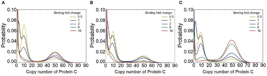
Terebus et al.                                                                                                          Stochastic Multimodality of Feed-Forward Loops

TABLE 1 | Parameter ranges for eight types of feed-forward loop (FFL) model.            = {x(t)|t ∈ [0, ∞)}. In this study, the size of the state space
                                                                                       is || = 657, 900 when genes b and c are single-copy, and
FFL type                k1 range              k2 range               k3 range
                                                                                       || = 686, 052 and 1, 289, 656 when there are two copies of gene
C1                      (1.0 3.0]              (1.0 5.0]              (1.0 5.0]        b and c, respectively.
C2                     [0.025 1.0)             (1.0 5.0]             (0.025 1.0]          The reaction Rk of the system takes the form of
C3                      (1.0 3.0]             [0.025 1.0)            [0.025 1.0)                                                  rk
C4                     [0.025 1.0)            [0.025 1.0)             (1.0 5.0]
                                                                                                                             → c1′ k X1 + c2′ k X2 + · · · + cn′ k xn
                                                                                       Rk : c1k X1 + c2k X2 + · · · + cnk xn −
I1                      (1.0 3.0]             [0.025 1.0)             (1.0 5.0]
I2                     [0.025 1.0)            [0.025 1.0)            [0.025 1.0)
                                                                                       which brings the system from a microstate x to a new microstate
                                                                                       x + sk , where sk is the stoichiometry vector and is defined as
I3                      (1.0 3.0]              (1.0 5.0]             [0.025 1.0)
                       [0.025 1.0)             (1.0 5.0]              (1.0 5.0]
I4
                                                                                                     sk = (c1′ k − c1k , c2′ k − c2k , · · · , c2′ k − c2k ).

                                                                                       In a well mixed system, the propensity function of reaction
                                                                                       k, Ak (x) is given by the product of the intrinsic reaction rate
as its net indirect effect through protein B. Taking the FFL model
                                                                                       constant rk and possible combinations of the relevant reactants
C1 (Figure 1B) as an example, protein A activates gene b, and
                                                                                       in the current state x.
protein B activates gene c, with an overall effect of “activation.”
At the same time, the direct effect of product of gene a protein                                                           n
                                                                                                                           Y  xl
A is also activation of gene c. Therefore, C1 is a coherent FFL.                                               Ak (x) = rk
                                                                                                                              clk
When the sign of the indirect path of the regulation is opposite                                                                  l=1
to that of the direct path, we have incoherent FFLs (I1 , I2 , I3 , I4
in Figure 1B). Taking the FFL model I1 as an example, the effect                       With the above definitions, the dCME of a network model of
of the direct path is positive, but the overall effect of the indirect                 the SCK processes consists of a set of linear ordinary differential
path is negative. As can be seen from Figure 1B, all incoherent                        equations defining the changes in the probability landscape over
FFLs have an odd number of edges of inhibition.                                        time at each microstate x. Denote the probability of the system at
                                                                                       a specific microstate x at time t as p(x, t) ∈ R[0,1] , the probability
2.1.4. Model Parameters                                                                landscape of the system over the whole state space  as p(t) =
In order to explore broadly the behavior of all types of FFLs, we                      {p(x(t))|x(t) ∈ }, the dCME of the system can be written as the
construct FFL models over the parameter space of a wide range                          general form of
of possible combinations of k1 , k2 , and k3 , representing all 8 types
                                                                                                             m
of FFLs. The regulation intensity is set to values based on values                            dp(x, t) X
                                                                                                      = [Ak (x − sk )p(x − sk , t) − Ak (x)p(x, t)],
reported in (Bu et al., 2016; Tej et al., 2019). We then altered                                dt
                                                                                                           k=1
the regulation intensities by about 10-fold to study the general
behavior of different types of FFLs at the steady state. We take                       where x and x − sk ∈ .
parameter values of k1 ∈ {0.025, 0.1, 0.4, 0.8, 1.5, 2.1, 2.4, 3.0},                      The steady-state probability landscapes is obtained by solving
k2 ∈ [0.025, 5.0] with step size of 0.25, k3 ∈ [0.025, 5.0] with                       the dCME directly. The exact solution is made possible by using
step size of 0.25. In addition, for the input intensity, the values                    the the ACME algorithm (Cao et al., 2016a,b). The ACME
are selected based on the analysis of abundance pattern reported                       algorithm eliminates potential problems due to inadequate
in (Momin and Biswas, 2020). We take sA ∈ {3.0, 10.0}s−1 , rcA                         sampling, where rare events of very low probability is difficult
and rcB ∈ {0.5, 2, 8, 16}s−1 for one and two copies of genes b                         to estimate using techniques such as the stochastic simulation
and c. Details of the relationship of FFL types with k1 , k2 , and                     algorithm (SSA) (Gillespie, 1977; Kuwahara and Mura, 2008;
k3 are listed in Table 1. Over this parameter space, we study                          Daigle et al., 2011; Cao and Liang, 2013).
the behavior of all 8 types of FFLs. Overall, we constructed a
total of 10,812 examples of FFLs and computed the steady-state                         2.3. Identification of Multimodality by
probability landscape for each of them.                                                Persistent Homology
                                                                                       Despite its simple architecture, FFLs have a 9-dimensional
2.2. Computing Probability Landscape                                                   probability landscape: There are three genes (a, b, and c), three
Using ACME                                                                             proteins (A, B, and C), and three bound genes bA, cA, and
2.2.1. Exact Computation of Probability Landscape of                                   cB (i.e., gene b bound to protein A, gene c bound to either
FFLs                                                                                   protein A or protein B). Because of the high dimensionality, it
Consider a well mixed system of reaction with constant volume                          is challenging to characterize the topological structures of their
and temperature. This system has n species Xi , i = 1, 2, · · · , n,                   probability landscapes; restricting networks to only “on” and “of ”
in which each particle can participate in m reactions Rk , k =                         state separately makes it difficult to gain insight into the overall
1, 2, · · · , m. A microstate of the system at time t, x(t) is a                       behavior of the network.
column vector representing the copy number of species: x(t) =                              There have been studies that analyze d-dimensional
(x1 (t), x2 (t), · · · , xn (t))T , where the values of copy numbers are               probability landscape by examining its projection onto 1-d
non-negative integers. The state space  of the system includes                        or 2-d subspaces (e.g., 2-d heatmaps or contour plots) (Bu et al.,
all the possible microstate of the system from t = 0 to infinity,                      2016; Dey and Barik, 2021). However, projected probability

Frontiers in Genetics | www.frontiersin.org                                        4                                               July 2021 | Volume 12 | Article 645640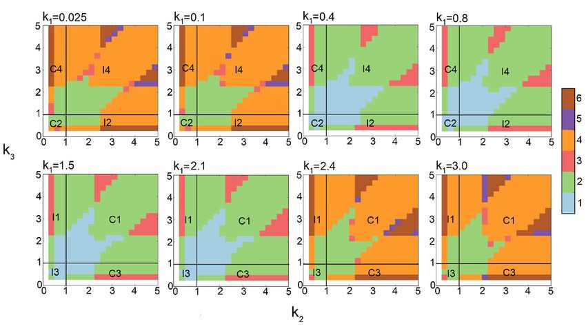
Terebus et al.                                                                                                         Stochastic Multimodality of Feed-Forward Loops

surface on lower dimensional space often no longer reflects the                        2.3.3. Persistent Diagram of Multimodality in
topology of the original space, with results and interpretations                       Probability Landscape
likely erroneous or misleading (Manuchehrfar et al., 2021).                            We keep track of the probability peaks by recording the birth
Finding peak states by examining distinct local maxima is                              and death times of their corresponding 0-homology groups
equivalent to locating hypercubes that are critical points of                          throughout the filtration. This relationship is depicted by the
Morse index of d in the d-dimension state space. While, local                          two-dimensional persistent diagram.
maxima may be identified by comparing its probability value                               For the ith probability peak, when the threshold r reaches the
with those of all of its neighbors, all peaks regardless their                         value rb (i), the probability peak appears. We call this value the
prominence will be identified. As numerical calculation may                            birth probability pb (i) = rb (i) of peak i. When the threshold r is
introduce small errors, peaks of tiny magnitude will be included.                      lowered to a value rd (i), this peak is merged to an existing peak.
It is non-trivial to decide on a proper threshold to filter them out.                  We call this value the death probability pd (i) = rd (i) of peak i.
    Persistent homology provides a powerful method that can                            The persistence of peak i is defined as:
characterize topological features of high-dimensional probability
landscapes (Edelsbrunner et al., 2002; Carlsson, 2009). Here,                                                   pers(i) ≡ pb (i) − pd (i).                        (3)
we use newly developed cubic complex algorithm to compute
homology groups1 and quantitatively assess the exact topology                          The persistent diagram plots peak i using the birth probability
of the 9-dimensional probability landscape.                                            pb (i) as the y-coordinate and the death probability pd (i) as the
                                                                                       x-coordinate. The number of dots on the persistent diagram
2.3.1. Homology Groups                                                                 corresponds to the number of probability peaks. Those that are
We use homology groups from algebraic topology to characterize                         further off the diagonals are the more prominent probability
the probability landscape. Homology group provides an                                  peaks as their persistences are larger.
unambiguous and quantitative description on how a space
is connected. It returns a set of algebraic groups describing
topological features of holes of various dimensions in the                             3. RESULTS
space. The rank of each i-th groups counts the number of                               3.1. Multimodality and Persistent
linearly independent holes in the corresponding ith dimension.
                                                                                       Homology of FFLs
For example, Rank(H0 ) counts the number of connected
                                                                                       For each FFL network, we first compute its probability landscapes
components (0th dimensional holes).
                                                                                       p = p(xA , xB , xC , xa , xb , xc , xbA , xcA , xcB ) at the steady-state under
2.3.2. Persistent Homology                                                             various conditions of model parameters. Here, xA , xB , and xC are
Persistent homology measures the importance of these                                   copy numbers of proteins A, B, and C, respectively; xa , xb , and xc
topological features (Edelsbrunner et al., 2002), and has been                         are copy numbers of genes a, b, and c, respectively; xbA and xcA
applied in studies of chemical compounds and biomolecules (Xia                         are copy numbers of genes b and c bound by protein A; xcB is the
and Wei, 2014, 2015; Xia et al., 2015). Here, we focus on                              copy number of gene c bound by protein B.
the topological features of probability peaks, including their                             Our results show that the 8 types of FFLs can exhibit up
appearance and disappearance. They are measured by persistent                          to six different phenotypes of mono- and multimodality at
homology of the 0-th homology group. Specifically, we take the                         different conditions in the parameter spaces we investigated. An
probability p(x) as a height function, and construct a sequence of                     illustration of these six different types of multimodality is shown
topological spaces using thresholds {ri } for p(x):                                    in Figure 2.
                                                                                           We further computed their 0-th homology groups at varying
                 1 = r0 > r1 > r2 > · · · > rin−1 > rin = 0,                (1)        sea level of probability. The number of peaks, the birth, and death
                                                                                       probability associated with each peak in Figure 2 are shown in
The superlevel sets {Xi } has Xi = {x ∈ X|p(x) ≥ ri },                                 the persistent diagrams of Figure 3.
which corresponds to the threshold ri . The sequence {Xi } gives
a sequence of subspaces, which is called filtration:                                   3.1.1. Behavior of FFLs From Stochastic Models
                                                                                       Differ From Deterministic ODE Models
          ∅ ≡ Xi0 ⊂ Xi1 ⊂ Xi2 ⊂ · · · ⊂ Xin−1 ⊂ Xin ≡ ,                    (2)        The behavior of FFL network modules revealed from our
                                                                                       stochastic models are fundamentally different from that of
As the threshold changes, the peak of a probability landscape
                                                                                       deterministic models of ordinary differential equations (ODEs).
emerges from the sea-level at a specific threshold, which is
                                                                                       ODE models are based on kinetics of law of mass action and
the birth time of the corresponding 0-homology group in the
                                                                                       are used to calculate the mean concentrations of A, B, and C
filtration. It disappears as an independent component when
                                                                                       at equilibrium state. However, they do not provide accurate
merged with a prior peak at a particular threshold, which is called
                                                                                       pictures on the degree of multimodality. For example, the steady-
the death time. When the sea-level recedes to the ground level at
                                                                                       state ODE solutions with respect to different gene occupancy for
p(x) = 0, only the first peak remains.
                                                                                       mass action kinetics show that there are at most six phenotypic
1 Tian,W., Manuchehrfar, F., Wagner, H., Edelsbrunner, H., and Liang, J. (2021).
                                                                                       states (see Supplementary Material for more details). However,
Persistent homology and moment of probability landscapes of stochastic reaction        as there are no probabilistic considerations, conclusions drawn
networks and their changes.                                                            from ODE models can be problematic.

Frontiers in Genetics | www.frontiersin.org                                        5                                            July 2021 | Volume 12 | Article 645640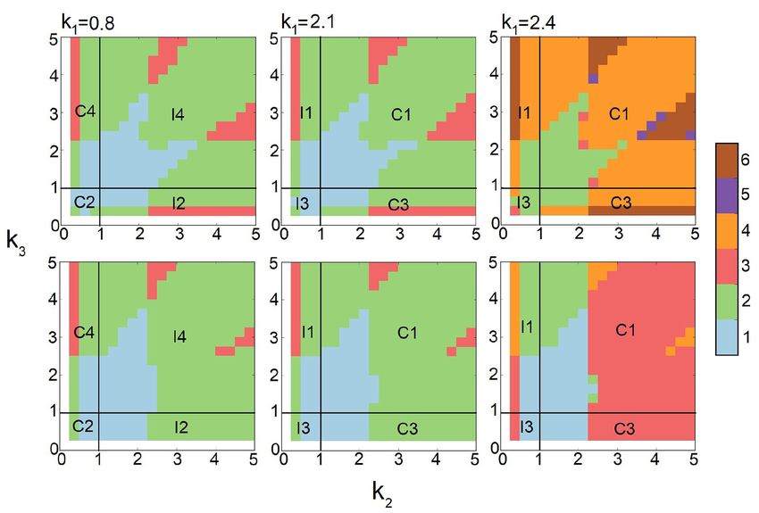
Terebus et al.                                                                                                           Stochastic Multimodality of Feed-Forward Loops

 FIGURE 2 | Examples of multimodality exhibited by feed-forward loop (FFL) network motifs. The steady-state probability landscape can exhibit up to 6 different
 multimodes. The illustrative examples are as follows: 1 peak (red), coherent FFL of type C1 when k1 = 1.2, k2 = 1.2, and k3 = 1.2; 2 peaks (yellow), either in protein B
 with coherent FFL of type C1, where k1 = 3.0, k2 = 1.2, and k3 = 1.2, or in protein C with coherent FFL of type C1, where k1 = 1.2, k2 = 6.0, and k3 = 6.0; 3 peaks
 (green), coherent FFL of type C1, where k1 = 1.2, k2 = 6.0, and k3 = 3.6; 4 peaks (light-blue), coherent FFL of type C1 exhibits two peaks for protein B and two
 peaks for protein C, where k1 = 3.0, k2 = 6.0, and k3 = 6.0; and 6 peaks (purple), coherent FFL of type C1 exhibit two peaks for B and three peaks for C, where
 k1 = 3.0, k2 = 6.0, and k3 = 3.6.

 FIGURE 3 | Persistent diagrams (PDs) of feed-forward loop (FFL) network modules of Figure 2 exhibiting different multimodalities. Red: The probability landscape
 with monomodality. Yellow: These two PDs depict the two steady-state landscapes exhibiting bimodality. Green, light blue, and purple: These three PDs depict the
 landscape exhibiting tri-modality, 4-modality, and 6-modality, respectively.

   An example of the diverging results between ODE and                                     A further example is provided by the FFL of type I1. Here,
stochastic models is shown in Figure 4A for an FFL of C1                                the ODE model predicts the existence of three phenotypes
type. The mean values of C obtained from the ODE model                                  at k1 = 2.7, k2 = 0.4, and k3 = 1.8 (Figure 4B, green
(vertical blue line) and the expectation computed from the                              vertical lines). However, the stochastic model shows that
probability landscape (vertical purple line) diverge from each                          there is only one stability peak. Although the mean value
other (Figure 4A). There are three different phenotypic states                          of C obtained from the ODE model and the expected C
by the ODE model (green lines, Figure 4A), which are different                          value computed from the probability landscape largely
from the bimodal probability distribution obtained from the SCK                         overlap, the ODE model provides no information on
model (Figure 4A).                                                                      phenotypical variability. Overall, stochastic models provide

Frontiers in Genetics | www.frontiersin.org                                         6                                              July 2021 | Volume 12 | Article 645640
Terebus et al.                                                                                                                Stochastic Multimodality of Feed-Forward Loops

 FIGURE 4 | Comparing feed-forward loop (FFL) behavior by Accurate Chemical Master Equation (ACME) and by deterministic ordinary differential equation (ODE)
 models. (A) shows the results of FFL of C1 type for (k1 , k2 , k3 ) = (2.4, 4.5, 1.8). The exact results obtained using ACME exhibit bimodality in protein C (red curve), while
 trimodality is predicted by the deterministic ODE model (green vertical lines). The mean copy number from ACME (purple vertical line) is also different from the that
 from ODE (blue vertical line). (B) shows the results of FFL of I1 type for (k1 , k2 , k3 ) = (2.4, 0.4, 1.8). The exact results obtained using ACME exhibit monomodality in
 protein C (red curve), while deterministic ODE model predicts trimodality (green vertical lines), even though the mean copy number of protein C are the same between
 ACME and ODE models (purple and blue vertical lines, respectively).

accurate and rich information that are not possible with ODE                               buffer ACME algorithm. The analysis using persistent homology
models.                                                                                    further allows us to quantitatively characterize the exact topology
                                                                                           of the landscape. Together, we are able to obtain the full phase
3.1.2. Behavior of FFLs From Exact Solution to dCME                                        diagrams on the phenotype of multimodality of FFLs at different
by ACME Can Be Differ From That by Stochastic                                              combinations of parameter values (Figure 6).
Simulation Algorithm                                                                           Altogether, we compute 10,812 probability landscapes of the
Results from simulations using SSA may differ from the exact                               8-types of FFL modules. Depending on the values of k1 , k2 , and
solution to dCME obtained using ACME. We illustrate this using                             k3 , each phase diagram shown depicts the behavior of four types
two incoherent FFLs, one at (k1 , k2 , k3 ) = (3.0, 0.5, 5.0) of I1-                       of FFLs, one for each of the four quadrants formed by the two
FFL (Figures 5A–C) and another at (k1 , k2 , k3 ) = (0.1, 2.75, 5.0)                       straight lines of k2 = 1 and k3 = 1 (Figure 6), with the type
(Figures 5D–F) of the I4-type FFL. The exact steady-state                                  of FFL labeled accordingly. The specific types also depend on
probability landscape of the I1-FFL network computed using                                 k1 , which is listed at the top of each plot (Figure 6). As a result,
ACME is multimodal, exhibiting two peaks in protein B and                                  we have gained comprehensive and accurate characterization of
two peaks in protein C (Figure 5A). However, these peaks are                               the multimodality phenotypes of this type of important network
not definitive when 30,000 reaction trajectories up to 2,500 s are                         modules.
simulated using SSA (upper plots, Figures 5B,C). Bimodality in
proteins B and C becomes only definitive when simulation time                              3.2.1. Monomodality
is extended to 5,000 s (lower plots, Figures 5B,C).                                        As shown in Figure 2, the steady-state probability landscape of
    The exact steady-state probability landscape of the I4-FFL                             the FFL at k1 = k2 = k3 = 1.2 exhibits one probability peak.
network computed using ACME exhibits tri-modality in protein                               At this condition, it is a coherent FFL of type C1. The projected
C and bimodality in protein B (Figure 5D). However, tri-                                   distributions of B and C exhibit monomodality and has only one
modality is not clearly captured when the reaction trajectories                            peak (Figure 2, red) when the values of intensities k1 , k2 , and k3
are < 2, 500 s (upper plot, Figure 5E), and becomes definitive                             are close to 1.0 (Figure 6). Overall, there is only one phenotypic
only after 5,000 s (lower plot, Figure 5E). In addition, bimodality                        state when the regulations intensities in FFL are weak.
in protein B is not captured, even when the reaction trajectories
are at 5, 000 s (upper and lower plot, Figure 5F).
                                                                                           3.2.2. Bimodality
                                                                                           The steady-state probability landscape of FFLs can exhibit two
3.2. Phase Diagrams of Multimodality in                                                    types of bimodality (colored yellow in Figure 2). The first type
FFLs                                                                                       occurs when k1 < 0.4 or k1 > 2.4, with bimodality in protein
Current studies of stochastic networks are limited to their                                B while monomodality in protein C. This is illustrated as green
behavior under a few selected conditions. Here, we explore the                             regions in Figure 6 shown at the two top-left and the two bottom
multimodality of all eight types of FFLs under broad conditions                            right phase diagrams where k1 ∈ {0.025, 0.1, 2.4, 3.0}. That is, if
of synthesis, degradation, binding, and unbinding as outlined in                           the regulation intensities of k1 and k2 are about two-fold different
Table 1. This is made possible by the efficiency of the multi-finite                       either way, bimodality in B arises.

Frontiers in Genetics | www.frontiersin.org                                            7                                                 July 2021 | Volume 12 | Article 645640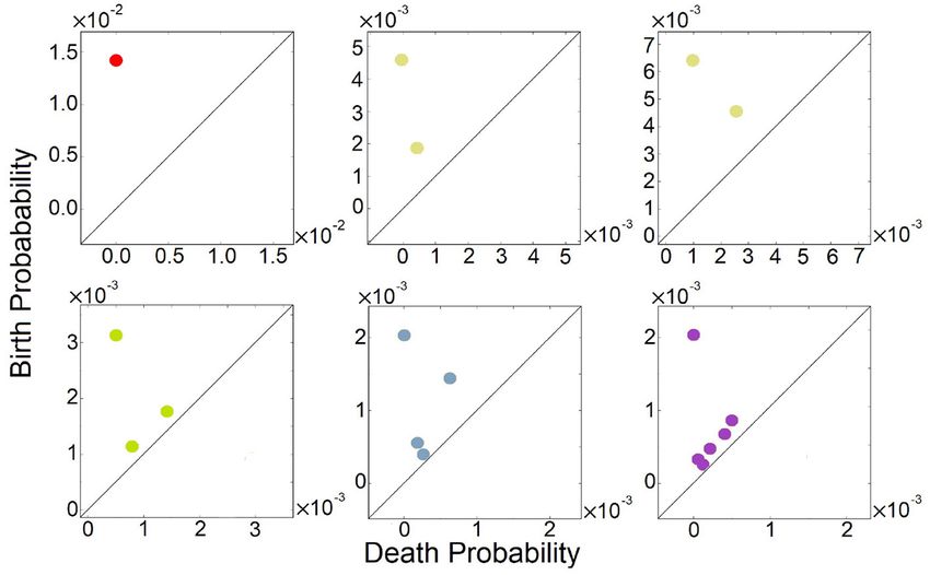
Terebus et al. Stochastic Multimodality of Feed-Forward Loops
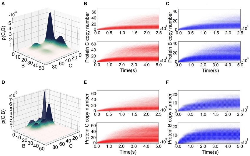
FIGURE 5 | Comparing landscapes from Accurate Chemical Master Equation (ACME) and reaction trajectories from the stochastic simulation algorithm (SSA). (A)
Probability surface projected onto the (B, C)-plane for the feed-forward loop (FFL) with (k1 , k2 , k3 ) = (3.0, 0.5, 5.0). There is bimodality in both proteins B and C. (B,C)
The reaction trajectories computed from SSA corresponding to condition in (A) for proteins C and B, respectively. The upper plots are for 2,500 s and lower plots are
for 5,000 s. SSA does not capture the bimodality of proteins B and C until 2,500 s. (D) The probability surface projected onto (B−C) plain for FFL with
(k1 , k2 , k3 ) = (0.1, 2.75, 5.0). There is tri-modality in protein C and bimodality in protein B. (E,F) Corresponding reaction trajectories in proteins C and B, respectively.
Upper plots are for the results for 2,500 s and lower plots are for 5,000 s. SSA does not capture tri-modality of protein C until 2,500 s. In addition, SSA fails to capture
bimodality in protein B.
The second type of bimodality occurs when 0.4 ≤ k1 < k1 is weak, the steady-state probability landscape exhibits
2.4, where protein C exhibit bimodality while monomodality multimodality only when the other two regulation intensities,
is maintained in B. This is illustrated as green regions in namely, k2 and k3 are strong. As shown in Figure 6, there are two
the remaining phase diagrams of Figure 6, where k1 ∈ groups of FFLs based on the characteristics of the multimodality
{0.4, 0.8, 1.5, 2.1}. they exhibit: One group consists of FFLs of C2 , C4 , I1 , and
I3 types, where tri-modality of output protein C always exists,
3.2.3. Tri-modality as long as k2 and k3 are at least about two-fold different. The
The steady-state probabilistic landscape of FFL can exhibit tri- other group consists of FFLs of C1 , C3 , I2 , and I4 types where
modality (green, Figure 2). There are three possible phenotypes the signs of the regulations that the output node C receives
in protein C while monomodality in protein B is maintained. from B and A are the same (both activation or both inhibition).
Trimodal regions are colored red in the phase diagrams of Tri-modality occurs when the regulations k2 and k3 have very
Figure 6. They arise when the difference in rates k2 and k3 is at distinct values.
least about two-fold and 0.4 ≤ k1 ≤ 2.1. Overall, protein B can exhibit either mono- or bimodality,
and protein C can exhibit mono-, bi-, or tri-modality on the
3.2.4. Multimodality probability landscape.
The steady-state probability landscape of the FFL can exhibit 4
to 6 probability peaks (orange, purple, and green, respectively,
in Figure 2). Landscapes with 4 modes have bimodality in both 3.3. Increasing Input Intensity Amplifies
protein B and protein C. Those with 5 modes has bimodality Multimodality in FFL
in B and tri-modality in C. Landscapes with 6 modes exhibit To understand how input intensity affect the response of FFL
bimodality in B and tri-modality in C. Inspection on the networks, we examine their behavior under different input
conditions indicates that when the regulations are strong; i.e., conditions. Specifically, we examine how different synthesis
when k1 , k2 , and k3 ≥ 2.1, FFLs exhibit very well-defined rate sA of protein A affects the number of modes in proteins
multimodality peaks. However, when the regulation intensity B and C.
Frontiers in Genetics | www.frontiersin.org 8 July 2021 | Volume 12 | Article 645640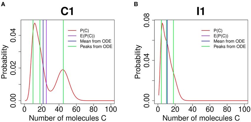
Terebus et al.                                                                                                              Stochastic Multimodality of Feed-Forward Loops

 FIGURE 6 | Phase diagrams of multimodality of Feed-forward loop (FFL) network modules based on 10,812 steady-state probability landscapes at different condition
 of regulation intensities for all 8 types of FFL network modules. Monomodality occurs when 0.4 ≤ k1 ≤ 2.1 and k2 , k3 intensities are moderate, i.e., 0.4 ≤ k1 ≤ 3
 (blue region when k1 = 0.4, 0.8, 1.5, and 2.1). Bimodality may occur for different combinations of regulation intensities. When k1 intensity is either very high (2.4 ≤ k1 )
 or very low (k1 ≤ 0.1), bimodality occurs when k2 , k3 intensities are moderate, i.e., 0.4 ≤ k1 ≤ 3. When k1 intensity is moderate (0.4 ≤ k1 ≤ 2.1), bimodality occurs
 when at least one of the other regulation intensities k2 or k3 is high. Tri-modality occurs when k1 is moderate (0.4 ≤ k1 ≤ 2.1) and either k2 or k3 is moderate.
 Multimodality occurs when k1 is low or high (k1 ≤ 0.4 or k1 ≥ 2.1), and at least either k2 or k3 is high. Color scheme (vertical bar): Blue, green, red, orange, purple,
 and brow represent regions with one, two three, four, five, and six peaks, respectively.

   We first carry out computations and broadly survey the                                 3.4. Binding and Unbinding Dynamics Are
behavior of FFLs at strong input intensity, where sA is set to 10.0.                      Critical for Multiple Phenotypic Behavior
The values of k2 and k3 are sampled broadly, and k1 is tested for                         Results obtained so far are based on the assumption of slow
three different values of k1 = 0.8, 2.1, and 2.4. The results are                         binding (rbA = rcA = rcB = 0.005) and unbinding (fbA =
summarized in Figure 7 (top row). We then similarly survey the                            fcA = fcB = 0.1) reactions, which we call the generic case. When
behavior of FFLs at decreased synthesis intensity of protein A,                           the FFL network slowly switches between phenotypic states, the
with sA = 3.0 (Figure 7, bottom row).                                                     process of synthesis degradation of protein C has sufficient time
   There are clear changes in the mode of multimodality of FFLs.                          to converge to equilibrium at each phenotypic state of gene c. An
At k1 = 0.8 and k1 = 2.1 (Figure 7, left and center columns),                             important questions is how slow the promoter dynamics need
when protein A synthesis rate sA is reduced from 10.0 (top) to                            to be for FFLs to exhibit multiple phenotypes, without feedback
3.0 (bottom), regions with one (blue) and three (red) peaks are                           loops or cooperatively.
reduced. In addition, certain areas of the tri-stable (red) regions                           To answer this question, we explore the behavior of FFLs
become bimodal (green).                                                                   under different binding and unbinding dynamics of gene c for
   At larger k1 = 2.4 (Figure 7, right column), the FFLs                                  an FFL of type I1. In this case, protein A activates protein B and
exhibits dramatic changes in the modes of multimodality when                              protein C, while protein B inhibits protein C (see Figure 1B).
synthesis rate sA of protein A is reduced from 10.0 (top) to 3.0                          With slow binding kinetics as described above, the output C of
(bottom). In many regions, one or more stability peaks disappear.                         this FFL exhibits three stability peaks. These are at the expression
There are regions with two peaks at sA = 10.0 that become                                 level of protein C of (1) C = 0, corresponding to the condition
monomodal. There are also regions of six peaks that become                                when gene c is inhibited by B, (2) C = 9, corresponding to the
those of four peaks. This is due to the loss of one stability                             basal level of C expression, and (3) C = 49, when C expression is
peak from three in protein C. In addition, large regions with                             activated by A. We then fix the regulation intensities at k1 = 3.0,
four peaks (orange) disappear and become either regions with                              k2 = 0.025, and k3 = 5.1, and examine how the number
two peaks (green) or with three peaks (red). Overall, we can                              of phenotypic states is affected by gene c binding dynamics
conclude that high-input intensity represented by high sA rate                            (Figure 8).
for protein A induces changed phenotypes of multimodality                                     We first set the binding affinities between gene c and
in FFLs.                                                                                  protein A and between gene c and protein B to the same

Frontiers in Genetics | www.frontiersin.org                                           9                                               July 2021 | Volume 12 | Article 645640
Terebus et al.                                                                                                             Stochastic Multimodality of Feed-Forward Loops

 FIGURE 7 | Effects of input intensity on multimodality of Feed-forward loops (FFLs). The phase diagrams of the number of stability peaks in the steady-state
 probability landscapes at strong input intensity sA = 10.0 (top row) and weak input intensity sA = 3.0 (bottom row) for different k2 and k3 at three different conditions
 of k1 = 0.8, 2.1, and 2.4. Color scheme (vertical bar): Blue, green, red, orange, purple, and brown represent regions with one, two, three, four, five, and six peaks,
 respectively.

values, and change them together to n-fold of the generic case,                          3.5. Gene Duplication Can Enrich
where n ∈ {0.5, 2, 8, 16}. For slower binding and unbinding                              Phenotypic Diversity and Enlarge Stable
dynamics (yellow line for n = 0.5, Figure 8A), the modes
                                                                                         Regions of Specific Multimodality of FFLs
of the distribution of the output of protein C are even better
                                                                                         Gene duplication provides a basic route of evolution (Lynch
distinguished. However, when both binding and unbinding rates
                                                                                         and Conery, 2000) and is an important driver of phenotypical
are increased to n = 8 fold (green line), the probability peak at                        diversity in organisms (Conrad and Antonarakis, 2007). Here, we
C = 9, which corresponds to basal level of C expression, merges                          study how gene duplication affects the phenotypes of FFLs.
with the probability peak at C = 0. At n = 16, the distribution of                           We examine how duplication of gene c and separately
C is bimodal.                                                                            duplication of gene b affect the behavior of the FFL network
    We then keep the biding affinity between gene c and protein                          modules. With two copies of gene c, there can be six possible
A unchanged and alter only the binding affinity between gene                             states of gene c activation. Depending on whether the promoter
c and protein B by n-fold, where n ∈ {0.5, 2, 8, 16}. When                               sites of both copies of gene c are free or occupied by either protein
the binding affinity increases (e.g., n = 8), the probability                            A or protein B, we have for both c genes to have unoccupied,
peak at C = 9 disappears, while the probability peak at high                             protein A bound, or protein B bound promoter site. This can be
copy number of C = 49 robustly remains, although with less                               denoted as a triplet (c, cA, cB), which can take any of the possible
magnitude (Figure 8B).                                                                   values of (2, 0, 0), (0, 2, 0), (0, 0, 2), (1, 1, 0), (1, 0, 1), and (0, 1, 1).
    When only the biding affinity between gene c and protein                             For the case when there are two copy number of gene B, there are
A is altered while that between gene c and protein B is held                             three possible states of gene b activation, depending on whether
constant (Figure 8C), the probability peak at the basal level of                         the promoter site of both copies of gene b are free or occupied by
C expression (C = 9) diminishes when the binding affinity                                protein A. This can be denoted as a duplicate (b, bA), which can
increases (e.g., n = 8). However, the probability peak at C = 49                         take any of the possible values of (2, 0), (1, 1), or (0, 2).
becomes more prominent. At n = 8, the distribution of C is                                   The phase diagrams of the number of modes of stability peaks
tri-modal. At n = 16, it becomes bimodal. This indicates that                            are shown in Figure 9, when there is only one copy of both gene
multiple phenotypes arise in FFLs when the unbinding rate is                             b and gene c (first row), when there are two copies of gene c
about an order of magnitude smaller than the expression rate of                          but one copy of gene b (second row), and when there are two
the protein.                                                                             copy number of gene b but one copy of gene c (third row). The

Frontiers in Genetics | www.frontiersin.org                                         10                                               July 2021 | Volume 12 | Article 645640
Terebus et al. Stochastic Multimodality of Feed-Forward Loops
FIGURE 8 | Effect of binding dynamics on the modality of protein C in the feed-forward loop (FFL) network of type I1, with (k1 , k2 , k3 ) = (3.0, 0.025, 5.1). (A) Effects
when binding affinity between gene c and both protein A and protein B are altered by n-fold, where n ∈ {0.5, 2, 8, 16}. At slower binding (yellow line), the modes of
distribution of protein C are well-distinguished. However, when the binding and unbinding rates increased to 8 (green line), the peak at C = 9 disappears. At n = 16,
bimodality is observed in protein C. (B) Effects when only the binding affinity of gene c and protein B is altered by n-fold, where n ∈ {0.5, 2, 8, 16}. When the binding
affinity of gen c and protein B increases, the peak at C = 9 disappears, while the peaks at C = 49 robustly remains. However, the peak at C = 49 becomes less
significant. (C) Effects when only the binding affinity of gen c and protein A is altered by n-fold, where n ∈ {0.5, 2, 8, 16}. At high binding affinity, the peak at C = 9
disappears while the peak at C = 49 becomes more prominent.
conditions are k1 = 0.025, 0.8, 1.5, and 2.4, for different values of switching. This is reflected in reduced monomodal regions,
k2 ∈ [0.1, 5] and k3 ∈ [0.1, 5], where there are slow binding and and enlarged multimodal regions where there are 4 (orange), 5
unbinding (rbA = rcA = rcB = 0.005, fbA = fcA = fcB = 0.1). Each (purple), and 6 (brown) phenotypic states of the output C (second
phase diagram in Figure 9 consists of 400 steady-state probability and third row in Figure 9).
landscapes with a total 12 × 400 = 4, 800 landscapes. This broad Assuming that initially both copies of the gene were
range of parameters allow us to study all 8 different modules of functioning, but subsequently one gene copy lost its biochemical
FFL network and the effects of gene c and gene b duplications. function due to mutations, we can expect two opposite types of
We examine the behavior of FFL in three different regimes scenarios to occur: If regulation intensities are strong (k2 and
of k1 : (1) When k1 ≪ 1.0 (Figure 9, first column), the bimodal k3 are large), one of the phenotypic states becomes lost (e.g.,
regions (green) expands when there are two copies of gene c green region becomes light blue, and orange region becomes
(second row), but there are no significant changes when there are red, Figure 9). If regulation intensities are weak, the duplication
two copies of gene b (third row). The overall size of multimodal of gene c or gene b can lead to enlargement of the region of
regions increases in both cases. (2) When k1 ≈ 1.0 (Figure 9, monomodality. It can also lead to the appearance of new regimes
second and third columns), the duplication of gene c (second where there are a larger number of multimodality modes (orange,
row) expands the regions with three stability peaks and reduces purple, and green regions in Figure 9). That is, gene duplication
regions with two peaks. In contrast, the duplication of gene b can create new stable states, leading to an enlarged number
(third row) has no significant effects on multimodality. (3) When of high probability states. This, however, occurs only in FFL
k1 = 2.4 (fourth column), duplication of gene c (second row) modules with strong regulations intensities. FFL modules with
expands regions with two and six stability peaks. Duplication low regulation intensities instead lose phenotypical diversity and
of gene b (third row) reduces the region with four peaks and become more robust in monomodality with enlarged region in
expands the region with five peaks. the parameter space.
These results show that introducing additional copy of gene
b or gene c not only can enrich different phenotypic behavior
but can also increase the stability of specific phenotypic states, 4. DISCUSSION
namely, enlarge regions of particular phenotypes by uniting
previously different phenotypic regions together. Overall, gene Gene regulatory networks (GRNs) play critical roles in defining
duplication can increase phenotypic diversity, and enlarge cellular phenotypes but it is challenging to characterize the
stability regions of specific multimodal states. behavior of GRNs. Although GRNs may consist of dozens
Bacterial cells have fast binding and unbinding dynamics (Ali or more of genes and proteins, their functions often can be
Al-Radhawi et al., 2019), and it is unlikely that the occurrence defined by smaller sub-networks called network motifs. How
of multiple copies of the same gene in FFLs plays significant small network motifs are responsible for complex properties such
roles in stochastic multimodality. In contrast, mammalian cells as the maintenance of multi-phenotypic behavior or modules
have slower promoter dynamics (Forger and Peskin, 2003). is poorly understood. Current widely practiced approach is
Gene duplication in FFLs may provide a natural mechanism studying network motifs using deterministic models. However,
for enriched multimodality with enhanced stochastic phenotypic this approach imposes restrictions on the types of network motifs
Frontiers in Genetics | www.frontiersin.org 11 July 2021 | Volume 12 | Article 645640Terebus et al. Stochastic Multimodality of Feed-Forward Loops FIGURE 9 | Phase diagram of the effects of gene duplication on multimodality of feed-forward loops (FFLs). First row: Phase diagrams of the modality of stability peaks when there are one copy of gene c and one copy of gene b. Second row: Phase diagrams when there are one copy of gene b and two copies of gene c. Third row: Phase diagram, when there are two copy of gene b and one copy of gene c. The first, second, and third columns are for k1 = 0.025, 1.5, and 2.4, respectively. Color scheme (vertical bar): Blue, green, red, orange, purple, and brown represent regions with one, two, three, four, five, and six peaks, respectively. capable of exhibiting multimodal phenotype to mostly feedback by Michaelis–Menten kinetics, with the additional assumption networks. that the substrate is in instantaneous chemical equilibrium with In this study, we examined the FFL network motifs, one of the enzyme–substrate complex. When ODE models are applied the most ubiquitous three-node network motifs. Although their to the reaction of one receptor and n identical simultaneously deterministic behavior is well-studied, with great understanding binding ligands, we arrive at the Hill equation, with the of their functions such as signal processing and adaptations coefficient n phenomenologically characterizing cooperativity. gained, their stochastic behavior remains poorly characterized. These kinetic models based on ODE approximations, however, Here, we showed the direct regulation path from the input are not applicable to the current study, as we are examining node to the output node and the indirect path through the strong stochasticity arising at low copy number of molecules, intermediate buffer node provide the necessary architecture where ODE models are not valid. for distinct multiple modalities. Phase diagrams of FFL in FFLs play important roles in gene regulatory networks. For Figure 6 show that FFLs of various types can exhibit different example, it is shown that several I1-FFL sub-networks control the multimodality. At large copy numbers and large volume, our process of Bacillus subtilis sporulation (Eichenberger et al., 2004; model of stochastic reaction kinetics are the same as those Mangan et al., 2006). In addition, C1-FFL network is found to based on mass action kinetics (Kurtz, 1971, 1972; Vellela be present in the L-arabinose (ara) utilization system of E. coli, and Qian, 2007), where ordinary differential equation (ODE) where araBAD is the target (gene c) activated by the intermediate models are appropriate. When ODE models are applied to gene araC and the input gene CRP. Gene araC is also activated by enzyme–substrate reactions, they can be further approximated CRP. Therefore, they form a 3-node C1 type FFL (Mangan et al., Frontiers in Genetics | www.frontiersin.org 12 July 2021 | Volume 12 | Article 645640
Terebus et al.                                                                                           Stochastic Multimodality of Feed-Forward Loops

2003). Results in this work can help to gain understanding of the            enrich phenotypic diversity. The presence and functional roles
behavior of these different types of FFLs found in gene regulatory           of gene duplication are well-known (Hurles, 2004). For example,
networks.                                                                    in human-induced pluripotent stem cells (HiPSCs), chromosome
    In addition, we have shown that input intensity affects the              12 duplication leads to significant enrichment of cell cycle related
multimodal behavior of various types of FFLs. Examples shown                 genes (Mayshar et al., 2010), in which FFL sub-networks play
in Figure 7 demonstrate that at high k1 values, input intensity              important roles. This abnormality results in increase in the
dramatically changes the multimodality as shown in the phase                 tumorigenicity of HiPSCs. Our findings may also shed light
diagrams. Our results are consistent with previous findings that             on how gene duplication affects cellular adaptation to changing
input intensity is an important factor in determining output                 environment (Kondrashov, 2012): As the support regions of
intensity of FFLs (Mangan et al., 2003; Goentoro et al., 2009; Lin           monomodality are enlarged, smaller fluctuations in regulation
et al., 2018). Here, we further demonstrated that input intensity            intensities will not switch cells with duplicated genes to a different
is also important in determining the modality of the steady-state            phenotypic state. Thus, gene duplication may help to stabilize
behavior of FFLs.                                                            the behavior of the network, so cells are better adapted to a
    In mammalian cells, slow dynamics of transcription factor                changing environment.
binding to promoter is often observed (Dermitzakis and Clark,                    Analysis of stochastic behavior of FFLs reported here have
2002; Hager et al., 2009; Lickwar et al., 2012; Tuǧrul et al., 2015;        implications in a variety of biological problems. For example,
Hasegawa and Struhl, 2019). This is likely due to the complex                the stem cell regulation network consisting of pluripotency
process of chromatin regions opening up so they become                       transcription factors Oct4 and Nanog maintain pluripotency
accessible and the slow nature of events such as promoter,                   against differentiation (Boyer et al., 2005; Chickarmane et al.,
enhancer, and mediator binding. These physical processes result              2006; Papatsenko et al., 2015; Lin et al., 2018). A component of
in highly stochastic behavior of networks. Stochastic models                 this network can be abstracted as an FFL: Nanog participates as
have demonstrated that complex multimodality phenotypes can                  the intermediate node (gene b, which is activated by Oct4 (gene
naturally arise from stochastic fluctuations when genes have                 a), and both regulate the expression of genes associated with the
distinct expression levels, a phenomenon widely observed in                  onset of differentiation or pluripotency (gene cs). In addition,
mammalian cells (Cao et al., 2018). We showed that binding and               regulation networks in hematopoietic stem cells are formed by
unbinding dynamics are critical for multi-phenotypic behavior.               two FFL networks involving β globin, GATA-1, EKLF, and FOG-
For an I1-FFL with (k1 , k2 , k3 ) = (3.0, 0.025, 5.1), Figure 8             1. In each network, FOG-1 and EKLF function as the intermediate
highlighted that binding and unbinding rates affect multiple                 genes (gene b) and are activated by GATA-1 (gene a), while all of
peaks in protein C.                                                          them activate β globin (gene c) (Swiers et al., 2006). Moreover,
    Results of this study indeed showed that once stochastic                 in other stem cell differentiation networks, there are several sub-
fluctuations between distinct expression levels due to slow                  networks that exhibit behaviors of different types of FFLs. For
promoter dynamics are considered, FFLs can exhibit complex                   example, Klf4 (gene a) activates Pou5f1 (gene b) and inhibits Sox2
multimodal phenotypes. When the expression levels of the                     (gene c), while Pou5f1 activated Sox2 (Onichtchouk et al., 2010;
output gene (gene c) at the inhibited, basal, and activated states           Okawa et al., 2016), as in the C3-type FFL (Figure 1).
are well-separated, three distinct phenotypes arise. Combined                    In summary, we have constructed and analyzed the exact high-
with two additional possible phenotypes of different levels of               dimensional steady-state probability landscapes of FFLs under
gene b expression, we can have up to six modalities for FFLs.                broad conditions and have constructed their phase diagrams
Furthermore, high intensity of input amplifies multimodality                 in multimodality. These results are based on 10,812 exactly
in FFLs, suggesting that the FFL architecture are favored for                computed probability landscapes and their topological features
maintaining multiple phenotypic states. In addition, we find                 as measured by persistent homology. With slow binding and
that regulation intensities are key determinants of specific                 unbinding dynamics of transcription factor binding to promoter,
stochastic behavior of FFLs, which could be tuned in order                   FFLs exhibit strong stochastic behavior that is very different
to obtain any desired phenotypic behavior between 1 and 6                    from deterministic models, and can exhibit from 1 up to 6
stability modes.                                                             stability peaks. In addition, input intensity play major roles in
    Our study also revealed the roles of gene duplication.                   the phenotypes of FFLs: At weak input intensity, FFLs exhibit
When there are two copies of gene c, while one in principle                  monomodality, but strong input intensity may result in up to 6
could expect 2 × 6 = 12 different phenotypes for the                         stable phenotypes. Furthermore, we found that gene duplication
output protein C. This is, however, not observed, as the                     can enrich the diversity of FFL network phenotypes and enlarge
regulation intensities or reaction rates are not well-separated.             stable regions of specific multimodalities.
In contrast, instead of further increase in multimodality beyond                 Results reported here can be useful for constructing synthetic
six, we observe the expansion of the area of monomodality,                   networks, and for selecting model parameters, so a particular
resulting from the connectedness of regions of expression                    desirable phenotypic behavior can materialize (Jones et al., 2020).
with different rates that are merged together. Our results                   Our results can also be used for analysis of behavior of FFLs
showed that duplication of gene b and gene c not only can                    in biological processes such as stem cell differentiation and for
enrich different phenotypic behavior but can also increase the               design of synthetic networks with desired phenotype behavior.
stability of certain phenotypic states, while decreasing others              We hope results reported here for different types of FFL can be
(Figure 9). We showed that in general, gene duplication can                  tested experimentally.

Frontiers in Genetics | www.frontiersin.org                             13                                        July 2021 | Volume 12 | Article 645640
You can also read


