Experimental investigation of the stable water isotope distribution in an Alpine lake environment (L-WAIVE) - Recent
←
→
Page content transcription
If your browser does not render page correctly, please read the page content below
Atmos. Chem. Phys., 21, 10911–10937, 2021
https://doi.org/10.5194/acp-21-10911-2021
© Author(s) 2021. This work is distributed under
the Creative Commons Attribution 4.0 License.

Experimental investigation of the stable water isotope distribution in
an Alpine lake environment (L-WAIVE)
Patrick Chazette1 , Cyrille Flamant2 , Harald Sodemann3 , Julien Totems1 , Anne Monod4 , Elsa Dieudonné5 ,
Alexandre Baron1 , Andrew Seidl3 , Hans Christian Steen-Larsen3 , Pascal Doira1 , Amandine Durand4 , and
Sylvain Ravier4
1 Université Paris-Saclay, Laboratoire des Sciences du Climat et de l’Environnement (LSCE), CEA-CNRS-UVSQ,
UMR CNRS 8212, CEA Saclay, 91191 Gif-sur-Yvette, France
2 LATMOS/IPSL, Sorbonne Université, UVSQ, CNRS UMR 8190, Paris, France
3 Bergen and Bjerknes Centre for Climate Research, University of Bergen, Bergen, Norway
4 Aix Marseille Univ, CNRS, LCE, Marseille, France
5 Université du Littoral Côte d’Opale, Laboratoire de Physico-Chimie de l’Atmosphère (ULCO/LPCA),

59140 Dunkirk, France

Correspondence: Patrick Chazette (patrick.chazette@lsce.ipsl.fr)

Received: 18 November 2020 – Discussion started: 1 December 2020
Revised: 8 May 2021 – Accepted: 11 June 2021 – Published: 20 July 2021

Abstract. In order to gain understanding on the vertical         In parallel, throughout the campaign, liquid water samples
structure of atmospheric water vapour above mountain lakes       of rain, at the air–lake water interface, and at 2 m depth in
and to assess its link with the isotopic composition of          the lake were taken. A significant variability of the isotopic
the lake water and with small-scale dynamics (i.e. valley        composition was observed along time, depending on weather
winds, thermal convection above complex terrain), the L-         conditions, linked to the transition from the valley boundary
WAIVE (Lacustrine-Water vApor Isotope inVentory Experi-          layer towards the free troposphere, the valley wind intensity,
ment) field campaign was conducted in the Annecy valley in       and the vertical thermal stability. Thus, significant gradients
the French Alps during 10 d in June 2019. This field cam-        of isotopic content have been revealed at the transition to the
paign was based on an original experimental synergy be-          free troposphere, at altitudes between 2.5 and 3.5 km. The
tween a suite of ground-based, boat-borne, and two ultra-        influence of the lake on the atmosphere isotopic composition
light aircraft (ULA) measuring platforms implemented to          is difficult to isolate from other contributions, especially in
characterize the thermodynamic and isotopic composition          the presence of thermal instabilities and valley winds. Nev-
above and in the lake. A cavity ring-down spectrometer and       ertheless, such an effect appears to be detectable in a layer
an in-cloud liquid water collector were deployed aboard one      of about 300 m thickness above the lake in light wind condi-
of the ULA to characterize the vertical distribution of the      tions. We also noted similar isotopic compositions in cloud
main stable water isotopes (H16       18          2 16
                                2 O, H2 O and H H O) both        drops and rainwater.
in the air and in shallow cumulus clouds. The temporal evo-
lution of the meteorological structures of the low troposphere
was derived from an airborne Rayleigh–Mie lidar (embarked
on a second ULA), a ground-based Raman lidar, and a wind         1   Introduction
lidar. ULA flight patterns were repeated several times per
day to capture the diurnal evolution as well as the variabil-    Why are the vertical structures of the stable isotope of the
ity associated with the different weather events encountered     water vapour field in the lower troposphere only sparsely
during the field campaign, which influenced the humidity         documented above Alpine lakes? This is in part due to the
field, cloud conditions, and slope wind regimes in the valley.   complexity and fast-evolving nature of the low-level atmo-
                                                                 spheric circulation in Alpine-type valleys which is intimately

Published by Copernicus Publications on behalf of the European Geosciences Union.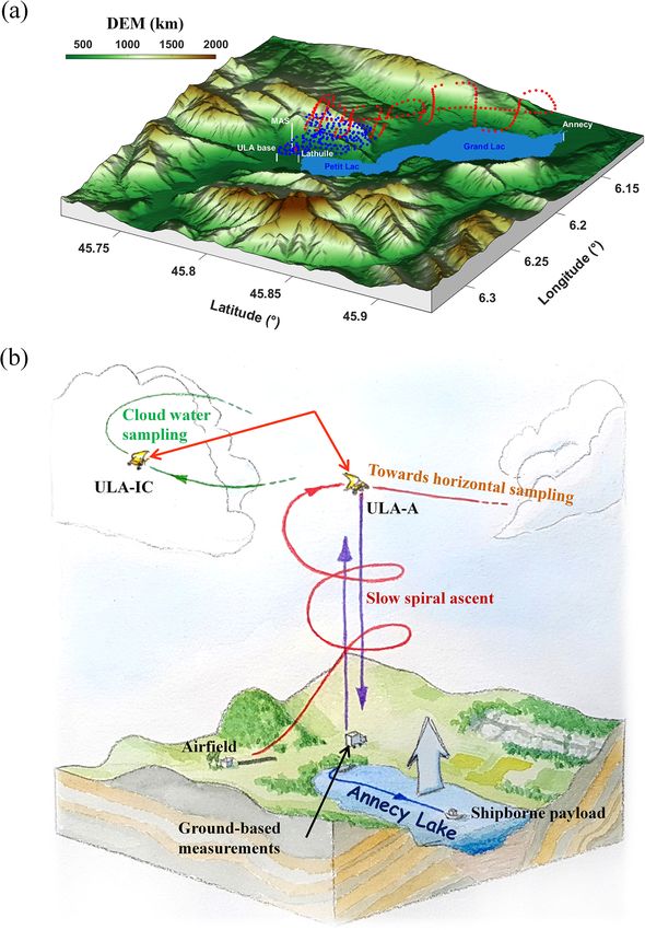
10912                                                    P. Chazette et al.: Water isotope profiles in Alpine lake (L-WAIVE)

linked to the surrounding orography interacting with the           ing the second largest natural glacial lake in France, Lake
synoptic-scale circulation. Thermally driven wind systems          Annecy is expected to play a substantial role for the regional
may be induced by hilly terrain, such as slope, mountain, and      hydrometeorology.
plateau winds (Kottmeier et al., 2008). Such winds result in          The overarching scientific objective of L-WAIVE field
mountain-venting phenomena that control the variability of         campaign is to study the vertical distribution of the water
the water vapour field in mountain catchment on very small         vapour contents and its heterogeneity over Lake Annecy.
timescales. Furthermore, small-scale inhomogeneity in soil         For this purpose, we have implemented an original multi-
properties across a mountain valley, as well as lake breezes       platform experimental approach based on continuous high-
resulting from land–lake temperature contrasts, may also in-       resolution vertical profiling of tropospheric water vapour,
duce the development of thermal circulations, particularly on      temperature, and wind, as well as scattering layers (aerosols,
clear-sky days, modifying the wind, humidity, and tempera-         clouds) in the valley. Continuous atmospheric sampling was
ture fields on small spatial scales. The interaction of slope-     carried out by lidars together with airborne and boat-borne
driven and secondary circulations can furthermore influence        measurements of stable water isotopes (H16             2
                                                                                                                  2 O, H HO and
the thermodynamical environment in the valley by the forma-          18
                                                                   H2 O) in vapour, as well as liquid water sampling in the lake,
tion of convergence lines. Such convergence lines may favour       clouds, and precipitation. A consolidated vision of water iso-
the formation of shallow clouds and in some cases even             topes across the air–water compartments in the lake area is
deep convection (Barthlott et al., 2006). Interaction with the     proposed. Special emphases are made on the interface be-
synoptic-scale circulation can lead to the formation of strong,    tween the lake and the atmosphere, as well as at the boundary
gusty down-valley winds such as foehn events (Drobinski et         with the free troposphere.
al., 2007) and gap flows (Flamant et al., 2002; Mayr et al.,          It is worth noting that we have defined such an obser-
2007) that can also contribute to rapid modifications of the       vational strategy including ultra-light aircraft (ULA) means
water vapour field in mountain catchment areas.                    because measurements tall towers only provide incomplete
   Stable water isotopes have long been used as a tool to          information on the link between the different compartments
study processes in lacustrine and hydrologic systems (see          in the free troposphere where the processes of mixing and
review by Gat, 2010), as well as evapotranspiration (e.g.          distillation occur (e.g. Griffis et al., 2016; Steen-Larsen et
Berkelhammer et al., 2016). For instance, an early study           al., 2013). In the past, He and Smith (1999) combined air-
based on water stable isotope measurements conducted in            borne measurements and surface sampling of the water iso-
the US Great Lakes region suggested that in the summer             tope composition to study the evaporation process over the
up to 15 % of the atmospheric water content in the atmo-           forests of New England, before the advent of high-resolution
sphere downwind of the lakes is derived from lake evapora-         laser-based spectrometers. More recent available airborne
tion (Gat et al., 1994). Isotopic measurements of lake wa-         measurements of the isotope composition in the boundary
ter have shown the relative roles of evaporation from the          layer either focused on areas above the sea (Sodemann et al.,
lake surface and transpiration from surrounding vegetation         2017) or did not include measurements of the surface isotope
(Jasechko et al., 2013). The link between hydrology and            composition (Salmon et al., 2019). The use of ULA makes it
evaporation has mainly been investigated using vapour and          possible to sample the atmosphere very close to the surface
liquid water isotopes measurements gathered just above the         up to altitudes of more than 4000 m and to fly in deep valleys
Earth’s surface and samples from lake water and precipita-         (Chazette et al., 2005).
tion (e.g. Cui et al., 2016).                                         The rest of the article is divided into six sections. The ex-
   Unexploited potential remains in using stable water iso-        perimental strategy is discussed in Sect. 2, whereas the in-
topes to increase our understanding of the influence of evap-      strumental platforms operations and environmental variables
oration, boundary-layer processes, and the free troposphere        monitoring are presented in Sect. 3. In Sect. 4, we give the
for local and regional climate conditions in Alpine lakes. For     synoptic conditions of atmospheric circulation that help to
example, the depth of the atmospheric layer over which the         understand the temporal evolution of the measurements in
influence of evaporation from the lake surface is detectable,      the valley, and more generally the meteorological conditions
and how different factors control the depth of this layer are      encountered during the field campaign. Atmospheric water
still largely unknown. Detailed and comprehensive analysis         vapour and liquid water isotopes, as well as lake water iso-
of small-scale factors, such as winds in a valley, and how         tope observations made across the valley, are described in
they are related to local and larger-scale dynamics, such as       Sect. 5. In Sect. 6, the vertical distribution of water isotopes
synoptic-scale subsidence in complex terrain, are therefore        is discussed taking into account the vertical structures of
needed.                                                            the lower troposphere and the lake–atmosphere interface. We
   In order to get insights into such aspects, the L-              conclude in Sect. 7.
WAIVE (Lacustrine-Water vApor Isotope inVentory Exper-
iment) field campaign was conducted in the Annecy val-
ley (45◦ 470 N, 6◦ 120 E; in Haute-Savoie in the French Alps)
around the Lake Annecy between 12 and 23 June 2019. Be-

Atmos. Chem. Phys., 21, 10911–10937, 2021                                          https://doi.org/10.5194/acp-21-10911-2021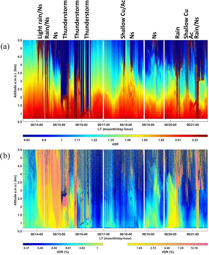
P. Chazette et al.: Water isotope profiles in Alpine lake (L-WAIVE) 10913
2 L-WAIVE experimental strategy aerosols, and winds were acquired continuously from
two co-located ground-based lidars.
To achieve the scientific and methodological objectives of the
L-WAIVE project, the field campaign was implemented in iii. For the boat-borne platform, an instrumented boat al-
the southern part of Lake Annecy (the so-called “Petit Lac”), lowed sampling the lake water by vials at the surface
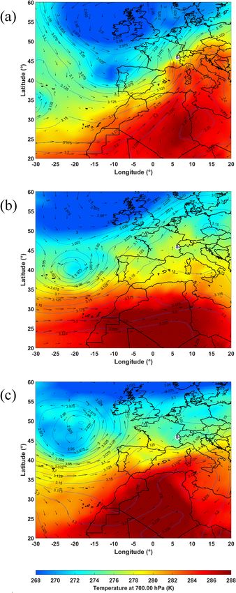
in the vicinity of the city of Lathuile (Fig. 1). Lake Annecy film and underneath (∼ 2 m deep) for the assessment of
is bordered by the city of Annecy to the north, the Massif des H2 HO and H18 2 O. A CRDS water vapour isotope anal-
Bauges to the west (2217 m above mean sea level – a.m.s.l.), yser performed measurements during 1 d at the end of
the Massif des Bornes to the East (2438 m a.m.s.l.), and the the experiment just above the lake surface in parallel
depression de Faverges to the south (where Lathuile is lo- with the lake water sampling.
cated). Lathuile is located east of the foothill of the Roc des
These different platforms are presented in Fig. 1 together
Boeufs (1774 m a.m.s.l.) to the west of the “Petit Lac” and
with a view of the experiment site.
the Tournette summit (2350 m a.m.s.l.) to the east. Lake An-
necy, at a mean altitude of 446.7 m a.m.s.l., covers an area 2.2 Deployment
of roughly 27.5 km2 and has a mean (maximum) depth of
41.5 m (82 m). Depending on the weather conditions, airborne platforms
were deployed several times a day to document the temporal
2.1 Measurement platforms evolution of the atmospheric boundary layer over the lake.
The days of operation of all platforms are summarized in Ta-
Two airborne, one boat-borne, and one ground-based instru-
ble A1 of Appendix A. The ground-based water vapour, tem-
mented platforms were deployed in the vicinity of Lathuile
perature, and aerosol lidar operated continuously between 12
in order to monitor humidity, temperature, wind, clouds, and
and 21 June in the morning (gathering over 220 h of data),
aerosols in the lower troposphere over Lake Annecy and the
while the ground-based wind lidar (WL) operated continu-
surrounding valley environment, as well as to conduct mea-
ously between 14 and 23 June in the morning (acquiring also
surements at the interface between the atmosphere and the
over 220 h of data). A total of 22 successful flights were con-
lake, and in the lake. A brief overview of the platforms is
ducted with ULA-A between 13 and 19 June, while ULA-IC
given below, whereas the details on the instrumental pay-
performed 15 flights between 14 and 20 June. Valid cloud
loads are given in Sect. 3:
water samples were only obtained during the last three ULA-
i. Airborne platforms included the following: IC flights.
The CRDS previously installed on ULA-IC was mounted
a. One ultra-light aircraft (ULA) was mainly dedi- on the boat from 21 to 22 June. Boat-borne CRDS observa-
cated to remote sensing measurements. It allowed tions were made at the surface of the lake on the last outings
exploring the two- or three-dimensional structure of the boat. Nevertheless, lake water samples were taken on
of the lower troposphere thanks to a polarized 14 occasions during the field campaign (see Appendix A).
Rayleigh–Mie lidar. It also carried a Global Po- Finally, 28 samples of precipitation were taken during the
sitioning System (GPS) device and a meteorolog- campaign (7 of which were taken on 15 June in the after-
ical probe (pressure, temperature, relative humid- noon) between 11 and 22 June 2019.
ity). This will be referred to as “aerosol ULA” On days when both ULA flew in coordinated patterns (13,
(ULA-A) in the following. 16–20 June), flights typically began with a profiling sequence
b. A second ULA carried both a cavity ring-down between the surface and ∼ 4 km a.m.s.l., which was carried
spectrometer (CRDS) water vapour isotope anal- out in the vicinity of the two ground-based vertically point-
yser, a meteorological probe for pressure, air tem- ing lidars (see Fig. 2). Soundings with levelled legs (see dot-
perature, GPS and relative humidity, and a cloud ted blue line in Fig. 2a) were performed at a relatively slow
water collector. The platform offers the opportunity ascent rate (∼ 60 m min−1 ) to ensure that the instruments
to measure the vertical profiles of temperature, rel- were as close as possible to equilibrium with the environ-
ative humidity, H2 HO, H18 16 ment. Upon reaching 4 km a.m.s.l., the flight route of the two
2 O, and H2 O, and to col-
lect cloud water samples. The latter were collected ULA could differ, with ULA-A performing a high-altitude
during specific cloud flights (when meteorological survey above Lake Annecy (see dotted red line in Fig. 2a),
conditions were favourable) and the cloud collec- while ULA-IC was aiming for shallow cumulus clouds to
tor was opened only in clouds. We will refer to this sample cloud water droplets, as illustrated in Fig. 2b. Liquid
platform as “isotope and cloud ULA” (ULA-IC) in water sampling was performed via multiple passes through
the following. the clouds to accumulate enough material to conduct isotope
analysis. At the end of the flight, both ULA performed race-
ii. For the ground-based platform, simultaneous high- track descents around the ground-based lidars on their way
resolution vertical profiles of water vapour, temperature, back to the airfield.
https://doi.org/10.5194/acp-21-10911-2021 Atmos. Chem. Phys., 21, 10911–10937, 2021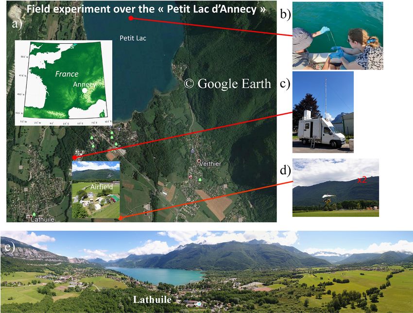
10914                                                      P. Chazette et al.: Water isotope profiles in Alpine lake (L-WAIVE)

Figure 1. Geographical location of L-WAIVE. The different pictures give a view of the environment where the measurements were per-
formed and of the instrumented platforms used: (a) location of the experiment, (b) lake water sampling from a boat, (c) instrumented van,
(d) instrumented ultra-light aircraft, and (e) panoramic view from UAV showing the location of Lathuile, as well as the Roc des Boeufs to
the left, the Tournette summit to the right, and the “Petit Lac” in between.

   During ascent and descent, the Airborne Lidar for At-               tween ∼ 1 and 2 h, depending on flight conditions, with a
mospheric Studies (ALiAS) aboard ULA-A was pointing                    cruise speed around 85–100 km h−1 . The ULA location was
sideways to directly derive the aerosol extinction coefficient         provided by a GPS and an Attitude and Heading Reference
(Chazette et al., 2007; Chazette and Totems, 2017). For the            System, which are part of the MTi-G components sold by
exploration of the valley at a cruising altitude between 3.5           XSens.
and 4.5 km a.m.s.l., ALiAS was pointing to the nadir. The
combination of both flight sequences thus allowed to survey            3.1.1   ULA-A
the three-dimensional structure of the lower troposphere over
the lake and its surroundings. The individual flight character-        Rayleigh–Mie lidar
istics (time, maximum altitude, type of exploration) are pre-
sented in Appendix B for the two ULA (Tables B1 and B2                 ALiAS was especially developed by LSCE as an airborne
for ULA-A and ULA-IC, respectively).                                   payload dedicated to sample the atmospheric scattering
                                                                       layers and then the vertical structures of the atmosphere
                                                                       (Chazette et al., 2012, 2020). It emits a pulse energy of
3     Instrumental setup on each platform                              30 mJ in the ultraviolet at 355 nm with a 20 Hz pulsed
                                                                       Nd:YAG laser (ULTRA) manufactured by QUANTEL™
This section provides a detailed description of the payloads           (https://www.quantel-laser.com/, last access: 5 July 2021).
on all platforms deployed during L-WAIVE. The periods of               The acquisition system is based on a PXI (PCI eXtensions
operation of each measurement platform are given in Ap-                for Instrumentation) technology. The receiver contains two
pendix A.                                                              channels for the detection of the elastic backscatter from
                                                                       the atmosphere in the parallel and perpendicular polarization
3.1    Airborne payloads                                               planes relative to the linear polarization of the emitted radia-
                                                                       tion. The native resolution along the line of sight is 0.75 m, it
We used two Tanarg 912 XS ULA from the company Air                     is degraded here to 100 m during the data treatment to im-
Création (Chazette and Totems, 2017). For each ULA (ULA-               prove the signal-to-noise ratio. The wide field of view of
A and ULA-IC), the maximum total payload is of approxi-                ∼ 2.3 mrad ensures a full overlap of the transmit and receive
mately 250 kg, including the pilot. Flight durations were be-          paths close to 200–300 m from the emitter.

Atmos. Chem. Phys., 21, 10911–10937, 2021                                               https://doi.org/10.5194/acp-21-10911-2021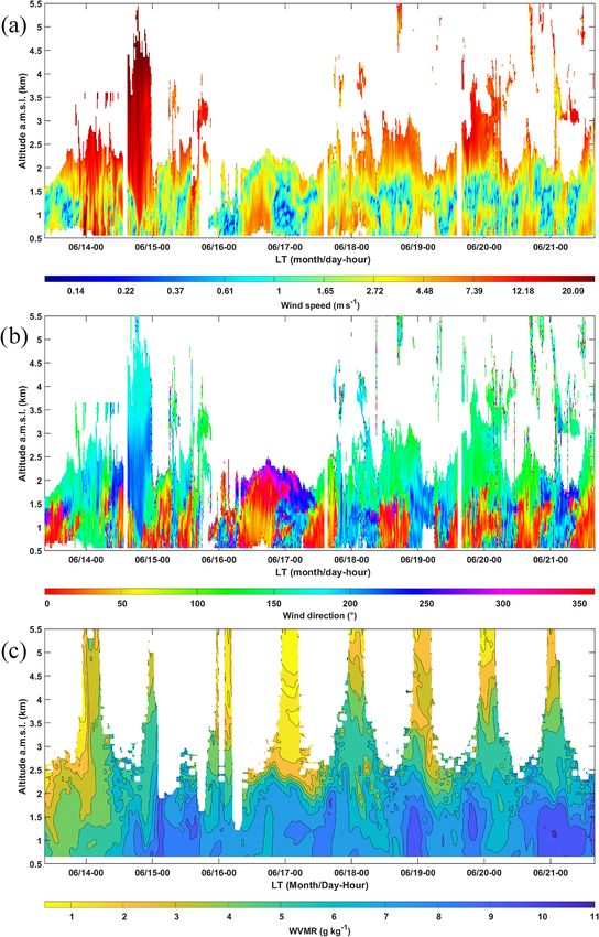
P. Chazette et al.: Water isotope profiles in Alpine lake (L-WAIVE)                                                                     10915

Figure 2. Example of a typical ULA flight plan performed during L-WAIVE (performed on 17 June 2019). (a) The flight track adopted
during the flight (blue dots for vertical profiling and red dots for horizontal exploration above the lake). DEM is the digital elevation model.
(b) Schematic representation of the measurement strategy adopted during L-WAIVE. Two types of sampling strategy are illustrated: red for
atmospheric sampling and green for cloud sampling. The purple arrows illustrate that the atmospheric sampling is performed during both
ascent and descent.

Meteorological probe                                                      of 0.25 hPa, the air temperature within an uncertainty of
                                                                          0.2 K and relative humidity (RH) within a relative uncer-
Part of ULA-A payload was a shielded meteorological probe                 tainty of 2.5 %.
VAISALA PTU-300 for measuring temperature, pressure,
and relative humidity. This probe measures the atmospheric
pressure, with a 1 min sampling time, within an uncertainty

https://doi.org/10.5194/acp-21-10911-2021                                                 Atmos. Chem. Phys., 21, 10911–10937, 2021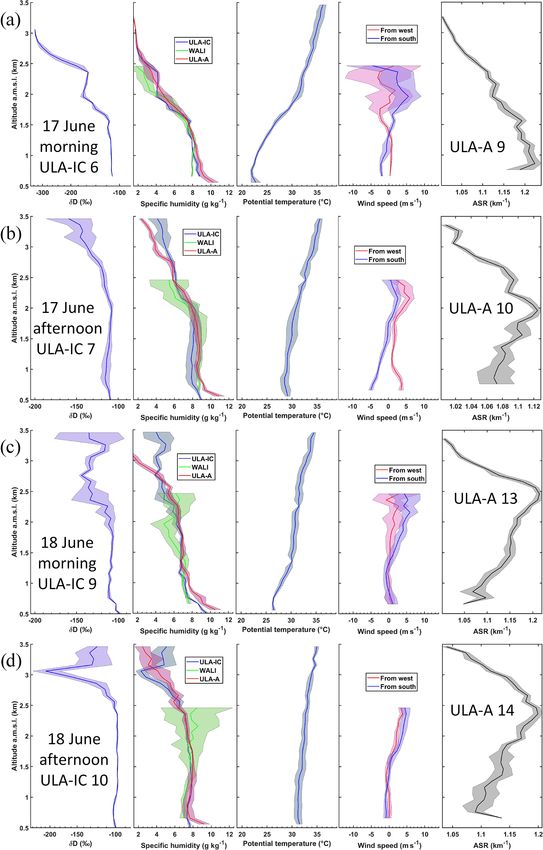
10916                                                    P. Chazette et al.: Water isotope profiles in Alpine lake (L-WAIVE)

3.1.2   ULA-IC                                                     the ULA. In order to sample droplets under the same condi-
                                                                   tions as those obtained on the ground, the CASCC fan was
CRDS water vapour isotope analyser                                 removed, and its inlet and outlet were prolonged with conver-
                                                                   gent and divergent high-density polyethylene (HDPE) cones
ULA-IC carried a CRDS water vapour isotope analyser                to ensure an isokinetic air sampling. All parts necessary to
(L2130-i, Picarro Inc., Sunnyvale, USA; ser. no. HIDS2254)         adapt the HDPE cones on the CASCC were made of plastic.
for the in situ measurement at about 5 Hz of the H16   2 O mix-    The flow through the probe must be steady and as turbulence-
ing ratio, and the isotope ratios δ 18 O and δ 2 H for H18
                                                        2 O and    free as possible. The design of these modified inlet and outlet
H2 HO, respectively. Water vapour was drawn into the spec-         was calculated to get a constant mass of water droplets per
trometer through an unheated inlet of 68 cm length (1/4 in         time unit through the probe aboard the ULA. The resulting
O.D. stainless steel with SilcoNert coating), pointing back-       probe was installed on the side of the ULA, where the flow
ward on the left side of the aircraft at a distance of 38 cm       was assumed laminar and allowed air sampling with a flow
from the CRDS. Pointing forward next to the vapour inlet, a        rate of 35 to 47 m3 min−1 , ahead of the motor exhaust. The
fast-response temperature and humidity probe (iMet XQ-2,           CASCC strings and inlet were pre-cleaned with deionized
InterMet systems, USA; ser. no. 61124) measured thermo-            water prior each flight and covered with a clean plastic bag
dynamic properties (T , RH, p with uncertainties of 0.3 K,         when not in cloud (especially during take-off and landing).
5 %, and 1.5 hPa, respectively) and GPS location at 1 Hz.          For a flight of 10 min inside a shallow cumulus cloud, the
The CRDS analyser was operated in flight mode, with a              probe typically collected 41 to 48 g of cloud liquid droplets
flow of about 150 sccm through the inlet maintained by a           corresponding to a liquid water content of 0.10 to 0.16 g m−3 ,
membrane pump (part no. S2003, Picarro Inc.). Pressure and         typical for such a cloud type (Herrmann, 2003).
water vapour mixing ratio were corrected using calibration
functions established at the FARLAB laboratory, University         3.2     Ground-based instrumentation
of Bergen, Norway. Raw measurements of the isotope pa-
rameters, expressed as δ values (see Appendix C), were cor-        The ground-based scientific facility hosted by the technical
rected for the mixing ratio-isotope composition dependency         department of the city of Lathuile was mainly composed of
and calibrated across the campaign period following recom-         the Raman lidar WALI (Weather and Aerosol Lidar) and of a
mendations from the International Atomic Energy Agency             scanning Doppler lidar. WALI was embedded in the ground-
(IAEA; see Appendix D for details). Tests with a small bub-        based MAS (mobile atmospheric station; Raut and Chazette,
bler system during the campaign indicated an anomaly in the        2009). The UAV (unmanned aerial vehicle) was also operated
CRDS measurements during 18–20 June, partially affecting           from this site, close to the lidar.
two flights on the morning of 19 June and the first flight on
20 June. The anomaly was due to a saturated inlet system           3.2.1    Raman lidar
from condensate forming on the aircraft during a cloud sam-
pling flight on 18 June. Flight periods affected by inlet sat-     WALI has been developed at LSCE (Chazette et al., 2014)
uration effects were excluded from further analysis (see Ap-       based on the same technology as its precursor instruments
pendix D).                                                         LESAA (Lidar pour l’Etude et le Suivi de l’Aérosol Atmo-
   A time resolution better than 0.1 Hz was obtained for spe-      sphérique; Chazette et al., 2005) and LAUVA (Lidar Aérosol
cific humidity from the CRDS and iMet probe, providing a           UltraViolet Aéroporté, Chazette et al., 2007; Lesouëf et al.,
spatial resolution of 200–300 m in the horizontal direction,       2013; Raut and Chazette, 2009). It is a custom-made instru-
and 10–50 m in the vertical, assuming a typical horizontal         ment dedicated to atmospheric research activities.
speed of 85–100 m s−1 and ascent rate of the aircraft of about        The receiver of the lidar is composed of two distinct detec-
1–5 m s−1 . Due to more complex memory effects, the isotope        tion paths with a low full-overlap distance (∼ 150–200 m).
composition has lower effective time resolution (Sodemann          The first path is dedicated to the detection of the elastic
et al., 2017; Steen-Larsen et al., 2014). We use here 10 s av-     molecular, aerosols, and cloud backscatter from the atmo-
erage data for all parameters on ULA-IC from upward pro-           sphere (Rayleigh–Mie lidar path). Two different channels are
files, filtered for rapid elevation changes, defined as exceed-    implemented on that path to detect (i) the total (co-polarized
ing 1.0 hPa ascent or 1.0 hPa descent within 10 s.                 and cross polarized with respect to the laser emission) and
                                                                   (ii) the cross-polarized backscatter coefficients of the atmo-
Cloud water collector                                              sphere. The second path, a fibered achromatic reflector, is
                                                                   dedicated to the measurements of the atmospheric Raman
A pre-cleaned Caltech Active Strand Cloud Water Collec-            scattering, namely the vibrational signal for nitrogen (N2
tor (CASCC, Demoz et al., 1996) was mounted on ULA-                channel) and water vapour (H2 O channel) and the rotational
IC, modified to efficiently collect cloud water at the relative    signal to derive the temperature (T channel).
cruising speed of the ULA (85 to 100 km h−1 ). The CASCC              During the entire experiment, the acquisition was per-
was modified to efficiently collect cloud liquid droplets from     formed for mean profiles of 1000 laser shots, leading to a na-

Atmos. Chem. Phys., 21, 10911–10937, 2021                                          https://doi.org/10.5194/acp-21-10911-2021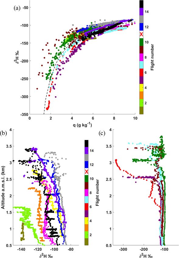
P. Chazette et al.: Water isotope profiles in Alpine lake (L-WAIVE)                                                         10917

tive temporal sampling close to 1 min. Rayleigh–Mie lidars          fore, the influence of the orography on the measurement is
are very efficient tools to detect scattering layers and then in-   assumed to be negligible here.
form on the vertical structures of the atmosphere (e.g. Platt,
1977; Berthier et al., 2006; Chazette et al., 2020). The water      3.3   Boat-borne payload: lake and atmospheric
vapour mixing ratio (WVMR) is retrieved with an absolute                  sampling
error less than 0.4 g kg−1 in the first 2 km above the ground
level (a.g.l.) (Chazette et al., 2014; Totems et al., 2019). The    The lake water surface and subsurface were sampled at the
calibration of the T channel is derived from the methodology        middle of the “Petit Lac” to measure water isotopes and
presented by Behrendt (2006) and leads to an absolute error         chemicals from the boat:
on the temperature lower than 1 ◦ C within the first 2 km a.g.l.      i. The lake water thermal stratification was monitored us-
The final vertical resolution is set to 15 m below 1 km a.g.l.           ing an EXO sonde, equipped with temperature, pres-
and 30 m above, and the temporal resolution is 0.5 h. In the             sure, pH, dissolved dioxygen, ion conductivity, and
following, a temporal resolution of 1 h is used.                         chlorophyll sensors. Profiles recorded in the middle of
                                                                         the “Petit Lac” (Fig. 1) once or twice per day (Table A1)
3.2.2   Wind lidar                                                       and showed that the thermocline was typically at a depth
                                                                         of about 7 to 13 m, in good agreement with previous
Wind profiles were measured using a scanning Doppler li-                 studies of the lake (Danis et al., 2003).
dar (Leosphere Windcube WLS100). It operates in the in-
frared (1.543 µm) with a low pulse energy (0.25 mJ) but a            ii. Subsurface water samples were collected at a depth
high pulse repetition frequency (20 kHz). The Doppler shift              of 2 m in HDPE-capped flasks. Surface water samples
due to the particles’ motion along the beam direction (ra-               were collected using a 30 × 30 cm silica glass plate im-
dial wind speed) is determined through heterodyne detection              mersed into water for a minute, then gently removed
followed by fast Fourier transform analysis. The acquisition             from water vertically (Cunliffe et al., 2013). The water
time was set to 1 s during the campaign. The pulse duration              falling from the plate in a continuous flow was not sam-
is 200 ns, corresponding to an axial resolution of 50 m given            pled; then, the dropwise water was collected in HDPE-
the pulse shape, with minimal and maximal ranges of 100 m                capped flasks. The surface microlayer samples were
and 7.2 km, respectively. The axial resolution can be low-               then collected by scraping the remaining water on the
ered to 25 m by reducing the pulse duration (100 ns) while               glass plates (using a rubber scraper) in amber glassware
increasing the pulse repetition frequency (40 kHz), which in             capped vials. All liquid water samples were measured
turn reduces the minimal and maximal range to 50 m and                   for isotopic composition (H18       2 16
                                                                                                       2 O, H H O) at FARLAB,
3.3 km, respectively. In practice, the maximum range is lim-             University of Bergen, according to established labora-
ited by the signal level. A minimum carrier-to-noise ratio (i.e.         tory procedures (Appendix D).
signal-to-background-noise ratio) of −27 dB is required to          iii. On 22 June, the CRDS isotope analyser was taken
keep the radial wind uncertainty (determined from the spec-              aboard the boat to sample a cross section in the atmo-
trum peak width) below 0.5 m s−1 . Therefore, observations in            spheric layer just above the “Petit Lac” through the lo-
the free troposphere are possible only when elevated layers              cation used for in situ sampling on the other days. This
of aerosols are present. Even in the boundary layer, several             made it possible to capture the isotope concentrations as
days of very low aerosol load occurred during the campaign,              a function of the distance from the shore and the depth
in which case the carrier-to-noise ratio threshold was low-              of the lake on that day. Water vapour isotope measure-
ered to −30 dB. With such a low carrier-to-noise ratio, the              ments were taken from an inlet at either ∼ 20 cm or
measurements must be considered with caution.                            ∼ 2 m above the water surface, while the iMet sonde
   Profiles of the three components of the wind vector                   measured temperature, relative humidity, and location.
were determined using the Doppler beam-swinging tech-                    We used 2.5 m of 1/4 in PTFE tubing and a 40 cm 1/4 in
nique originally proposed for Doppler radar (e.g. Koscielny              stainless steel tip on the first inlet, and about 1.5 m of
et al., 1984). Here, the measurement cycle includes one verti-           tubing with a 50 cm stainless steel tip. A flow rate of
cal beam, for which the radial wind is the vertical component            about 10 L min−1 was provided by an external mani-
of the wind vector, and four slanted beams (15◦ from zenith)             fold pump (N022AN, KNF, Germany) to either of the
in the cardinal directions to derive the two horizontal compo-           selected inlet lines. Post-processing and calibration of
nents of the wind. The uncertainty on the horizontal/vertical            water vapour measurements were done as for the air-
wind components is determined using the variability inside               craft data (Sect. 3.1.2).
averaging periods, possibly gathering several measurement
cycles. During the campaign, the Doppler lidar was posi-            3.4   Precipitation sampling
tioned in a wide valley (∼ 3 km at the observation site) with a
rather flat bottom, and the closest distance existing between       Precipitation samples were taken throughout the campaign
one of the slanted beams and an obstacle was ∼ 1 km. There-         period. The sampling device consisted in a pre-cleaned

https://doi.org/10.5194/acp-21-10911-2021                                        Atmos. Chem. Phys., 21, 10911–10937, 2021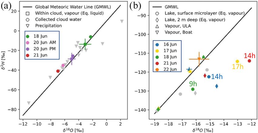
10918                                                     P. Chazette et al.: Water isotope profiles in Alpine lake (L-WAIVE)

HDPE funnel directly connected to a pre-cleaned HDPE
sampling bottle. The precipitation samples were manually
operated: after each precipitation event, the sample was
aliquoted into 1.5 mL glass vials with rubber/PTFE septa and
stored at 4 ◦ C prior to isotopic analysis, while the rest of the
sample was stored at −18 ◦ C. Precipitation sampling times
lasted from 20 min to several hours, depending on rainfall
rate.

4     Meteorological conditions during L-WAIVE

The synoptic and local weather conditions are analysed in the
following, helping with the subsequent interpretation of the
water vapour measurements in the lower troposphere over the
Annecy valley.

4.1    Synoptic conditions

During L-WAIVE, France was under the influence of two
main synoptic features, namely a pronounced trough over
Brittany and the British Isles and a high-pressure ridge over
northern Africa, sometimes extending across the Mediter-
ranean and all the way into eastern Europe. This weather sit-
uation is illustrated in Fig. 3 using the fifth European Centre
for Medium-Range Weather Forecasts Reanalysis (ERA5) at
0.75◦ horizontal resolution. This configuration caused a par-
ticularly strong pressure gradient over the western Mediter-
ranean for the period 12–15 June (Fig. 3a), flanked in the east
by an intense Libyan anticyclone, transporting warm air from
subtropics to midlatitudes. The ridge weakened and broad-
ened over the following days (16–19 June, Fig. 3b) before
strengthening again (20–23 June) as the Libyan high intensi-
fied (Fig. 3c).
   During the course of the campaign, the area of interest was
under the influence of warmer temperatures in the free tropo-
sphere linked with the high-pressure ridge at the beginning
and the end of the field campaign, and colder temperature
from 20 to 22 June. Since the experiment was conducted in a
valley, where ERA5 reanalyses are generally considered not
to be very accurate below the average altitude of the moun-
tains (∼ 2 km a.m.s.l. in our case), it is more informative to
use the measurements acquired during the field campaign
from the lidar and ULA to describe the evolution of mete-
orological variables (wind, humidity, temperature, pressure).

4.2    Insight on the local atmospheric conditions derived
       from lidars

During L-WAIVE, the temporal evolution of the scattering
layers, including clouds and aerosols, has been monitored us-
                                                                    Figure 3. ECMWF ERA5 temperature at 700 hPa (K, shading),
ing both the ground-based lidar (WALI) and the airborne li-         geopotential height at 700 hPa (gpm/1000, contours), and horizontal
dar (ALiAS). They provide insight into air masses transport,        winds at 700 hPa (black vectors) on (a) 14 June 2019 at 12:00 UTC,
weather situation, and local convection. For instance, such         (b) 17 June 2019 at 12:00 UTC, and (c) 22 June 2019 at 12:00 UTC.
a capability was used to improve our understanding of at-           The location of Lathuile is indicated with a grey dot surrounded by
                                                                    white.
Atmos. Chem. Phys., 21, 10911–10937, 2021                                            https://doi.org/10.5194/acp-21-10911-2021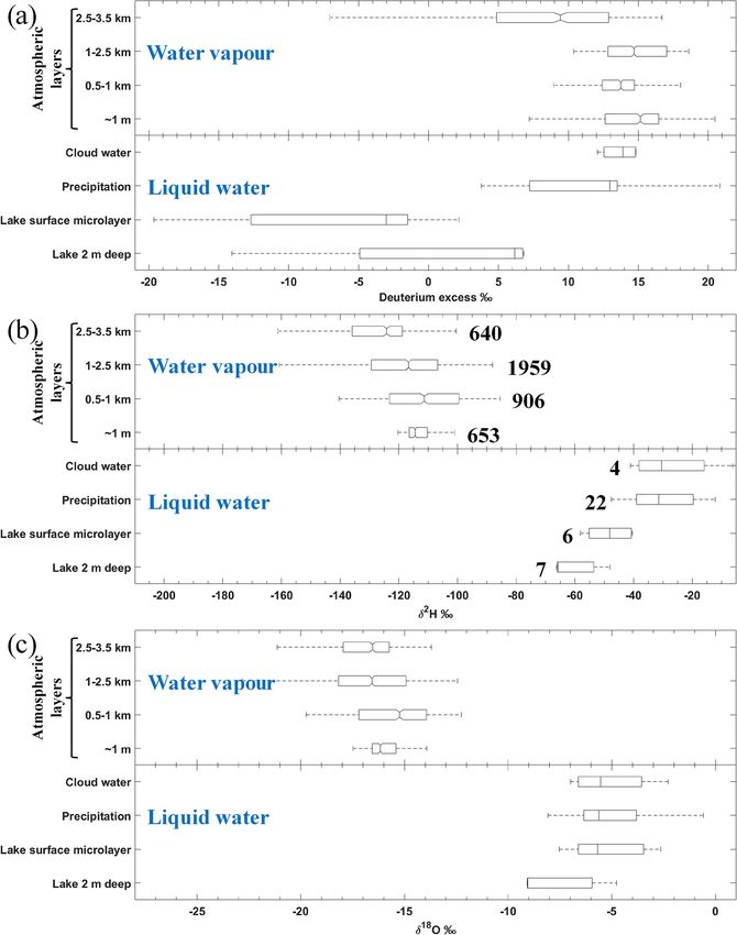
P. Chazette et al.: Water isotope profiles in Alpine lake (L-WAIVE)                                                          10919

mospheric circulation in complex situations such as extreme         are often observed at night, associated with nighttime downs-
heat wave phenomena (Chazette et al., 2017).                        lope winds, but may persist during days associated with
   Figure 4 shows the temporal evolution of the vertical pro-       heavy precipitation such as on 15 June 2019. The boundary
file of the aerosol (or cloud) apparent scattering ratio cor-       between high and low humidity of the free troposphere is also
rected from the molecular transmission (ASR, Fig. 4a) and           highlighted, especially at night when the lidar exhibits en-
of the linear volume depolarization ratio (VDR, Fig. 4b,            hanced sensing capabilities at higher altitude. For example,
Chazette et al., 2012). The vertical extension of aerosols in       high humidity is seen up to ∼ 4 km a.m.s.l. on the night of
the valley is highly variable over time as is the presence          17–18 June in agreement with what is highlighted in Fig. 4a.
and nature of clouds during the campaign. The strong diur-             The wind at the surface of the lake controls evaporation
nal cycle of ASR in the valley is tightly related to the slope      and turbulent surface fluxes and influences the thermal con-
winds and vertical stability associated with surface heating        vection, and cloud forcing influences the depth of the val-
and the forcing due to the presence of clouds. The depth of         ley boundary layer, allowing the mixing of water vapour in
the aerosol layer is the largest at the end of the afternoon        a layer of variable thickness over time. The influence of the
when the convection is the strongest in the valley, while it is     lake can therefore be seen up to altitudes of ∼ 4 km a.m.s.l.,
exhibiting a minimum around 11:00–12:00 LT when the val-            bearing in mind that the transition altitude to the free tropo-
ley winds reverse. The period was rather cloudy, with cloud         sphere is generally of the order of 2.5 km a.m.s.l. here. The
types and the rainy periods including thunderstorms being           altitude of this sharp transition is also linked to the average
indicated in Fig. 4a. In Fig. 4, we can clearly see the vertical    altitude of the mountains surrounding the measurement site.
updraft associated with clouds, which drives scatterers and         There are no big differences between day and night on this
water vapour towards higher altitudes, where there is a tran-       boundary. It should be noted, however, that there are sub-
sition to the free troposphere. The transition is between the       structures that can be characterized by wind shears at differ-
yellow and blue colours in Fig. 4a.                                 ent altitudes (Fig. 5b). A 0.5–1 km thick layer over the lake is
   Significant day-to-day variations of the aerosol layer depth     thus highlighted, which can be linked to the wetter structures
are thus observed during the field campaign which highlights        of Fig. 5c (in dark blue).
local, regional, and synoptic-scale transport of air masses
over the Annecy valley. At the beginning of the campaign
(mainly on 14 June), large VDR values are detected up to alti-      5     Water vapour isotope during L-WAIVE
tudes exceeding 7 km a.m.s.l. (Fig. 4b). These large VDR val-
ues are related to a large-scale Saharan dust transport episode     Water in vapour phase was sampled throughout the campaign
over the Lake Annecy valley favoured by the synoptic con-           in terms of mixing ratio of the main isotope and abundance
ditions on that day. These aerosols are progressively mixed         of isotopes H18          2 16
                                                                                   2 O and H H O. At the same time, liquid wa-
downward by subsidence, reaching the valley floor around            ter samples were taken from the surface of the lake, in the
00:00 LT on 15 June. The local wind in the valley is obvi-          clouds, and surface precipitation to obtain their isotopic con-
ously disturbed during stormy periods and during the episode        tents, and to place them in the context of the atmospheric wa-
of long-range dust transport on 14 June. The presence of            ter vapour of the lower troposphere. Water vapour was sam-
these aerosols at higher altitudes (up to ∼ 5 km a.m.s.l.) al-      pled in situ using a CRDS, whereas liquid samples, including
lowed the wind to be retrieved with the wind lidar above            precipitation, cloud water, and lake water, were analysed in
2 km a.m.s.l. (Fig. 5a–b).                                          the laboratory. Here, we report the isotope composition (see
   Strong southerly winds (in excess of 20 m s−1 above              interpretative framework in Appendix C) as δ values relative
3.5 km a.m.s.l.) were observed on 14 June in agreement with         to a standard (e.g. Gat, 1996).
the synoptic meteorological fields. Weaker winds, less than
5 m s−1 , are observed below 2 km a.m.s.l. for the entire pe-       5.1    Atmospheric in situ sampling
riod. The wind intensity does not show repetitive patterns
from one day to the next. Nevertheless, it is rather in the         In total, 15 flights with ULA-IC have been performed (see
course of the afternoon, when the wind comes from the north         Table B2), including 13 flights where the CRDS allowed a
to the south, that we have the strongest velocities in the plane-   representative sampling of δ 2 H and δ 18 O (Appendix D). The
tary boundary layer. Wind direction shows regular variations        isotope content δ 2 H observed during the flights ranged be-
(Fig. 5b), with winds directed towards the south during the         tween about −340 ‰ and −80 ‰ for flight altitudes up to
most of the afternoons. On the contrary, during the night and       ∼ 3.5 km a.m.s.l., as shown in Fig. 6a. For this figure, we
the first part of the morning, winds are directed towards the       considered ascending and level flight segments, and excluded
city of Annecy (north).                                             samplings with pressure increases larger than 1 hPa/10 s. As
   The vertical profiles of WVMR derived from the WALI              observed in earlier studies, the dataset is clustered along a
ground-based lidar are also shown in Fig. 5c. They highlight        typical mixing line in δ 2 H–q space (Noone, 2012; Salmon
highly variable water vapour in the first 2 km of the atmo-         et al., 2019; Sodemann et al., 2017). The end members of
sphere, as is the case with wind. Generally higher WVMRs            the mixing lines show substantial day-to-day variations, from

https://doi.org/10.5194/acp-21-10911-2021                                         Atmos. Chem. Phys., 21, 10911–10937, 2021
10920                                                        P. Chazette et al.: Water isotope profiles in Alpine lake (L-WAIVE)

Figure 4. Temporal evolution of (a) the aerosol scattering ratio (ASR) where the shaded areas correspond to the presence of clouds and
(b) the linear volume depolarization ratio (VDR) from 13 to 21 June 2019. The cloud type and rain location are indicated, as is the type of
the main aerosol structures identified by the VDR (orange/pink for dust on 14 June and other for pollution aerosols; clouds are in pink). Ns,
Ac, and Cu indicate nimbostratus, altocumulus, and cumulus clouds, respectively.

δ 2 H = −110 ‰ to −80 ‰ (∼ [−16, −12] ‰ for δ 18 O; not                     As shown in Fig. 6b–c, the vertical profiles of the iso-
shown) for the more humid end member (q > 8 g kg−1 ) and                 tope content δ 2 H show small variability with altitude below
from δ 2 H = −340 ‰ to −230 ‰ (∼ [−30, −20] ‰ for δ 18 O;                2 km a.m.s.l.; the greatest variability is observed in the first
not shown) for the drier end member (q < 3 g kg−1 ). It is               few hundred metres. In some cases, the profiles exhibit strong
important to keep in mind that both the variation in max-                vertical gradients at higher elevations, as seen between 2.5
imum flight altitudes and the meteorological situation can               and 3.6 km a.m.s.l. during five flights (flights 5, 6, 7, 9, and
contribute to variability.                                               10). The same patterns are observed on the vertical profiles

Atmos. Chem. Phys., 21, 10911–10937, 2021                                                 https://doi.org/10.5194/acp-21-10911-2021
P. Chazette et al.: Water isotope profiles in Alpine lake (L-WAIVE)                                                              10921

Figure 5. Temporal evolution of (a) wind speed (m s−1 ), (b) wind direction (0◦ is for north and 90◦ for east) obtained from wind lidar,
and the water vapour mixing ratio (WVMR) derived from the ground-based Raman lidar. White areas correspond to missing data caused by
detection limitations of the lidar (signal-to-noise ratio, presence of clouds).

https://doi.org/10.5194/acp-21-10911-2021                                            Atmos. Chem. Phys., 21, 10911–10937, 2021
10922                                                          P. Chazette et al.: Water isotope profiles in Alpine lake (L-WAIVE)

                                                                         air layer in a wind shear zone. We will discuss this vertical
                                                                         distribution of isotopes in more detail in Sect. 5.2.5.

                                                                         5.2   Cloud liquid water sampling

                                                                         Four relevant cloud water samples have been taken with
                                                                         the CASCC on 18, 20, and 21 June (Table A1). The iso-
                                                                         tope content of the cloud liquid water is shown in Fig. 7a
                                                                         (coloured circles). It is close to the global meteoric water line
                                                                         (GMWL) with corresponding d-excess values ranging from
                                                                         12.1 ‰ to 14.8 ‰. Equilibrium condensates were estimated
                                                                         from relevant water vapour isotope measurements during the
                                                                         time when the cloud samples were taken (Fig. 7a, coloured
                                                                         squares) using the fractionation factors of Majoube (1971),
                                                                         and air temperature measurements at cloud level, ranging
                                                                         between −4 and 1 ◦ C. It is worth noting that given poten-
                                                                         tial sources of uncertainty, the equilibrium condensate val-
                                                                         ues agree remarkably well with the cloud liquid water during
                                                                         18 June (green symbols) and the afternoon of 20 June (violet
                                                                         symbols). Overall, results here confirm that the cloud water
                                                                         droplets formed from equilibrium fractionation from ambient
                                                                         vapour. It is worth mentioning that such agreement between
                                                                         the completely independent sampling and measurement of
                                                                         vapour and cloud water supports the overall validity of (i) the
                                                                         cloud water sampling protocol, (ii) the airborne vapour iso-
                                                                         tope measurements, and (iii) the consistency of the calibrated
                                                                         water isotope dataset derived from the L-WAIVE campaign.

                                                                         5.3   Precipitation liquid water isotope composition

Figure 6. Overview of airborne water vapour isotope measure-             In total, 28 precipitation samples, of which 22 are unique,
ments. (a) Isotope content δ 2 H (‰) vs. specific humidity (g kg−1 ).    have been taken during the campaign, with sampling times
The mean mixing lines is computed following Noone (2012) with            lasting from 20 min to several hours, depending on rainfall
an end point q = 1.37 g kg−1 and δ 2 H = −335 ‰, and reported us-        rate (Table A1). The isotope composition in rainfall ranges
ing a dotted black line. (b, c) Vertical profiles of δ 2 H (‰). Colour   from −11.2 ‰ to 2.2 ‰ in δ 18 O and −73.5 ‰ to 9.6 ‰ in
indicates flight number. Panel (c) was added to separately plot the      δ 2 H (Fig. 7a, grey triangles), with corresponding values of
profiles with strong vertical gradients. Isotope data are averaged at
                                                                         d excess between 3.5 ‰ and 20.8 ‰ (not shown). Even if
10 s intervals. The red cross associated with flight 11 indicates that
no data were relevant during that flight.
                                                                         evaporation effects from the sampling setup cannot be fully
                                                                         excluded, in particular for the samples with a sampling du-
                                                                         ration of more than 3 h, the consistency of duplicate samples
                                                                         indicate that the influence of sampling artefacts can overall
of δ 18 O (not shown) and even on the WVMR profiles de-                  be considered as limited. Notably, there is an overall corre-
rived from the meteorological probes aboard the two ULA.                 spondence between the isotope range observed in cloud wa-
The sharp gradients are not observed systematically, as in the           ter samples and in a majority of precipitation samples. Devi-
case of flight 15 (20 June), or may be present at a higher al-           ations of precipitation samples from the GMWL indicate po-
titude, not sampled by the flight.                                       tential below-cloud exchange processes between the falling
   Indeed, because of the cloud cover and depending on the               raindrops and the ambient water vapour, leading to an enrich-
wind conditions, ULA have not been able to fly in the free               ment of the precipitation in 18 O (Graf et al., 2019; Worden
troposphere on most days. However, this was possible for                 et al., 2007). We have noticed that samples taken between 12
flight 10, where a marked reduction of δ 2 H occurred just               to 15 June, and on 21 June are most enriched in 18 O, exhibit-
above 3 km a.m.s.l., while higher values of isotopic content             ing the higher values in δ 18 O and δ 2 H and a smaller d ex-
are seen at higher altitudes that match those below the transi-          cess. These samples are from rainfall events associated with
tion. The same behaviour was observed on independent mea-                local thunderstorms. The corresponding low d excess (even
surements of water vapour mixing ratio, which may suggest                negative, ∼ −8 ‰) of these samples may point to the partial
filamentation associated with differential transport of drier            evaporation of rain droplets during their fall.

Atmos. Chem. Phys., 21, 10911–10937, 2021                                                https://doi.org/10.5194/acp-21-10911-2021
P. Chazette et al.: Water isotope profiles in Alpine lake (L-WAIVE) 10923
Figure 7. δ 2 H − δ 18 O plots of liquid samples compared to the vapour isotope estimates. (a) Cloud water samples (circles), equilibrium
condensate (squares), and precipitation samples (grey triangles). (b) Equilibrium vapour from lake water samples at various depths (dots
and diamonds) compared to vapour isotope measurements from ULA-IC (upward triangle) and boat (downward triangle). Colour denotes
matching dates (in the blue boxes are the colour legends in dot representation). Grey colours show data where the vapour samplings are
not available. The times of the lake water sampling are indicated next to the dots with the same colours. The black line denotes the global
meteoric water line (GMWL).
5.4 Lake liquid water isotope composition a mean of 0.6 ‰ and a standard deviation of 8.2 ‰. While
some sampling artefacts cannot be fully excluded, the fact
that there are differences between the isotope contents at the
Evaporation from Lake Annecy is expected to be an impor-
lake surface and 2 m depth points to the impact of ongoing
tant source for the water vapour in the low troposphere above
evaporation that decreases with depth. We note that temper-
the Annecy valley. In order to link the atmospheric profiles
ature profiles taken within the lake show a typically strong
of water vapour isotopes to the lake as a moisture source,
thermocline below about 7 m depth during summer (Danis et
20 lake water samples (Table A1) were taken throughout the
al., 2003). Therefore, freshwater input from runoff and pre-
campaign within the lake–atmosphere interface layer (6 sam-
cipitation, and loss to evaporation are expected to primarily
ples), as well as close to 2 m depth (14 samples), and anal-
affect the warmer, upper mixed layer within the timeframe of
ysed for their stable water isotope composition. The average
the campaign.
isotope contents were found to be −8.3 ± 1.5 ‰ for δ 18 O
The range of equilibrium vapour for δ 2 H observed in lake
and −63.0 ± 6.0 ‰ for δ 2 H. To assess the isotopic balance
water for 16 and 17 June (Fig. 7b, blue and yellow dots)
between the lake water and the water vapour isotope compo-
matches to first order with the range of δ 2 H from ULA-
sition measured by ULA and boat, we calculated the equi-
IC. However, the δ 18 O in equilibrium vapour is substantially
librium vapour for the lake surface temperatures measured
higher than the measured vapour value. This pleads for a
during respective days (Fig. 7b) using the equilibrium frac-
kinetic (non-equilibrium) fractionation during lake evapora-
tionation factors of Majoube (1971).
tion. During 18 June (Fig. 7b, green dot), equilibrium vapour
Lake water samples taken close to the surface are expected
of the liquid samples has a lower heavy isotope content than
to be most affected by evaporation, causing deviations to the
observed by ULA-IC, pointing to the influence of other fac-
right from the GMWL along evaporation lines (enrichment in
18 O) and corresponding to a negative d excess. As a matter tors on either atmospheric or lake water composition on these
days. However, one should be rather cautious about this inter-
of fact, lake water samples clearly cluster on the right-hand
pretation, as the time of the lake water sampling (∼ 09:00 LT)
side of the GMWL (Fig. 7b, diamonds), whereas vapour data
was significantly different from the time of the flight (flight
from the ULA-IC (triangles) and the boat (downward trian-
9 of ULA-IC, ∼ 12:00 LT), while for 16 and 17 June, the
gle) are to the left, with a relatively consistent range of iso-
measurements were performed at the same time. It is worth
tope values. The corresponding d excess underline this re-
noting that Lake Annecy is fed by a catchment whose surface
sult for the six lake water samples from the lake–atmosphere
is 10 times larger than that of the lake via 10 main tributaries
interface layer, with values of the d excess ranging between
located on the lake periphery. The flows of its tributaries in-
2.2 ‰ and −19.6 ‰ and an average value of −6.3 ‰. For the
crease significantly in situations of heavy rain, which can
samples taken at a depth of 2 m (Fig. 7b, diamond symbols),
substantially influence the isotopic content of the lake dur-
the derived d excess showed less evaporation influence, with
https://doi.org/10.5194/acp-21-10911-2021 Atmos. Chem. Phys., 21, 10911–10937, 202110924 P. Chazette et al.: Water isotope profiles in Alpine lake (L-WAIVE)
ing the course of a year; however, on 17 and 18 June, no rain ences have already been noted when comparing the samples
was observed. in Fig. 7b. On 17 June, wind-forced evaporation phenom-
ena may therefore intervene which may explain at least part
of the assumed isotopic fractionation. On the other hand, on
6 Synthesis and discussion 18 June, we have seen that the water samples are hardly rep-
resentative for ULA measurements as they were taken early
During the two main sunny days of the field campaign (17 in the morning, before the sun lit up the valley. Around noon,
and 18 June), the evolution of isotope content profiles in the the structure of about 300 m observed at the bottom of the
low troposphere (up to 3.5 km a.m.s.l.) is analysed together δ 2 H profile (Fig. 8d) and found in the other data is certainly
with the other observations including lidar measurements. In strongly influenced by evaporation from the lake. It is sig-
a second step, we provide a statistical overview of all the nificantly attenuated in the afternoon due to vertical mixing
available data to compare the various samples from the lake linked to thermal convection. We observe an enrichment in
2 H in this layer compared to the rest of the vertical profile
water to the low troposphere, including clouds, and precipi-
tation. in the morning that may be due to the lake evaporation into
depleted air.
6.1 Vertical profiles in the low troposphere as observed
from ULA 6.2 Statistical overview of isotopic content from the
lake to the atmosphere
Figure 8 shows the vertical profiles corresponding to four co-
ordinated flights between the two ULA. These flights were The main atmospheric vertical structures are derived from
carried out in the late morning and afternoon during the two the profiles of potential temperature, aerosols, wind, and wa-
sunny days of the campaign, i.e. 17 and 18 June. The profiles ter vapour mixing ratio. We have therefore defined three lay-
were constructed by averaging the data over 100 m bins. This ers in the low troposphere: (i) between the lake surface to
operation makes it possible to improve the signal-to-noise ra- 1 km a.m.s.l., (ii) between 1 and 2.5 km a.m.s.l., and (iii) be-
tio and to evaluate the dispersion of the measurements as a tween 2.5 and 3.5 km a.m.s.l. The uppermost value represents
function of altitude (coloured areas in the figure). our altitude sampling limit. The first layer can be identified as
The vertical structures of the lower troposphere are well the lake boundary layer, the second layer is associated with
reproduced across all data types, showing the consistency the region of influence of the lake, below the altitude of the
of the isotopic profiles with the independent observations. surrounding mountains, and the third layer is the transition
The strong gradients on δ 2 H above 2.5 km a.m.s.l. are related towards the free troposphere influenced by the regional cir-
to the transition to the free troposphere and are confirmed culation. The location in altitude of these different layers ob-
by the lidar observations and meteorological measurements viously depends on the weather conditions and the time of
on the two ULA. Discrepancies appear between the specific day.
humidity measured from the two ULA on 18 June above Using the vertical layering introduced above, the overall
2.7 km a.m.s.l. (Fig. 8c). This can be explained by the pres- results for stable isotopes in water are summarized in Fig. 9
ence of a fractional cloud cover. The ULA-IC has crossed on a statistical basis selecting the highest-quality data. This
part of the cloud base which is at the interface with the free synthesis is presented in the form of whisker boxes for d ex-
troposphere. cess (Fig. 9a), δ 2 H (Fig. 9b), and δ 18 O (Fig. 9c). For each
In the morning, the atmosphere near the lake shows near- subfigure, the upper part depicted the statistical content of
surface stability over 200 to 300 m which deteriorates/mixes isotope in water vapour for each sampled altitude range in
away in the afternoon according to the potential temperature the atmosphere, while the lower part describes the same thing
profiles. A few hundred metres above the lake, the atmo- for liquid water samples collected from clouds, precipitation,
sphere is very stable on 17 June in the morning (Fig. 8a); and in the lake, at the interface and subsurface. For the at-
it then loses stability in the afternoon due to thermal con- mospheric water vapour, the sample number n is significant
vection (Fig. 8b). On the morning of 18 June, the stability (numbers given at the right of the whisker boxes in Fig. 9b),
is strong below 1.5 km a.m.s.l. (Fig. 8c) and approaches the and it makes sense to accurately assess the confidence inter-
neutrality above this altitude. In contrast to 17 June, an at- vals at 95 %. As the notches do not overlap from an atmo-
mosphere close to neutrality is observed in the afternoon on spheric layer to another, we can conclude, with 95 % confi-
18 June (Fig. 8d), which may favour vertical exchanges from dence, that the true medians do differ. Hence, we highlight
the lake surface to the free troposphere. An important dif- a significant variability in the stable isotope content of wa-
ference between the 2 d is also related to the surface wind ter vapour depending on the atmospheric layers previously
speed. Winds of the order of 5 m s−1 were present on 17 June, identified.
whereas they were close to null on 18 June. Therefore, signif- Between the surface of the lake and 2.5 km a.m.s.l., we
icant differences in water exchange between the lake and the find δ 18 O values are in the lower range to those recorded by
atmosphere can be expected between the 2 d. These differ- Craig and Gordon (1965) for evaporation over the Mediter-
Atmos. Chem. Phys., 21, 10911–10937, 2021 https://doi.org/10.5194/acp-21-10911-2021You can also read