Extreme heat in India and anthropogenic climate change - NHESS
←
→
Page content transcription
If your browser does not render page correctly, please read the page content below
Nat. Hazards Earth Syst. Sci., 18, 365–381, 2018
https://doi.org/10.5194/nhess-18-365-2018
© Author(s) 2018. This work is distributed under
the Creative Commons Attribution 3.0 License.

Extreme heat in India and anthropogenic climate change
Geert Jan van Oldenborgh1 , Sjoukje Philip1 , Sarah Kew1 , Michiel van Weele1 , Peter Uhe2,7 , Friederike Otto2 ,
Roop Singh3 , Indrani Pai4,5 , Heidi Cullen5 , and Krishna AchutaRao6
1 Royal Netherlands Meteorological Institute (KNMI), De Bilt, the Netherlands
2 Environmental   Change Institute, University of Oxford, Oxford, UK
3 Red Cross Red Crescent Climate Centre, The Hague, the Netherlands
4 Columbia Water Center, Columbia University, New York, New York, USA
5 Climate Central, Princeton, NJ, USA
6 Indian Institute of Technology Delhi, New Delhi, India
7 Oxford e-Research Centre, University of Oxford, Oxford, UK

Correspondence: Geert Jan van Oldenborgh (oldenborgh@knmi.nl)

Received: 19 March 2017 – Discussion started: 31 March 2017
Revised: 29 October 2017 – Accepted: 27 December 2017 – Published: 24 January 2018

Abstract. On 19 May 2016 the afternoon temperature               aerosols to diminish as air quality controls are implemented.
reached 51.0 ◦ C in Phalodi in the northwest of India – a new    The expansion of irrigation will likely continue, though at a
record for the highest observed maximum temperature in In-       slower pace, mitigating this trend somewhat. Humidity will
dia. The previous year, a widely reported very lethal heat       probably continue to rise. The combination will result in a
wave occurred in the southeast, in Andhra Pradesh and Telan-     strong rise in the temperature of heat waves. The high hu-
gana, killing thousands of people. In both cases it was widely   midity will make health effects worse, whereas decreased air
assumed that the probability and severity of heat waves in       pollution would decrease the impacts.
India are increasing due to global warming, as they do in
other parts of the world. However, we do not find positive
trends in the highest maximum temperature of the year in
most of India since the 1970s (except spurious trends due        1   Introduction
to missing data). Decadal variability cannot explain this, but
both increased air pollution with aerosols blocking sunlight     In India, the highest temperatures occur before the monsoon
and increased irrigation leading to evaporative cooling have     starts, typically in May or the beginning of June. In partic-
counteracted the effect of greenhouse gases up to now. Cur-      ular, daily maximum temperatures are very high during that
rent climate models do not represent these processes well and    time. In the arid areas in the northwest, afternoon tempera-
hence cannot be used to attribute heat waves in this area.       tures often rise into the high 40s. On 19 May 2016 tempera-
   The health effects of heat are often described better by      tures exceeded 50 ◦ C in a region on the India–Pakistan bor-
a combination of temperature and humidity, such as a heat        der. In Phalodi the temperature even reached 51.0 ◦ C, which
index or wet bulb temperature. Due to the increase in hu-        is India’s all-time record (see also Fig. 1a–c). The previous
midity from irrigation and higher sea surface temperatures       record, from 1956, was 50.6 ◦ C. The heat wave lasted 3 days,
(SSTs), these indices have increased over the last decades       with temperatures the days before and after the hottest day
even when extreme temperatures have not. The extreme air         within 1 ◦ C of that value.
pollution also exacerbates the health impacts of heat. From         Excessive heat can have a devastating impact on human
these factors it follows that, from a health impact point of     health, resulting in heat cramps, exhaustion, and life-
view, the severity of heat waves has increased in India.         threatening heat strokes. Children, the elderly, homeless
   For the next decades we expect the trend due to global        and outdoor workers are most vulnerable. Excessive heat
warming to continue but the surface cooling effect of            can also aggravate pre-existing pulmonary conditions,
                                                                 cardiac conditions, kidney disorders and psychiatric ill-

Published by Copernicus Publications on behalf of the European Geosciences Union.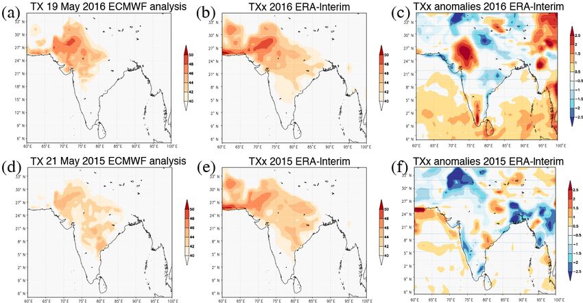
366                                    G. J. van Oldenborgh et al.: Extreme heat in India and anthropogenic climate change

Figure 1. (a) ECMWF operational analysis of the daily maximum temperature on 19 May 2016 (◦ C); (b) ERA-Interim highest maximum
temperature of the year, TXx, in 2016 (◦ C); (c) anomalies of TXx in 2016 relative to 1981–2010 (K). (d–f) Same as (a–c) but for 21 May 2015,
showing the heat wave in Andhra Pradesh and Telangana in 2015.

ness. High air pollution in India exacerbates many of                    While the trend in global average temperatures in general in-
these problems. According to newspaper reports, at least                 creases the probability of heat waves occurring (Field et al.,
17 heat-related deaths occurred in the Gujarat state, 7 in               2012; Stocker et al., 2013), this does not mean that heat
Madhya Pradesh and 16 in the state of Rajasthan, where the               waves in all locations are becoming more frequent, as fac-
highest temperatures were recorded during the heat wave                  tors other than greenhouse gases also affect heat. In this arti-
around 19 May 2016 (e.g. http://timesofindia.indiatimes.                 cle we investigate the influence of anthropogenic factors on
com/city/bhopal/Heat-stroke-kills-7-in-Madhya-Pradesh/                   the 2016 heat wave in Rajasthan, northwestern India, and the
articleshow/52403498.cms). Hundreds more people were ad-                 2015 heat wave in Andhra Pradesh and Telangana, eastern
mitted to hospitals in western India with signs of heat-related          India, which are shown in Fig. 1.
illness.                                                                    There are many different definitions of heat waves. Most
   The May 2016 temperature record followed a severe                     meteorological organisations have very different official def-
heat wave in Andhra Pradesh and Telangana in May 2015,                   initions, tailored to local conditions and stakeholders, usu-
which although not record-high in temperature had a large                ally based on maximum temperature and duration. In more
humanitarian impact with at least 2422 deaths attributed                 sophisticated definitions, the temperature and duration index
to the heat wave by local authorities (http://ndma.gov.in/               may be accompanied by humidity, as humid heat waves pose
images/guidelines/guidelines-heat-wave.pdf), more than half              a greater threat to human health (Gershunov et al., 2011). A
of which occurred in Andhra Pradesh. It is likely that the ac-           simple measure that includes this is the wet bulb temperature,
tual number of deaths is much higher as it is difficult to attain        which is the lowest temperature a body can attain by evapo-
figures from rural areas and deaths due to conditions that are           ration. It is therefore a measure of how well the human body
exacerbated by the heat (e.g. kidney failure, heart disease)             can cool itself via evaporation of sweat from the skin. As an
are often not counted (Azhar et al., 2014). Those directly               example, a temperature of 50 ◦ C with a relative humidity of
exposed to the heat including outdoor workers, the home-                 40 % has a wet bulb temperature of 36 ◦ C. This means it is
less and those with pre-existing medical conditions (e.g. the            equivalent to 36 ◦ C at 100 % humidity, which is a condition
elderly) constitute the majority of negative heat-related out-           in which it is almost impossible for the human body to cool
comes in India (Tran et al., 2013; Nag et al., 2009).                    itself.
   Naturally, the question was raised whether human-induced                 The Indian Meteorological Department (IMD) uses com-
climate change played a role in this record-breaking heat.               plicated definitions of heat waves and severe heat waves

Nat. Hazards Earth Syst. Sci., 18, 365–381, 2018                                   www.nat-hazards-earth-syst-sci.net/18/365/2018/
G. J. van Oldenborgh et al.: Extreme heat in India and anthropogenic climate change                                            367

based on single-day maximum temperature (imd.gov.in/               creasing. However, in the rest of India they find no significant
section/nhac/termglossary.pdf):                                    trend.
                                                                      As we were writing this article, Wehner et al. (2016) pub-
 1. heat wave need not be considered until the maximum             lished an investigation of the anthropogenic influence on the
    temperature of a station reaches at least 40 ◦ C for plains    May 2015 Andhra Pradesh and Telangana and June 2015
    and at least 30 ◦ C for hilly regions;                         Karachi heat waves using the 1- and 5-day mean daily max-
                                                                   imum of temperature and heat index. The latter also in-
 2. when the normal maximum temperature of a station is            cludes humidity. They find a low trend in the temperatures
    less than or equal to 40 ◦ C, the heat wave departure from     in Karachi, but a strong trend in Hyderabad. The heat index
    normal is 5 to 6 ◦ C and the severe heat wave departure
                                                                   has strong positive trends at both stations. This is confirmed
    from normal is 7 ◦ C or more;
                                                                   using Community Earth System Model (CESM) runs in the
 3. when the normal maximum temperature of a station is            current climate and a counterfactual climate without anthro-
    more than 40 ◦ C, the heat wave departure from normal          pogenic emissions. Again the difference is much more pro-
    is 4 to 5 ◦ C and the severe heat wave departure from          nounced in the heat index than in temperature.
    normal is 6 ◦ C or more;                                          In this article we mainly use a very simple definition: the
                                                                   highest daily maximum temperature of the year, TXx (Karl
 4. when the actual maximum temperature remains at 45 ◦ C          et al., 1999). This is related to the IMD definition of heat
    or more irrespective of normal maximum temperature,            waves but, rather than a simple dichotomy, it is a continu-
    a heat wave should be declared.                                ous measure that also describes the severity of the heat wave.
                                                                   It is thus also amenable to extreme value statistics. The 1-
   Four recent studies investigated trends in heat waves in In-    day length of the definition was chosen because of anecdotal
dia (Pai et al., 2013; Jaswal et al., 2015; Rohini et al., 2016;   evidence that the main victims in the 2015 heat wave were
Wehner et al., 2016). Using the IMD definitions, Pai et al.        outdoor labourers. Basagaña et al. (2011) also did not find
(2013) studied the trend in (severe) heat waves over India         a stronger effect from longer heat waves in Catalonia. In ur-
using station data from 1961 to 2010. In north, northwest          ban areas it is often found that longer heat waves have larger
and central India, some stations showed a significant increase     impacts, as the heat takes some time to penetrate the build-
in trend in (severe) heat wave days. However, other stations       ings of the most vulnerable population (e.g. Tan et al., 2007;
showed a significant decreasing trend in (severe) heat waves.      D’Ippoliti et al., 2010). To diagnose the causes of heat waves
The station of Phalodi in Rajasthan state, the site of the         we also consider the highest minimum temperature in May,
2016 record, showed a non-significant positive linear trend in     TNx.
the maximum temperature anomaly over the hot weather sea-             We mainly focus on the area of the 2016 record heat wave
son over 1961–2010. Overall, no consistent long-term trends        but also mention other regions, notably the location of the
were observed in heat wave days over the whole country.            2015 heat wave in Andhra Pradesh and Telangana. As society
   Another heat wave criterion considers the serious effects       is adapted to the weather of that location, we also show the
on human health and public concerns when the daily maxi-           anomalies relative to a long-term (1981–2010) mean of TXx.
mum temperature exceeds the human core body temperature            The second definition we use is the monthly maximum of the
(i.e. neglecting the cooling effects of perspiration). This cri-   daily maximum of the wet bulb temperature (Sullivan and
terion is used by Jaswal et al. (2015), who use a threshold        Sanders, 1974) as a measure that combines heat and humidity
of 37 ◦ C during the summer season March–June. Using data          and indicates how well the body can dissipate heat through
from 1969 to 2013, their findings indicate that long period        perspiration. This is related to, but not the same as, the heat
trends show an increase in summer high-temperature days in         index of Wehner et al. (2016).
north, west, and south regions and a decrease in north-central        We start with observed temperatures in 2015 and 2016
and east regions. This does not, however, give information         as well as trends in observed temperatures, with a detour
about the height of the maximum temperatures. In Rajasthan,        to the effect of missing data on these trends. Next we dis-
a maximum temperature of 37 ◦ C is a cool day in May.              cuss three factors that may have influenced heat waves be-
   More recently, Rohini et al. (2016) discusses the “exces-       sides global warming due to greenhouse gases: decadal vari-
sive heat factor”, which is based on two excessive heat in-        ability, aerosol trends and changes in humidity. The com-
dices. The first is the excess heat index: unusually high heat     bination is investigated further in global coupled climate
arising from a daytime temperature that is not sufficiently        models from the Coupled Model Intercomparison Project
discharged overnight due to unusually high overnight tem-          Phase 5 (CMIP5) and a large ensemble of sea surface tem-
peratures. The second index considered is the heat stress in-      perature (SST)-forced models. At the end we synthesise our
dex: a short-term (acclimatisation) temperature anomaly. Us-       findings into a qualitative overview of anthropogenic forc-
ing a gridded dataset from 1961 to 2013 they find, over a lim-     ings on the heat waves.
ited region in central and northwestern India, that frequency,
total duration and maximum duration of heat waves are in-

www.nat-hazards-earth-syst-sci.net/18/365/2018/                             Nat. Hazards Earth Syst. Sci., 18, 365–381, 2018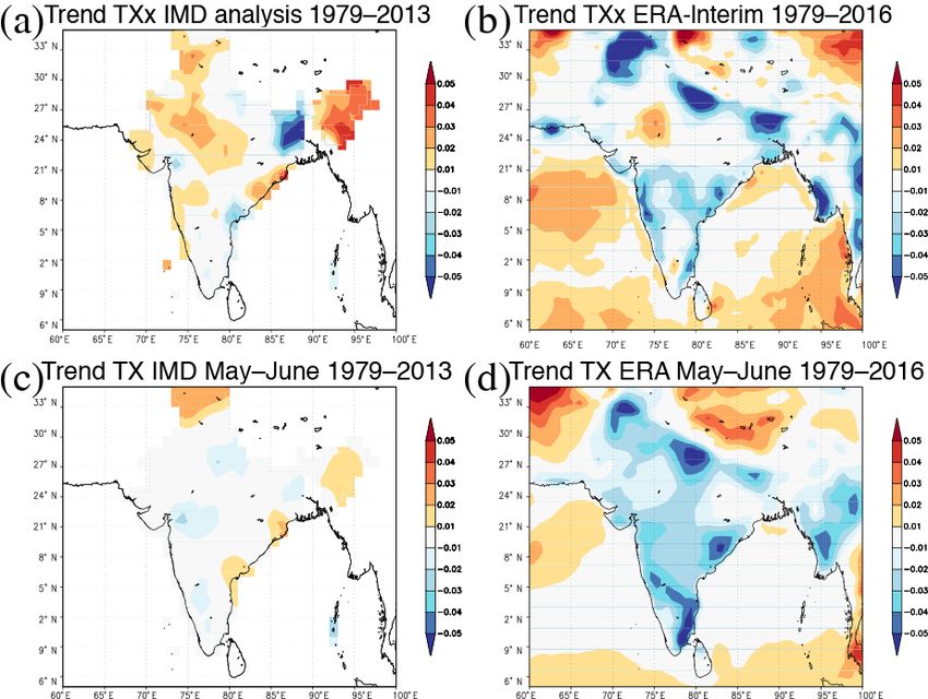
368 G. J. van Oldenborgh et al.: Extreme heat in India and anthropogenic climate change
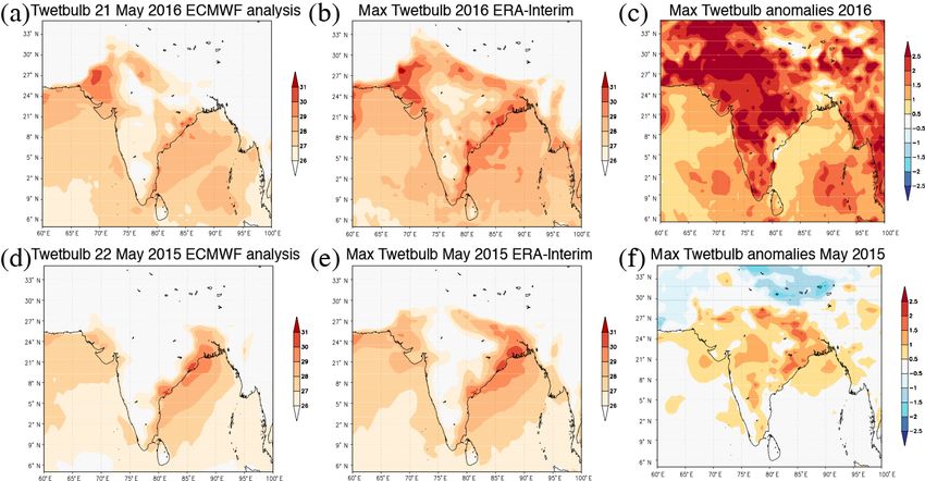
Figure 2. (a) ERA-Interim wet bulb temperature (T ) on 21 May 2016. (b) Monthly maximum of the wet bulb temperature in May 2016 (◦ C).
(c) Anomalies of the maximum wet bulb temperature in May 2016 (K), see text for details on the very high wet bulb temperatures in May
2016. (d–f) Same as (a–c) but for 22 May 2015.
2 Temperature observations 19 May 2016 and hence wet bulb temperatures were not ex-
tremely high. However, on other days during this heat wave,
such as 21 May, wet bulb temperatures reached more than
The record maximum temperature in India was observed on 30 ◦ C from this region to the coast (Fig. 2a and b), making
19 May 2016. The maximum temperature of the ECMWF heat stress a danger in outdoor labour. (Note that wet bulb
analysis for that day is shown in Fig. 1a. The analysis under- temperatures there were even higher in June. The east coast
estimates the heat somewhat relative to the in situ observa- also experienced similar wet bulb temperatures in 2016.) The
tions. For the northwestern part of India the temperature map wet bulb temperature was very high in 2016 compared to
of 19 May 2016 is comparable to the temperature map of other years (Fig. 2c). This could be due to the record warm
TXx for 2016 in ERA-Interim (Fig. 1b; Dee et al., 2011), Indian Ocean, due to the trend from global warming (Bind-
which only became available in September and has lower off et al., 2013) and the strong 2015–2016 El Niño (Fig. 3).
resolution. The highest temperatures occurred in and around However, we cannot exclude an inhomogeneity in the data
the northwest Indian state of Rajasthan and also in East Pak- from which it is computed, the ERA-Interim maximum and
istan. The largest anomalies were recorded slightly further dew point temperatures.
east, Fig. 1c, which was also mentioned in impact reports. In 2015, the wet bulb temperatures were somewhat higher
This heat wave did not have exceptional minimum temper- than normal in the region of the heat wave, but not by much
atures; the maxima of TN were recorded later in the month (Fig. 2f). Both the anomalies and values of the wet bulb tem-
and even further east. perature were higher further north along the coast in Odisha
The Andhra Pradesh and Telangana heat wave reached and West Bengal, with values over 30 ◦ C in the region of
temperatures of 44–45 ◦ C on 21 May 2015 (Fig. 1d and e). Kolkata (Fig. 2e). Only during the peak of the heat wave in
This temperature is not exceptional for other regions in In- Andhra Pradesh and Telangana were the wet bulb tempera-
dia, but it is about 1.5 ◦ C above the normal hottest afternoon tures higher there than in West Bengal, but not higher than in
of the year there (Fig. 1f). Minimum temperatures reach just Odisha.
over 1.0 ◦ C above climatology for one night, but twice larger
anomalies were recorded over the Ganges valley in 2015 (not
shown).
Next we consider the combination of heat and humid-
ity in the wet bulb temperature. The heat was very dry on
Nat. Hazards Earth Syst. Sci., 18, 365–381, 2018 www.nat-hazards-earth-syst-sci.net/18/365/2018/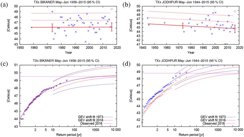
G. J. van Oldenborgh et al.: Extreme heat in India and anthropogenic climate change                                          369

                                                                 ima should be distributed according to a generalised extreme
    30.00
                                                                 value (GEV) function (Coles, 2001):
                                                                            "                 #
    29.00                                                                               x − µ 1/ξ
                                                                 F (x) = exp − 1 + ξ                ,                      (1)
                                                                                          σ
        1900   1920   1940    1960     1980    2000     2020
                                                                 where µ is the position parameter, σ is the scale parameter
Figure 3. March–May mean sea surface temperature in the north-   and ξ is the shape parameter. In order to incorporate possi-
ern Indian Ocean (EQ 30◦ N, 60–100◦ E) (◦ C). Source: ERSST v4
                                                                 ble effects of climate change we add the possibility that the
(Huang et al., 2015).
                                                                 position parameter changes linearly with time with a trend α:
                                                                 µ = µ0 + αt.                                                 (2)
3     Temperature trends                                         The uncertainties were estimated with a 1000-member non-
                                                                 parametric bootstrap procedure.
In line with global warming, the Indian annual mean temper-         The Bikaner series starts with some data around 1958 and
ature shows a clear trend (see, e.g. Hartmann et al., 2013).     has more or less continuous data starting in 1973. The se-
However, as pointed out by various studies (e.g. Pai et al.,     ries contains 11.5 % missing data in 1973–2015, mainly be-
2013; Rohini et al., 2016; Padma Kumari et al., 2007), this      fore 2000. We demand at least 70 % valid data in May–June
does not hold for the hot extremes. The highest maximum          to determine TXx; a higher threshold eliminates the obser-
temperature of the year, TXx, does not show a consistent sig-    vation of 49 ◦ C in 1973. The missing data will depress TXx
nificant trend over the whole country. In some parts of In-      somewhat as it may have fallen on a day without valid ob-
dia there is even a negative trend. This is shown in Fig. 4a     servation. This effect is stronger in the earlier part of the se-
for 1971–2012, with trends based on the gridded maximum          ries with more missing data. The lower TXx in the earlier
temperature analysis from IMD (Srivastava et al., 2008).         data leads to a spurious positive trend. For serially uncorre-
(Possible problems with gridded datasets in the study of ex-     lated data, the decrease from 30 % to almost 0 % missing data
tremes are discussed below.) The ERA-Interim reanalysis,         would give a spurious increase in probability of a factor 1.4,
which assimilates both station data and satellite data, shows    simply because at the beginning of the series the probability
similar though lower trends in TXx over the later period of      of observing the extreme would be only 70 %. The increase in
1979–2016 (Fig. 4b). The trend of the daily maximum tem-         the observed fraction from 70 to 100 % looks like an apparent
perature TX averaged over the whole pre-monsoon season,          rise in the probability of extremely high temperatures. This
which we take to be May–June, is even more negative in this      increase in probability corresponds to a spurious trend in
reanalysis (Fig. 4c).                                            temperature of roughly 0.1 K/10 yr here. However, this is not
   Focusing on the region of the 2016 heat wave, the pub-        the full story as the temperature values are strongly correlated
lic Global Historical Climatology Network Daily (GHCN-           from day to day: a heat wave usually lasts a few days. This
D) v3.22 dataset (Menne et al., 2016, 2012) does not con-        implies that even if the peak was not recorded, the chance is
tain the Phalodi series. There are two nearby stations with      high that one of the hot days is in the observed record. To
enough data to analyse. Bikaner (28.0◦ N, 73.3◦ E) has a rel-    take this day-to-day autocorrelation into account, a Monte
atively long and complete time series. It recorded a temper-     Carlo procedure using 100 time series of random numbers
ature of 49.5 ◦ C on 19 May 2016 according to newspaper          with the same mean, variance, autocorrelation and missing
reports – a record relative to the GHCN-D series. However,       data as the original was performed under the assumption that
the 2016 data are not publicly available. Jodhpur (26.3◦ N,      the missing data are randomly distributed over the series (we
73.2◦ E) does have 2016 data with a temperature of 48.0 ◦ C      verified that the missing data are not clustered). We find that
that day and 48.8 ◦ C on 20 May 2016. However, the histori-      the overestimation is 0.09 ± 0.03 K/10 yr for the Bikaner se-
cal series is more incomplete. We analyse both series.           ries when demanding at least 70 % valid data in May–June.
   Figure 5 shows the daily maximum temperature series for       For Jodhpur it is negligible, 0.00 ± 0.03 K/10 yr.
Jodhpur, albeit with some missing data, as well as the con-         Finally we are in a position to estimate the trends in TXx
tinuous series from ERA-Interim interpolated at Jodhpur’s        from the observed time series at the stations of Bikaner
coordinates. Together these data series indicate a heat wave     and Jodhpur. For this we determined TXx for each year
duration of 3 to 4 days, with 2 days (19–20 July) reaching       with enough data and fitted these to Eqs. (1) and (2) up
the “severe” category, according to the IMD heat wave def-       to 2015. The results are shown in Fig. 6. The fitted trend
inition. Note that before 1983, temperatures are recorded in     is 0.01 ± 0.28 K/10 yr (95 % uncertainty margins) at Bikaner
whole numbers, but in tenths of degrees Celsius after that.      and −0.15 ± 0.30 K/10 yr at Jodhpur. Neither is significantly
   Next we analyse the trend up to 2015. This excludes the       different from zero. They are in fact both slightly negative af-
heat wave itself, as that would give a positive bias. Accord-    ter subtracting the spurious trend due to the varying amount
ing to extreme value statistics theory, the May–June max-        of missing data discussed above. The absence of a positive

www.nat-hazards-earth-syst-sci.net/18/365/2018/                           Nat. Hazards Earth Syst. Sci., 18, 365–381, 2018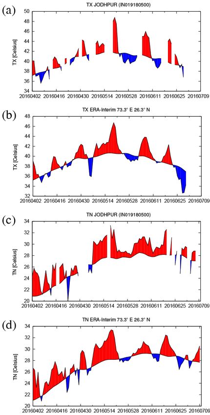
370                                 G. J. van Oldenborgh et al.: Extreme heat in India and anthropogenic climate change

Figure 4. (a) Trend in the highest maximum temperature in the IMD gridded daily analysis for 1979–2013 (K yr−1 ). (b) Same as in the
ERA-Interim reanalysis for 1979–2016. (c, d) Same as (a, b) but for the mean May–June maximum temperature trends.

trend remains when more valid data are demanded, e.g. 80 or         However, the location of Hyderabad Airport in the IND grid-
90 %.                                                               ded dataset of TXx only shows a trend in the period be-
   The return period diagrams in Fig. 6c and d show that the        fore 1980. Over 1973–2013 a linear trend is small and not
observed values have return periods of more than 40 years           significantly different from zero. Over 1979–2013 it is zero,
(95 % confidence interval); given the low number of data            whereas the ERA-Interim grid point has a significant nega-
points it is impossible to say how much more. It was a rare         tive trend over that period.
event at that location given the past climate.                         The return period of the 2015 event at Machilipatnam is
   We performed the same analysis for the heat wave in              quite low, about 15 years (95 % CI 9 to 40 years), which is
Andhra Pradesh and Telangana on 23–24 May 2015. The                 in agreement with the unexceptional temperature anomalies
station of Machilipatnam is close to the centre of the heat         in Fig. 1f. In fact, given that it covered less than 1/15th of
wave and has a relatively good time series for 1957–1958            the area of India one expects a heat wave with a return period
and 1976–2016, with 20 % missing data in the earlier part           like this almost every year somewhere in the country.
of the series, decreasing to less than 5 % in recent years.            We also considered the minimum temperature series at
The fit (not shown) for a cut-off of 70 % valid data in May–        these three stations, but they had too many missing data to
June gives a non-significant trend of 0.15 ± 0.40 K/10 yr.          be able to do a meaningful statistical analysis.
Repeating the procedure with 100 Monte Carlo samples                   The spurious trends due to changes in the fraction of miss-
with the same mean, standard deviation, autocorrelation             ing data may also explain part of the difference in trends be-
and missing dates but no trend gives a spurious trend of            tween the IMD observation-based TXx analysis and ERA-
0.19 ± 0.11 K/10 yr, so even this small trend is mostly due         Interim in Fig. 4. The IMD dataset is filled in by interpolat-
to the trend in missing values. Demanding 80 % valid data,          ing in time and/or space. An interpolated value will always
the observed trend becomes 0.02 ± 0.54 K/10 yr, of which            be smaller than the observations it is based upon, so the more
0.13 ± 0.07 is due to the trend in missing values.                  points that are interpolated rather than observed, the lower
   This agrees partially with the analysis of Wehner et al.         the extremes. This is not the case for the reanalysis, where the
(2016), who find no trend in Karachi, Pakistan, but a posi-         physical interpolation using a weather model of all available
tive trend in Hyderabad, Telangana, India, over 1973–2014.

Nat. Hazards Earth Syst. Sci., 18, 365–381, 2018                             www.nat-hazards-earth-syst-sci.net/18/365/2018/
G. J. van Oldenborgh et al.: Extreme heat in India and anthropogenic climate change                                              371

                                                                      waves in the rest of the world. For instance, for Australia,
                                                                      Perkins et al. (2014) show that the frequency and intensity
                                                                      in the likelihood of the extreme Australian heat during the
                                                                      2012–2013 summer had increased due to human activity.
                                                                      This is confirmed by Cowan et al. (2014), who find an in-
                                                                      creased likelihood in frequency and duration in the CMIP5
                                                                      ensemble in Australia. Sun et al. (2014) show that there is
                                                                      an increase in likelihood of extreme summer heat in East-
                                                                      ern China. The likelihood of a given unusually high summer
                                                                      temperature being exceeded in North America was simulated
                                                                      to be about 10 times greater due to anthropogenic emissions
                                                                      by Rupp et al. (2015), although the observations show no
                                                                      trends over the eastern half since the 1930s (Peterson et al.,
                                                                      2013). For central Europe, Sippel et al. (2016) use both ob-
                                                                      servations and models to show that the frequency of heat
                                                                      waves has increased. In a Swiss study, Scherrer et al. (2016)
                                                                      use over 100 years of homogenised daily maximum temper-
                                                                      ature data from nine MeteoSwiss stations. They show that
                                                                      over Switzerland the frequency of very hot days exceeding
                                                                      the 99th percentile of daily maximum temperature has more
                                                                      than tripled. Also, TXx in north-western Europe has a strong
                                                                      trend, as shown by Min et al. (2013). However, these stud-
                                                                      ies also show that in many regions, such as eastern North
                                                                      America and western Europe, there are large discrepancies
                                                                      between modelled and observed trends in heat waves.
                                                                         We propose three plausible mechanisms for the lack of a
                                                                      significant trend in TXx in India. The first is decadal vari-
                                                                      ability. The second is a masking due to a trend in aerosols,
                                                                      i.e. worsening air pollution that causes less sunshine to reach
                                                                      the ground and thus a surface cooling influence, especially in
                                                                      dry seasons. This happened in Europe up to the mid-1980s
                                                                      (e.g. van Oldenborgh et al., 2009) and there is evidence that
                                                                      this plays a role in India (Krishnan and Ramanathan, 2002;
                                                                      van Donkelaar et al., 2015; Padma Kumari et al., 2007; Wild
                                                                      et al., 2007). The third mechanism is an increase in irrigation
                                                                      (Ambika et al., 2016) that leads to higher moisture availabil-
                                                                      ity and hence increased evaporation, leaving less energy to
                                                                      heat the air. This has been shown to decrease temperatures in
                                                                      California (Lobell and Bonfils, 2008) and India (Lobell et al.,
                                                                      2008; Douglas et al., 2009; Puma and Cook, 2010). We in-
Figure 5. April–June daily maximum temperature time series from       vestigate each of these plausible mechanisms qualitatively in
(a) GHCN-D v3.22 observations at Jodhpur, the closest station to      the next sections.
Phalodi with publicly available data; and (b) ERA-Interim inter-
polated at the coordinates of Jodhpur (◦ C). (c, d) Same for the
daily minimum temperature. Departures from each dataset’s clima-
tology (1981–2010) are shown in red (positive) and blue (negative).
                                                                      4   Decadal variability
Days with missing data are left white.
                                                                      The Indian Ocean has very little natural variability, with the
                                                                      trend dominating (Fig. 3). El Niño clearly plays a role, with
                                                                      the 5-month lagged Niño 3.4 index explaining about a quar-
in situ and remote observations can also generate extremes            ter of the remaining variance after subtracting the trend (as a
when the ground temperature observations are missing.                 regression on the smoothed global mean temperature). How-
   We conclude that there are no significant trends for the           ever, there is no decadal variability visible, especially after
highest temperature of the year, TXx, in the regions with             the second world war when the quality of observations is
the record temperatures in 2015 and 2016. Instead, we find            higher. Considering well-known modes of decadal variabil-
near-zero trends. This is in contrast to most studies of heat         ity, the Pacific Decadal Oscillation (PDO) seems to cause

www.nat-hazards-earth-syst-sci.net/18/365/2018/                                Nat. Hazards Earth Syst. Sci., 18, 365–381, 2018
372                                   G. J. van Oldenborgh et al.: Extreme heat in India and anthropogenic climate change

Figure 6. (a) Observed TXx at Bikaner, Rajasthan, India (GHCN-D v3.22) with a GEV that shifts with time fitted (excluding 2016), de-
manding 70 % valid data in May–June. The thick line denotes µ and the thin lines µ + σ and µ + 2σ . (b) Same for Jodhpur. (c) Gumbel plot
of the fit in 1973 and in 2016 (central lines). The upper and lower lines denote the 95 % confidence interval. The observations are shown
twice, shifted up and down with the fitted trend. (d) Same for Jodhpur.

higher temperatures along the Indian coasts, but this is just          warning levels for unhealthy conditions of 150 µg per cubic
the effect of El Niño that is also visible in the PDO. The             metre (WHO, 2016). At ground level the pollution peaks in
Atlantic Multidecadal Oscillation (AMO) does not have tele-            the winter season under an inversion layer, with a secondary
connections to India. We conclude that decadal variability is          peak in the pre-monsoon season, just before the aerosols are
not a very likely cause of the lack of a trend in TXx over             washed out at the onset of the monsoon precipitation. The
India since the 1970s.í                                                effects on temperature are described by the aerosol optical
                                                                       depth (AOD), which includes the dimming effect of aerosols
                                                                       throughout the atmospheric column. The larger the AOD, the
5     Aerosols                                                         lower the fraction of sunlight that reaches the ground. In con-
                                                                       trast to the ground-level concentrations, the AOD peaks at the
It is known that aerosols contribute to solar dimming, e.g.            monsoon onset in June and is minimal in winter, when the
the reduction of solar radiation reaching the earth’s sur-             air pollution is confined to a thin layer near the ground. Re-
face (Streets et al., 2006; Wild et al., 2007). Krishnan and           cently, Govardhan et al. (2016) reported on the observed and
Ramanathan (2002) showed that the dry season trend is                  modelled differences between the high pre-monsoon (May)
lower than for the wet season and ascribed the difference              aerosol optical depth and much lower post-monsoon (Octo-
to the strongly increasing aerosol emissions. Padma Kumari             ber) AOD over India, most notably over both study regions
et al. (2007) quantified the average solar dimming in In-              of Rajasthan and Andhra Pradesh and Telangana (see their
dia and showed that the maximum temperatures over In-                  Fig. 5). Aerosol components contributing to the high pre-
dia are increasing at a much lower speed than expected                 monsoon AOD, though not well characterised, are thought
from global warming, while minimum temperatures did in-                to include significant amounts of black carbon, dust and sea
crease at higher speed. For Jodhpur the reduction in so-               salt. Note that all types of aerosols block part of the inci-
lar radiation reaching the surface between 1981 and 2004               dent sunlight and thus cool the surface, decreasing maxi-
was about −1 Wm−2 yr−1 in the predominantly cloud-free                 mum temperatures. Absorbing aerosols additionally heat the
pre-monsoon months, while for Visakhapatnam in Andhra                  lower atmosphere and are thought to affect the regional cli-
Pradesh the reduction was even more pronounced over these              mate through changes in cloudiness and tropical precipitation
decades with about −1.9 Wm−2 yr−1 .                                    (Krishnan and Ramanathan, 2002). The redistribution of the
   The people in South Asia and most of the inhabitants of             enhanced atmospheric heating by black carbon is still poorly
the cities in northern India suffer all year round from very           understood.
high levels of air pollution. Expressed in terms of particle
pollution (PM10 ) the annual mean may exceed the WHO 24 h

Nat. Hazards Earth Syst. Sci., 18, 365–381, 2018                                www.nat-hazards-earth-syst-sci.net/18/365/2018/
G. J. van Oldenborgh et al.: Extreme heat in India and anthropogenic climate change 373
Figure 7. (a) Mean May–June aerosol optical depth at 550 nm (AOD550) in the MACC reanalysis for 2003–2015. (b) Trend in AOD550
over this period (yr−1 ).
From ground-based observations it is reasonably well To conclude, there is strong evidence that the increase in
established that the AOD increased significantly before air pollution over India has given rise to a higher aerosol
the 2000s, decreasing the incoming solar radiation and there- optical depth in the pre-monsoon season, on top of year-to-
fore giving rise to a surface cooling trend that opposes global year fluctuations in dust load which dominates the AOD in
warming (Krishnan and Ramanathan, 2002; Padma Kumari this season. The consequent reduction in surface solar radia-
et al., 2007). To study the changes in AOD spatially over tion has resulted in a cooling trend in maximum temperatures
India we use the MACC reanalysis (Bellouin et al., 2013), during the pre-monsoon season, counteracting the warming
which is mainly constrained by MODIS AOD satellite ob- trend due to greenhouse gases. There is no evidence that this
servations. This reanalysis shows some decreases in aerosols trend has already reversed in the pre-monsoon period (Babu
in some areas since 2003, mainly in the northwest since the et al., 2013).
early 2000s (Fig. 7b). Spatially, there is some agreement be-
tween the area where AOD has started to recover over the
MACC period and the area with more positive trends in TXx 6 Moisture
(compare Figs. 4 and 7b).
It is however still unclear to what extent the record max- Soil moisture plays an important role in altering the parti-
imum temperature in May 2016 could be related to a start- tioning of the energy available at the land surface into sen-
ing downward trend in AOD. The AOD at end of May 2016 sible and latent heat fluxes. If the soil is dry, all incoming
still exceeded 1 over much of northern India (Fig. 7a), which energy is used for heating the air temperature. Therefore, ir-
is the highest in the world outside deserts. In the region of rigation can play an important role in heat waves, making the
Andhra Pradesh and Telangana the AOD still has a pos- soil wetter and therefore increasing the latent heat flux and
itive trend. A complicating factor for establishing trends reducing the sensible heat flux. This leads to lower tempera-
in anthropogenic aerosol in the pre-monsoon period is the tures but higher humidity (e.g. Lobell et al., 2008; Puma and
large interannual variability in dust load (Gautam et al., Cook, 2010). In a combined measure such as the wet bulb
2009). While dust storms might bring some relief by low- temperature, the effects counteract each other.
ering maximum temperatures, these storms also exacerbate As a measure for humidity we investigate the climatology
the health effects of heat waves. Also, high dust load re- and trends in dew point temperature, which is a function of
lated to lower maximum temperatures during daytime would specific humidity. In large parts of India, including the region
be accompanied during night by higher minimum temper- that is affected by the heat wave, there is an increase in dew
atures through a reduction in the outgoing longwave radia- point temperature in the pre-monsoon month of May in the
tion (Mallet et al., 2009), potentially compensating for the ERA-Interim reanalysis (Fig. 8a). This increase could be due
daytime dust-induced cooling. Because the observed total to expanded irrigation, although higher SST seems to play
AOD during the heat waves of May 2016 in Rajasthan and a role on the Pakistan coast. This agrees with Wehner et al.
May 2015 over Andhra Pradesh and Telangana were likely (2016), who find a significant increase in their heat index that
dust-dominated and not exceptionally low, the record maxi- also combines temperature and humidity, both in Karachi,
mum temperatures cannot be attributed to an onset of solar Pakistan, and Hyderabad, India.
brightening over these Indian regions. The trends in the highest May minimum tempera-
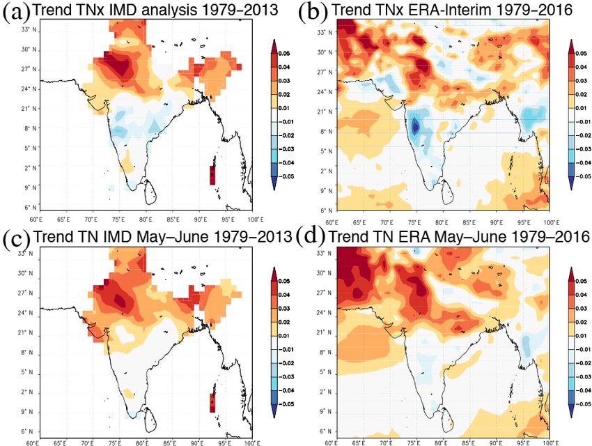
ture (TNx) show strong increases in TNx around New Delhi
and in the Punjab (Fig. 9a and b) and positive trends in the
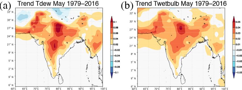
www.nat-hazards-earth-syst-sci.net/18/365/2018/ Nat. Hazards Earth Syst. Sci., 18, 365–381, 2018374 G. J. van Oldenborgh et al.: Extreme heat in India and anthropogenic climate change
Figure 8. Trend in (a) dew point temperature, (b) wet bulb temperature in ERA-Interim over May (K yr−1 ).
whole Ganges valley. The May averaged TN gives basically 7 Global coupled models
the same pattern (Fig. 9c and d). This gives additional sup-
port for the role of irrigation, as the regions with positive We next turn from observations and reanalyses to climate
trends are the areas where irrigation has increased. The in- models. First we analyse TXx in the CMIP5 ensemble (Tay-
creased evaporation and humidity are expected to increase lor et al., 2011) using the data from Sillmann et al. (2013)
nighttime temperatures as water vapour is a very effective at the grid point closest to 26◦ N, 73◦ E corresponding to
greenhouse gas (e.g. Gershunov et al., 2009). The increased the area of the 2016 heat wave in Rajasthan. The MIROC
humidity and wet bulb temperature in central India are not models were excluded as these have unrealistically high tem-
reflected in increased minimum temperatures there. We do peratures in arid regions, reaching almost 70 ◦ C here with
not know the reasons for this and note again that the redistri- large variability. A histogram of the trends in TXx in the
bution of the enhanced atmospheric heating by black carbon other 22 models over 1975–2015 is shown in Fig. 10. When
is still poorly understood. a model has Nens ensemble members these are each given
Also, during an extremely hot period, humidity is very im- weight 1/Nens so that each model is weighted equally. Nat-
portant for human health. In this sense, irrigation can have a ural variability (estimated from intra-model variability) and
negative effect on human health. The trend in humidity we model spread contribute about equally to the spread of the
found above is accompanied by a trend in wet bulb temper- results. The mean trend is lower than other semi-arid areas at
ature in May, see also Fig. 8b). A positive trend in wet bulb similar latitudes.
temperature means that for the same high temperature in the We compare this with the trends in the observed series at
past, the impact on people can be larger. The lack of a trend in Bikaner (corrected for the spurious trend due to the decreas-
the highest temperature of the year, TXx, therefore does not ing amount of missing data) and Jodhpur, as well as the near-
imply that there is no increase in the severity of the impacts est grid point in ERA-Interim. For reference we also show
of heat waves. the trend in the IMD TXx analysis, which is much higher
The humidity of the pre-monsoon season has increased in but has not been corrected for the varying fraction of missing
large parts of India. Wehner et al. (2016) show that humidity data and hence interpolation.
increases due to rising SSTs. Another factor is the increase The only two ensemble members with a negative trend are
in irrigation in India over the last decades; the inland re- from the CSIRO Mk3.6.0 and CCSM4 climate models. Other
gions with the largest humidity increases in Fig. 8a coincide ensemble members of these models have much higher trends,
with areas with increased irrigation (Lobell et al., 2008), who so we ascribe the low values to natural variability. None of
claim that the increase in irrigation already causes enough the models reproduces the negative trends in the observed
cooling to counteract greenhouse warming in northwestern series and ERA-Interim. The spatial pattern of the trend in
India. In all regions with increased irrigation the resulting in- TXx (Fig. 10b) also shows higher trends than observed over
crease in evaporation counteracts the temperature trend due most of South Asia and the western Bay of Bengal (Fig. 4).
to global warming, but the increased humidity also makes As the modelled trends are not compatible with the ob-
some impacts of heat waves more severe, e.g. by reducing served trends we did not use this ensemble for further anal-
the possibility of transpiration and increasing the night tem- ysis (similar problems were reported for the months of
perature (Gershunov et al., 2009). November–December in van Oldenborgh et al., 2016). The
uncertainties in the representation of the effects of aerosols
in the CMIP5 models are of course well known (see, e.g.
Bindoff et al., 2013, and references therein) and trends in ir-
Nat. Hazards Earth Syst. Sci., 18, 365–381, 2018 www.nat-hazards-earth-syst-sci.net/18/365/2018/G. J. van Oldenborgh et al.: Extreme heat in India and anthropogenic climate change 375
Figure 9. (a) Trend in the highest minimum temperature in May in the IMD analysis (Srivastava et al., 2008) for 1979–2015 (K yr−1 ),
(b) same as in the ERA-Interim reanalysis for 1979–2016; (c, d) same as (a, b) but for the trend in the May mean minimum temperature.
rigation have only started to be included after CMIP5 (Wada from the 2016 observations. We also looked at a third ensem-
et al., 2016). The large influence that these two misrepre- ble, climatological simulations of the years 1985–2014 using
sented anthropogenic factors have on trends in TXx in India observed SSTs and sea ice extent from the OSTIA dataset.
may well explain the discrepancy. These experiments are part of the weather@home project
(Massey et al., 2015) and use the Met Office Hadley Centre
atmosphere-only regional model HadRM3P at 50 km resolu-
8 Atmosphere-only model tion over the Coordinated Regional Downscaling Experiment
(CORDEX) South Asia region, nested within the global cir-
We furthermore used the distributed computing frame- culation model HadAM3P at 1.875◦ × 1.25◦ resolution.
work climateprediction.net to produce a very large ensem- Comparing the trend of TXx in the weather@home sim-
ble of atmosphere-only general circulation simulations of ulations in Fig. 11a to the observed and reanalysis trends
May 2016 in two different ensembles. The first ensemble (ac- in Fig. 4, we find that the patterns agree to some extent in
tual) simulates possible weather in the world we live in us- northwestern India where the 2016 heat wave occurred but
ing current greenhouse gases and observed Operational Sea disagree sharply along the eastern coast where the 2015 heat
Surface Temperature and Sea Ice Analysis (OSTIA) SSTs wave took place. We suspect that the two factors suppressing
and sea ice extent (Donlon et al., 2012) and a counterfactual the trend in TXx, aerosols and irrigation, are not well repre-
ensemble (natural) simulating possible weather in the world sented in this climate model (for example HadRM3p includes
that might have been without anthropogenic climate change. sulfate aerosols and the sulfur cycle but not black carbon).
As per Schaller et al. (2014), the anthropogenic signal was re- Nevertheless, we tentatively use this model for further anal-
moved from the SSTs used to force the counterfactual simu- ysis of the 2016 heat wave.
lations. As the uncertainty in estimating the pattern of anthro- Figure 11b shows the return periods of TXx in the region
pogenic warming is large, 11 different CMIP5 models and of the 2016 record in all three ensembles. The climatologi-
their multi-model mean were used to produce 12 different cal ensemble (orange) has a return period of a 51 ◦ C event
patterns of anthropogenic change in SSTs (see Table S20.2 occurring in May to be between 40 and 49 years (5–95 %
and Fig. S20.2 in Schaller et al., 2014), which we subtracted uncertainty range). This estimate compares well with return
www.nat-hazards-earth-syst-sci.net/18/365/2018/ Nat. Hazards Earth Syst. Sci., 18, 365–381, 2018376 G. J. van Oldenborgh et al.: Extreme heat in India and anthropogenic climate change
Figure 10. (a) Histogram of the trend in TXx (K yr−1 ) at the grid
point closest to 26◦ N, 73◦ E in the CMIP5 ensemble (excluding the
MIROC models). Ensemble members of the same model are down-
weighted so that each model gets a weight of 1. This is compared
with observations: the trends in Bikaner (corrected for varying miss-
ing data), Jodhpur and the nearest grid point of the ERA-Interim
reanalysis (left three bars). For reference the trend in the IMD grid- Figure 11. (a) HadAM3P model trend for 1986–2014 of TXx in
ded dataset without correction for varying missing data is also given May (K yr−1 ). Ocean points and areas not significant at p < 0.05
(rightmost bar). (b) Mean of trend in TXx (K yr−1 ) in the CMIP5 are shown as white. (b) Return time plots for TXx in May at the
ensemble 1971–2015, with historical experiments up to 2005 ex- grid box closest to Phalodi for “actual” 2016 simulations (red), “nat-
tended with the RCP4.5 2006–2016 simulations. ural” 2016 simulations (blue) and Climatology 1986–2014 simula-
tions (yellow).
periods obtained from the observational analysis. Compar-
ing this analysis with the simulations of the year 2016 under not make an attribution statement based on these model re-
current climate conditions (red curve) we find that the return sults.
period for an event of the same magnitude is only 1 in 7 to
10 years, while the return period in the “world that might
have been” (blue curve) is 1 in 20 to 30 years. 9 Discussion
In other words, the anthropogenic signal, as far as repre-
sented in the model, approximately trebled the likelihood of Contrary to most other regions of the world we find only lim-
the heat wave occurring, but the large-scale teleconnection ited evidence for positive trends in the highest temperature of
patterns as represented by the observed SSTs increased the the year (TXx) in India in observations and the ERA-Interim
likelihood of the event occurring by at least factor of 4. This reanalysis. The observed trends have a spurious component
suggests that the particular large-scale conditions of 2016 are due to a decreasing fraction of missing data: more heat waves
a major driver of the record being broken. In view of the still- were missed in the 1960s and 1970s than in the last decades,
large differences between the observed and modelled trends, giving the appearance of a positive trend. The lack of a trend
probably stemming from the 1SST from coupled models, is not due to natural variability in relatively short time series:
misrepresented aerosol effects and lacking trends in irriga- the upper bounds on the trends are smaller than we would
tion, the factor of about 3 increase due to anthropogenic expect from other regions around the globe. The absence of
emissions has a large model uncertainty. We can therefore a warming trend is also clear in the less noisy May–June
Nat. Hazards Earth Syst. Sci., 18, 365–381, 2018 www.nat-hazards-earth-syst-sci.net/18/365/2018/G. J. van Oldenborgh et al.: Extreme heat in India and anthropogenic climate change 377
mean of daily maximum temperatures over 1979–2016, both higher SSTs will result in an increase in humidity, leading to
in analysed observations and in the ERA-Interim reanalysis. higher heat wave impacts.
This lack of a trend implies that the recent record heat on Next we considered how trends in heat waves in India
19 May 2016 in Rajasthan of 51 ◦ C cannot simply be at- are represented in climate models. The global coupled cli-
tributed to global warming. It was a fairly rare event with mate models used for the IPCC Fifth Assessment Report
a local return period of more than 40 years. The heat wave (Stocker et al., 2013) have trouble representing the lack of
in Andhra Pradesh and Telangana around 22 May 2015 that trends in the highest temperature of the year. The surface
had a large human toll with thousands reported dead simi- cooling factors mentioned above do not seem to be well rep-
larly cannot be connected to the global warming trend. This resented (aerosols) or are not included (irrigation) in these
event was significantly less rare, with a return period of only models, which can therefore not be used for attributing the
about 15 years locally. As the area covered by the heat wave heat waves. An SST-forced model provides a better repre-
was less than 1/15th of the area of India, one expects a heat sentation of trends in northwestern India, but not along the
wave with such a return period almost every year somewhere east coast. Taken at face value, this model shows a factor of
in India. 3 increase in probability for the 2016 heat wave due to an-
We investigated qualitatively three factors that could have thropogenic factors, but with a large uncertainty again due to
counteracted the warming trend due to increased greenhouse uncertainties in the representation of aerosols and lack of ir-
gases. The first is decadal variability, for which we could rigation. This model also shows that the SST patterns of 2016
find no evidence in the observed record. Well-known modes made the heat wave more likely in 2016 than in other years by
of decadal variability also do not have an expression in pre- a factor of about 4, showing potential seasonal predictability
monsoon heat in India. of the event.
The second factor is air pollution: the thickening “brown This analysis also allows us to make qualitative projec-
cloud” over India prevents an increasing fraction of the sun- tions for the near future, up to 2050. Global warming is
light from reaching the ground, leading to a negative trend in set to continue until then with only minor differences be-
maximum temperatures. There is indeed evidence from both tween emission scenarios (Kirtman et al., 2013). SO2 emis-
ground-based and satellite observations that the aerosol op- sions averaged over India as a proxy for air quality are as-
tical depth has increased over the last decades. This increase sumed to peak around 2020 in RCP2.6, 2030 in RCP4.5, and
may have reversed lately in a small region of northern India 2040 in RCP8.5 (Nakicenovic et al., 2000) and decline after-
that is similar to the region with positive TXx trends. How- wards. With an expected doubling of India’s energy demand
ever, there is no evidence that the recent heat waves were up to 2040 (http://www.worldenergyoutlook.org/india), only
already made more likely by improved air quality. Large in- with prolonged and increasingly stringent air quality poli-
terannual variability in the dust load during the pre-monsoon cies would present-day air pollution levels be mitigated in
period will mask any long-term trend in anthropogenic pol- the coming decades (Cofala et al., 2015), so the peak date
lution levels for some time. is still highly uncertain. Irrigation is projected to increase,
We expect that the health and economic costs of the air though at a lower rate (Lobell et al., 2008), due to groundwa-
pollution will make it necessary to regulate air quality. Air ter depletion (Wada et al., 2010). Humidity increases due to
pollution exacerbates the health effect of heat waves. Besides higher SSTs will also continue.
the obvious benefits, a reduction in air pollution will lead to For maximum temperatures, this means that the main heat-
even higher maximum temperatures during heat waves. ing factor, greenhouse warming, will continue. The surface
The third factor is increased humidity, which can result cooling effect of aerosols up to now will turn into an extra
from more water availability, higher evaporative cooling and heating factor as the concentrations drop and the cooling ef-
hence lower maximum temperatures. There is evidence for fect of irrigation is expected to diminish in the future. The re-
increased humidity during the pre-monsoon season in much sult is projected to be a sharp increase in maximum tempera-
of India. Part of this is caused by higher sea surface temper- tures over the next decades. (A similar effect was seen in Eu-
atures, but the inland increases seem connected to increased rope in the 1980s when air pollution was reduced, van Old-
use of irrigation in that season. Lobell et al. (2008) argue that enborgh et al., 2009). Even though there has been no trend in
the increase in northwestern India has been strong enough TXx up to now, we expect a strong trend in the future.
to counteract the warming trend from greenhouse gases. Al- Even without a discernible trend in temperature, the im-
though increased evaporation suppresses maximum air tem- pacts of heat waves are considerable already. They have also
peratures, an increase in humidity does increase health risks, risen due to the increasing air pollution and humidity dur-
notably by making the cooling of the human body by evap- ing these heat waves, which both exacerbate the impacts of
oration of sweat from the skin more difficult and hence in- extreme heat on human health (Katsouyanni et al., 2009).
creasing the risk over overheating. Unlike the aerosol sur- The humanitarian impact of these heat waves was large, with
face cooling, evaporative cooling due to irrigation is expected 40 % of all extreme-weather-related deaths attributed to heat
to increase, albeit at a reduced rate. Both this increase and waves in 2016, which is the largest proportion of total deaths
of any type of extreme weather event (India Meteorological
www.nat-hazards-earth-syst-sci.net/18/365/2018/ Nat. Hazards Earth Syst. Sci., 18, 365–381, 2018378 G. J. van Oldenborgh et al.: Extreme heat in India and anthropogenic climate change
Department, Climate Research and Services, 2017). Experi- effect of aerosols to diminish as air quality controls are im-
ence in implementing heat wave interventions has shown that plemented, diminishing its impact on health. Humidity will
these deaths can be greatly reduced by straightforward mea- probably continue to rise as irrigation expands further, albeit
sures such as keeping parks and homeless shelters open on at a reduced rate, and SST rises. The combination will result
the hottest days and providing early warning of a forecasted in a strong rise in the temperature of heat waves. The high
heat wave (Fouillet et al., 2008; Tran et al., 2013). humidity will make health effects worse, whereas decreased
Changes in the vulnerability of the Indian population will pollution would decrease the impacts.
ultimately determine the impact of future heat waves. As In-
dian cities continue their rapid growth, the number of people
exposed to extreme heat due to inadequate housing and sus- Data availability. Most figures can be reproduced on the KNMI
ceptible to heat-related illness due to lack of access to drink- Climate Explorer (climexp.knmi.nl), albeit sometimes with newer
ing water or electricity is set to increase (Taru Leading Edge, versions of the datasets (please contact the authors if that
2016; Tran et al., 2013). They will also face hotter and more changes the results substantially; they should be robust against
improved data quality). Daily ERA-Interim data can be down-
humid heat waves.
loaded from http://apps.ecmwf.int/datasets/data/interim-full-daily/
levtype=sfc/. Daily TX and TN are computed from 6-hourly
maximum/minimum temperatures in the KNMI Climate Ex-
10 Conclusions plorer and are available at https://climexp.knmi.nl/select.cgi?field=
erai_tmax_daily and https://climexp.knmi.nl/select.cgi?field=erai_
An all-time Indian temperature record was recorded in tmin_daily. Maximum daily wet bulb temperature is similarly
Phalodi, Rajasthan, India, on 19 May 2016. We investigated computed from TX, dew point temperature and surface pres-
the influence of anthropogenic factors on the 2016 heat wave sure and is available at https://climexp.knmi.nl/select.cgi?field=
in Rajasthan and the 2015 heat wave in Andhra Pradesh and erai_twet_daily. The ECMWF operational analyses are not pub-
Telangana, which although not a record had a large humani- lic but the relevant ones can be provided by the authors
tarian impact. The 2016 event is rare, occurring at least once on request. The new ERA5 reanalysis (http://apps.ecmwf.int/
data-catalogues/era5/?class=ea) should give very similar results.
in 40 years, but the 2015 event is fairly common, occurring
For ERSST v4 (https://doi.org/10.7289/V5KD1VVF), we accessed
about once in 15 years.
the data through https://climexp.knmi.nl/select.cgi?field=ersstv4.
Considering a meteorological definition of a heat wave, the The IMD temperature analyses are not publicly accessible but are
highest temperature of the year TXx, we find no significant available at a charge for research purposes only, through http:
trend for either event. In agreement with earlier studies we //www.imdpune.gov.in/library/Data_Sale.html. For the GHCN-D
find positive trends in this measure only in a limited area in dataset (https://doi.org/10.7289/V5D21VHZ), we accessed the data
northern India, and these are overestimated due to a decrease through the KNMI Climate Explorer at https://climexp.knmi.nl/
in the fraction of missing data. The lack of trends is not due to selectdailyseries.cgi on 11 October 2017. It currently holds an up-
decadal variability, but the increase in aerosols from air pol- dated version. The GEV fitting routine is publicly accessible at the
lution and an increase in evaporation due to irrigation coun- KNMI Climate Explorer, and the code is open source. The MACC
tered the upward trend due to greenhouse gases. Both these reanalysis AOD data are available from http://apps.ecmwf.int/
datasets/data/macc-reanalysis/levtype=sfc/. The CMIP5 TXx data
factors also increase the health risks of heat waves, so the
are available from CCCMA at http://climate-modelling.canada.ca/
impacts have increased even if the temperatures have not. climatemodeldata/climdex/climdex.shtml and were used via the
The coupled climate models used in the latest IPCC report KNMI Climate Explorer at https://climexp.knmi.nl/selectfield_
do not represent the trends in the highest temperature of the cmip5_annual.cgi. The weather@home HadRM3P data are avail-
year correctly and hence cannot be used to attribute the trend able from https://www.climateprediction.net as batches 367 (ac-
or project the future. An SST-forced model does not perform tual), 370 (natural), 387 and 449 (climatologies actual and natural).
significantly better. (For the 2016 heat wave it does find that The data used for Fig. 11 are also available on the KNMI Climate
the large-scale climate conditions represented in the observed Explorer under “attribution runs”.
SSTs alone increased the likelihood by more than a factor of
about 4.) We therefore do not consider it possible to give an
attribution statement based on climate models for heat waves Competing interests. The authors declare that they have no conflict
in India as measured by maximum temperatures. of interest.
However, this may not be the most relevant definition.
Even without a discernible trend in temperature, the impacts
of heat waves are considerable and have risen due to their Acknowledgements. This research was done as part of the Raising
Risk Awareness project – a partnership between the World Weather
combination with increasing air pollution and humidity. Ex-
Attribution (WWA) Initiative and the Climate and Development
perience has shown that exposure and vulnerability can be Knowledge Network (CDKN) – and also supported in part by
reduced substantially with straightforward measures. the EU project EUCLEIA under grant agreement 607085. We
For the near-term future (up to 2050) we expect the trend would like to thank all of the volunteers who have donated
due to global warming to continue but the surface cooling
Nat. Hazards Earth Syst. Sci., 18, 365–381, 2018 www.nat-hazards-earth-syst-sci.net/18/365/2018/You can also read