Fate of the False Vacuum: Finite Temperature, Entropy, and Topological Phase in Quantum Simulations of the Early Universe
←
→
Page content transcription
If your browser does not render page correctly, please read the page content below
PRX QUANTUM 2, 010350 (2021)

          Fate of the False Vacuum: Finite Temperature, Entropy, and Topological Phase in
                             Quantum Simulations of the Early Universe
                      King Lun Ng , Bogdan Opanchuk, Manushan Thenabadu , Margaret Reid, and
                                              Peter D. Drummond *
             Centre for Quantum and Optical Science, Swinburne University of Technology, Melbourne 3122, Australia

                            (Received 11 October 2020; accepted 1 February 2021; published 24 March 2021)

                 Despite being at the heart of the theory of the “Big Bang” and cosmic inflation, the quantum-field-theory
              prediction of false vacuum tunneling has not been tested. To address the exponential complexity of the
              problem, a table-top quantum simulator in the form of an engineered Bose-Einstein condensate (BEC) has
              been proposed to give dynamical solutions of the quantum-field equations. In this paper, we give a numer-
              ical feasibility study of the BEC quantum simulator under realistic conditions and temperatures, with an
              approximate truncated Wigner phase-space method. We report the observation of false vacuum tunneling
              in these simulations, and the formation of multiple bubble “universes” with distinct topological properties.
              The tunneling gives a transition of the relative phase of coupled Bose fields from a metastable to a stable
              “vacuum.” We include finite-temperature effects that would be found in a laboratory experiment and also
              analyze the cutoff dependence of modulational instabilities in Floquet space. Our numerical phase-space
              model does not use thin-wall approximations, which are inapplicable to cosmologically interesting mod-
              els. It is expected to give the correct quantum treatment, including superpositions and entanglement during
              dynamics. By analyzing a nonlocal observable called the topological phase entropy (TPE), our simulations
              provide information about phase structure in the true vacuum. We observe a cooperative effect in which
              true vacua bubbles representing distinct universes each have one or the other of two distinct topologies.
              The TPE initially increases with time, reaching a peak as multiple universes are formed, and then decreases
              with time to the phase-ordered vacuum state. This gives a model for the formation of universes with one
              of two distinct phases, which is a possible solution to the problem of particle-antiparticle asymmetry.

              DOI: 10.1103/PRXQuantum.2.010350

                    I. INTRODUCTION                                   not yet verified. Quantum-field models are exponentially
                                                                      complex and impossible to solve directly.
   The evolution of the early universe described by infla-
                                                                         It is clearly not possible to repeat the start of the uni-
tion is now a standard model of cosmic evolution. This
                                                                      verse, so it has been proposed to verify the solutions
theory is widely accepted because of the observational
                                                                      experimentally. Such experiments would effectively be an
evidence including the cosmic microwave background
                                                                      analog quantum computer for the scalar-field dynamics
radiation (CMB) detected in all directions. This evidence
                                                                      of the universe. Here we note that the geometry should
points to a “Big Bang” origin as the beginning of the
                                                                      be multimode and have no boundaries, to allow free-
Universe. One of the building blocks is a quantum-field-
                                                                      space nucleation. The proposal for a suitable quantum
theory (QFT) model that explains the origin of the early
                                                                      analog computer uses a two-species Bose-Einstein conden-
universe and the observed temperature fluctuations in the
                                                                      sate (BEC) experiment in a one-dimensional uniform ring
CMB. These effects originated in Coleman’s theory of
                                                                      configuration, similar to those studied in several laborato-
quantum tunneling of a scalar quantum field in an initially
                                                                      ries [3–5]. The Bose-Einstein condensate has a modulated
metastable vacuum [1,2]. The validity of the thin-wall
                                                                      coupling between two spin components, which creates a
approximations used in this theory and later variations are
                                                                      local minimum in the effective phase potential. This allows
                                                                      an experimental study of models of false vacuum quan-
                                                                      tum tunneling in relativistic scalar-field theories, with an
  *
      pdrummond@swin.edu.au                                           engineered scalar-field potential.
                                                                         It is essential to also model the quantum simulator itself.
Published by the American Physical Society under the terms of
                                                                      Firstly, this provides insight into the quantum equations
the Creative Commons Attribution 4.0 International license. Fur-
ther distribution of this work must maintain attribution to the       themselves, even if only in an approximation. Secondly,
author(s) and the published article’s title, journal citation, and    it is necessary to understand the performance of the BEC
DOI.                                                                  quantum simulator, and its realization in the laboratory

2691-3399/21/2(1)/010350(22)                                   010350-1               Published by the American Physical Society
KING LUN NG et al.                                                                   PRX QUANTUM 2, 010350 (2021)

as far as possible. In this paper, we employ numerical         transition of the BEC from a metastable to a stable state
phase-space methods to simulate the quantum dynamics           is an ideal experiment for the investigation of Coleman’s
of the BEC quantum simulator under the conditions of           original idea. It simulates the relativistic scalar field as
laboratory experiments for up to 1024 modes. Earlier anal-     a relative phase between the spin components, with the
yses have verified a false vacuum tunneling, but have not       speed of light represented by the speed of sound in the
accounted for the effects of finite temperatures and Flo-        BEC. Related systems that have been studied include a
quet instabilities in such experiments. Our results show       BEC model of cosmic inflation [17], and using the pres-
that a momentum cutoff is essential, and that a low initial     ence of a seeded vortex within the condensate to initiate
temperature is required.                                       false vacuum decay [18].
   A feature of this scalar-field model is the existence of a      Here we treat a finite-temperature theory, as will occur
spontaneously broken discrete phase symmetry. This leads       in a real experiment. We utilize a variation of the Bogoli-
to nonlocal topological effects, which are uncovered using      ubov method [19] for treating the quantum initial state,
phase-unwrapping image-processing analysis on the data.        which employs a nonlinear chemical potential to eliminate
There are two distinct types of quantum vacua created with     divergences in the Bogoliubov theory [20]. We calculate
opposite phases. These are locally identical but globally      the effects of thermal noise on vacuum tunneling using the
distinct. Similar models have been employed as possible        truncated Wigner approximation, which has given success-
explanations of particle-antiparticle asymmetry [6–8]. We      ful quantum coherence predictions [10,21–25]. We show
show that such global topological effects can be quantified      that finite temperatures can enhance tunneling, and study
using the concept of an observational phase entropy, which     how tunneling rates are modified at different initial lab-
can both increase and decrease with time.                      oratory temperatures. These results include a momentum
   Each true vacuum created from the decay of metastable       cutoff to eliminate Floquet instabilities, and we show that
vacua can expand into a separate “universe” with differ-        a cutoff is essential by analyzing the effects of changing the
ent topological phases, creating domains of vacuum with        cutoff.
boundaries. The result of nucleation includes the tunneling       We also treat the dynamics and time evolution of the
rate, the fluctuations in density and temperature, and the      observable topological phase entropy, which has an intu-
collision of domain walls. All play an important role in the   itive, understandable interpretation. Tunneling events that
physical nature of the resulting universe formed. However,     form the vacuum are disordered, leading to a peak entropy
theoretical work so far relies on a number of assumptions      as time evolves. The entropy nearly reaches the max-
which have not been tested in an experiment. False vacuum      imum possible for an appropriate choice of space and
decay in zero space dimensions has been recently simu-         phase bins. As a result, there is a predicted dynamical
lated using a quantum computer [9], but this uses many         reduction with time in the topological entropy, as true vac-
orders of magnitude fewer qubits than are needed in a spa-     uum domains are formed. The final vacuum state is more
tial model. Here we simulate Coleman’s original model,         ordered, since the false vacuum is unoccupied. Domain-
including multimode spatial effects, although without the       wall formation is minimized at low temperatures, which is
gravitational effects required in a full cosmological theory.   important for cosmological interpretations [7], since it is
   The present paper describes a numerical simulation,         known that high-temperature domain-wall formation can
whose purpose is to evaluate the feasibility of an exper-      lead to anomalous CMB effects.
iment and to predict likely outcomes. We use the most
successful dynamical phase-space representation for long
times, which is the truncated Wigner (TW) approximation
to QFT [10,11]. This uses a 1/N expansion for N bosons,
and has had previous success in first-principles predictions     II. QUANTUM-STATE REPRESENTATION AND
of quantum dynamics in bosonic quantum fields. It gives                       HAMILTONIAN
correct predictions of tunneling in small bosonic quantum
systems with shallow potentials, by comparison to exact                            A. Field equations
number state and positive-P representation methods [12].          Bosonic quantum fields with internal degrees of freedom
Cosmological models also employ relatively flat potentials      [26–28] are used to describe the Higgs sector in the stan-
[13], so this is not unrealistic.                              dard particle model. Global symmetries of the Hamiltonian
   Previous work analyzed quantum bubble nucleation            are broken while creating the low-energy ground state or
using a 41 K BEC interferometer [14–16] at zero temper-        vacuum. The observation of the Higgs particle makes this
ature. This proposed a condensate containing atoms of          an important fundamental concept.
the same element with two spin components coherently              The theory of a metastable or “false” vacuum was devel-
coupled by a microwave field. The coupled BEC is ini-           oped by Coleman [1,2]. This used a simpler model, treating
tialized by a Rabi rotation into a metastable state, which     the fundamental quantum dynamics of a scalar quantum
decays into a stable state through quantum tunneling. The      field with nonderivative self-interactions and a Lagrangian

                                                         010350-2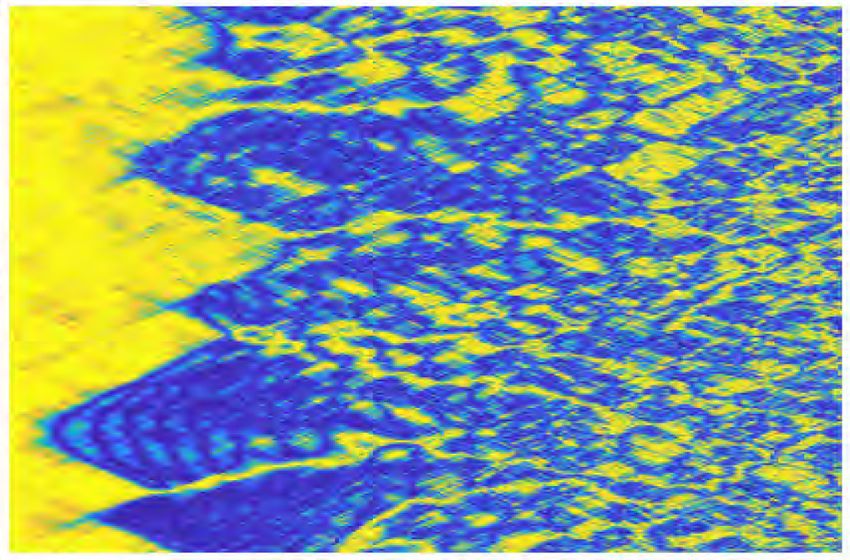
FATE OF THE FALSE VACUUM...                                                            PRX QUANTUM 2, 010350 (2021)

density (with a + − −− metric) of                               related to CMB spectral observations. A full quantum-
                                                                dynamical treatment of the location of domain walls is
                    1                                           needed. Our simulations show that at high temperatures,
                 L = ∂μ φ∂ μ φ − U (φ) .                 (1)    domain walls are prevalent. However, at low tempera-
                    2
                                                                tures, domain walls are restricted to universe boundaries
The local-field potential was defined to have two spatially       where they appear less likely to cause inhomogeneities
homogeneous, locally stable equilibrium states, φ = φ+          in the CMB spectrum. Observing domain walls in an
and φ = φ− . The first of these has a higher energy, with        experimental setting would help to verify or refute this
U (φ+ ) > U (φ− ). This is unstable to quantum corrections,     analysis.
and is expected to decay to the true vacuum, φ− . A char-
acteristic predicted to occur in such decays is that a true
                                                                         B. Approximations and interpretation
vacuum is formed by quantum tunneling at a particular
space-time point, and subsequently grows at the speed of           Since digital quantum computers are orders of magni-
light.                                                          tude too small, we propose to solve the equations using
   The dynamics of the evolution of the system is described     an analog quantum computer: a laboratory BEC quan-
by Heisenberg field equations of form                            tum simulator. In order to obtain insight into the expected
                                                                performance of the simulator, the dynamics of the BEC
                                                              system will be solved numerically, but with approxima-
                  ∂μ ∂ μ φ̂ + U φ̂ = 0.                 (2)    tions. Here, we give an outline of those approximations,
                                                                explaining where they will be expected to hold, and also
The fact that these are operator equations makes them           discuss the interpretation of the simulations.
effectively insoluble, apart from approximations. Even              An interesting consequence of all quantum models for
if all the eigenstates were known, as in some one-              the universe is that the entire universe is described as a
dimensional theories, there are exponentially many terms        single quantum state: there is no external observer. Quan-
[29] in an expansion of generic initial states.                 tum measurement theory in the conventional Copenhagen
   Coleman analyzed a scalar quantum-field theory of how         model requires an observer to collapse the wave function.
such a true vacuum would arise, given an initial metastable     As a result, there are foundational problems in interpreting
state. This model also predicted the formation of individual    the wave function itself. This leads to the question of what
early universe “bubbles.” Such theories can be extended to      can one identify in the simulation that will correspond to a
include gravitational effects, and have been used as a the-      universe?
ory of the early universe [30]. In these, the scalar field is       The numerical simulations of this paper give predictions
renamed the inflation field, and decay to a true vacuum           of the dynamics of the wave function for a model of the
causes an inflationary expansion [13], creating the “Big         universe according to a Hamiltonian treatment. As such
Bang.” More recent cosmological studies often focus on          the averages taken over the simulations provide the ensem-
postinflationary events [31], which are less sensitive to        ble predictions for the laboratory experiment if repeated
quantum fluctuations.                                            many times. An interesting question is whether or how a
   The observation of the Higgs particle and evidence for       particular laboratory realization can relate to a particular
CMB density fluctuations, confirms the importance of such         dynamical trajectory.
quantum-field-theory models. Yet the original false vac-            We use a mapping of the wave function to a Wigner
uum energies are thought to be many orders of magnitude         field distribution but with a simpler, approximate time-
greater than any possible experiment, possibly approxi-         evolution equation, which ensures a positive Wigner dis-
mately 1015 GeV [13]. The original event is also hidden         tribution throughout the dynamics. In this TW model,
from direct observation. In addition to such experimental       stochastic equations are written for complex amplitudes αk
problems, the quantum-field theory itself is exponentially       that represent modes k. These equations are solved numer-
complex, and cannot be solved exactly. As a result, the         ically, the quantum noise being modeled stochastically.
theory has mainly been analyzed using classical or per-         There is a direct correspondence between the observable
turbative approximations [32]. The inclusion of general         experimental moments of the field quadratures and the
relativistic effects further complicates the analysis.           moments of the real and imaginary parts of αk . The mea-
   It is important to have a better understanding of at least   sured quantity of interest is the particle number, which,
the simplest quantum-field-theory models. A feature of the       once operator ordering is taken into account, corresponds
model we use is that it possesses a spontaneously broken        to |αk |2 up to an error of order approximately 1. The values
discrete symmetry, which is known to provide a poten-           of |αk |2 encountered in the simulations are macroscopic,
tial solution to the particle-antiparticle asymmetry problem    and hence the difference between operator and simula-
[7]. Qualitative analysis of domain-wall formation at high      tion moments is negligible. In this sense, a probabilistic
initial temperatures has led to objections to this idea [8],    interpretation is possible, where the individual complex

                                                          010350-3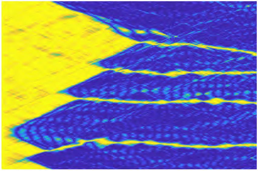
KING LUN NG et al.                                                                         PRX QUANTUM 2, 010350 (2021)

amplitudes’ trajectories correspond to an individual real-                        C. Two-species Hamiltonian
ization. Vacuum fluctuations may be considered as real               For a BEC system having two occupied hyperfine levels
events, and no additional collapse mechanism is required,        with mass m, the Hamiltonian of the coupled-field system
as discussed in greater detail in Sec. IV.                       includes an s-wave scattering potential [48]. It is impor-
   The dynamics of the TW distribution is approximate.           tant in our model that there is a strong mixing between
Even though the local evolution errors when using the            the two spin species, without a phase separation. This
TW method are of order 1/N where N is the num-                   requires that the interspecies interaction is minimized, and
ber of particles in each mode, these may grow during             is assumed to be zero here. There will be losses due to spin-
time evolution to create macroscopic errors at later times       changing inelastic collisions, but these dissipative effects
[12,33–35]. Such errors can increase during quantum tun-         are neglected. The size of such effects is not known for the
neling. The TW method cannot describe the formation              41
                                                                    K Feshbach resonance of interest. This provides a lim-
of macroscopic superposition states [36–40], or predict          itation on the accessible tunneling times, since the atoms
certain macroscopic Bell violations [41], because such           must tunnel before they are absorbed.
states cannot be described by a positive Wigner function.           A general two-species Hamiltonian includes both intra-
Quantum squeezing and entanglement can be described              and interspecies scattering. The interspecies scattering
however.                                                         length is often close to the intraspecies one, since differ-
   As it is a feasibility study, we do not give exact results,   ences in nuclear spin orientation do not strongly perturb
because the quantum-simulator experiment is intended to          interatomic forces. However, this can change dramati-
do this. Nevertheless, it is important to ask how reliable       cally at a magnetic Feshbach resonance. The required
the TW phase-space method is. The TW distribution has            tuning of the s-wave scattering interactions can therefore
been used to predict both squeezing and entanglement             be achieved with the external magnetic field chosen so that
in systems of large particle number. Comparisons have            cross-species scattering is suppressed. This is possible in
been made of TW and exact positive-P methods for the             41
                                                                    K, as well as in other isotopes like 7 Li.
dynamics of quantum squeezing in solitons [10,11,42],               In these cases, near the Feshbach resonance, one can
with excellent agreement between both methods and with           write the Hamiltonian as
experiments [21,22,43]. There is also good experimental
agreement for large-scale quantum BEC interferometry,

                                                                                                2
where fringe visibility decoherence times have been accu-                               Ĥ =           Ĥj + Ĥc .                (3)
rately predicted. In this regime, quantum entanglement                                          j =1
in the form of Schrödinger’s quantum steering has been
inferred based on the simulations, for states of up to 40 000
atoms [25].                                                      Here, writing  ˆj ≡ ˆ j (x, t) for brevity for the j th Bose
   Other studies treated quantum tunneling in driven             field, the individual spin-species Hamiltonians are
nonequilibrium systems, which showed agreement between
TW and exact methods for shallow tunneling potentials
                                                                                          ˆ j†
                                                                                               2 ∇ 2 ˆ  g †2 2
                                                                                                           ˆj
                                                                                                              ˆj ,
[12,33]. This agreement disappeared for deeper potential                  Ĥj =       dx −          j +                        (4)
                                                                                                2m       2
wells, which is more likely to lead to macroscopic super-
position states requiring negative Wigner distributions.
Another quantum-field system with metastable behavior             and the microwave coupling Hamiltonian, Ĥc , is
is the quantum solitonic breather [29,42], for which TW
methods have shown good agreement with conservation
laws [24] and both exact positive-P representation and                       Ĥc = −ν (t)       dx ˆ 2†    ˆ 1†
                                                                                                         ˆ1 +    ˆ2 .            (5)
integrable methods [44,45] during the early stages of
breather relaxation.
   While Coleman’s original model proposed a deep poten-         The components          ˆ j are the coupled-field operators cor-
tial, the models currently favored by many cosmolo-              responding to different nuclear spin states, and the sub-
gists do not. Instead, a shallow potential is thought to         scripts j , k = 1, 2 are the spin    indices. These operators
be more realistic in an inflationary universe [13]. As a          have commutation relations                        ˆ k x , t = 0 and
                                                                                                       ˆ j (x, t) ,
result, it is reasonable to use a relatively flat quantum-
field internal potential, with a large particle number. In         ˆ j (x, t) ,
                                                                                ˆ k† x , t = δjk δM (x − x). Here δM (x − x) is
this regime, the numerical simulation methods used here          a restricted δ function [49] that includes a momentum
appear reliable. Nevertheless, owing to the long time            cutoff, restricting the field to a lattice for numerical sim-
scales involved—and possible error growth [46,47]—the            ulation.
main goal is an experiment, regarded as an early universe           The coefficient g is the s-wave scattering interacting
quantum simulation.                                              strength between the atoms, which for a three-dimensional

                                                          010350-4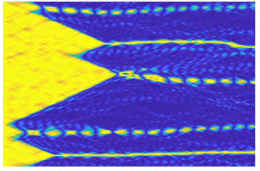
FATE OF THE FALSE VACUUM...                                                             PRX QUANTUM 2, 010350 (2021)

system, g3D , is given by

                               4π 2 a
                       g3D =           ,                  (6)
                                 m

where a is the s-wave scattering length.
   If the atoms are confined by a transverse harmonic trap
with frequency ω⊥ , where the transverse trapping energy
ω⊥ is much higher than the thermal energy, the Bose
gas reaches a one-dimensional regime [50]. In this regime,
the atoms are confined tightly within an effective s-wave
cross section As = 2π(l⊥ )2 , where l⊥ = /mω⊥ is the
transverse harmonic oscillator length [51–53]. The coeffi-
cient g for a one-dimensional system is hence expressed as
g = g3D /As , which gives                                        FIG. 1. The engineered potential for Eq. (9), with λ =
                                                                 1.0, 1.2, 1.5, showing a local minimum for λ > 1. Here ω0 = 1
                         22 a                                   for purposes of illustration.
                   g=          = 2aω⊥ .                  (7)
                         ml2⊥
                                                                 the relativistic field Eq. (2), where the√speed of light, c, is
We neglect microwave spontaneous emission effects, as             replaced by the phonon velocity, c = gρ 0 /m in the BEC.
these are very weak for such microwave transitions.                                                         ˆ j , which is equal
                                                                                                       ˆ j†
                                                                 The atom number density is ρ0 =
                                                                 for the two species.
        D. Stephenson-Kapitza pendulum term
                                                                    The potential equation is given by [16]
   The coupling ν describes a microwave field that rotates
the nuclear spin by resonantly coupling two hyperfine lev-
                                                                                                     λ2 2
els with a frequency separation of HF in the external                      U (φa ) = ω02 cos (φa ) +   sin (φa ) ,          (9)
magnetic field. This is modulated in time in order to induce                                          2
metastability using Stephenson’s concept of a modulated
                                                                                 √                    √
pendulum [54,55], later popularized by Kapitza [56,57].          where ω0 = 2 νgρ0 / and λ = δ 2gρ0 /ν. This poten-
The depth of the field potential in the metastable state is       tial can be varied by the experimentalist by changing λ, as
determined by the dimensionless variable δ.                      shown in Fig. 1, with a local minimum occurring if λ > 1.
   We work in a rotating frame such that this energy sepa-          It is known that instabilities can form due to effects
ration is removed from the Hamiltonian, using a different         caused by the modulation frequency and high-frequency
reference energy for each spin component. Here ν (t), the        phonon modes [61,62]. Such effects therefore require the
coupling strength between the spin components, is modu-          use of high enough modulation frequencies to move the
lated [54–58] as a sinusoidal time-dependent variable with       instability region above any physical cutoff in momentum.
an additional modulation frequency ω, so that                       We assume that there is a physical mechanism to remove
                                                                 high-momentum phonon modes. An example of this would
                  ν (t) = ν + δ ω cos ωt.                (8)    be the use of a spatially modulated potential to introduce a
                                                                 band gap. A second possibility is the use of a swept mod-
Provided the modulation is at a high frequency, this Hamil-      ulation frequency to reduce parametric gain by changing
tonian is equivalent to the Coleman model of a relativistic      the unstable momenta. Ultimately, as pointed out by earlier
scalar quantum field with an engineered quartic potential.        workers, the inverse scattering length provides an intrinsic
Here the phonon velocity corresponds to the speed of light       cutoff, ultimately at 1/a.
[14,16]. Modulation amplitudes are relatively large, so             An experimental mechanism to achieve this is via an
that the excitation is nearly bichromatic [59,60], or double     optically modulated trap potential. Instabilities were not
sideband.                                                        observed in our previous numerical simulations, due to the
   The result of including this term is an engineered poten-     use of a finite lattice that includes a momentum cutoff.
tial U (φa ) for an effective scalar field φa , which physically   An analysis of modulational instabilities in experiments
is the phase difference between the two coexisting Bose-          with larger numbers of modes and higher phonon momenta
Einstein condensates with phases φj . We define the atomic        is given in the Appendix, where typical parameters are
phase difference as φa = φ1 − φ2 − π , so that the false          presented.
vacuum is at φa = 0 and the true vacua are at φa = ±π .             We conclude that such instabilities are generally present,
In the limit of strong particle-particle repulsion, this obeys   but can be suppressed in the proposed experiment by

                                                           010350-5
KING LUN NG et al.                                                                           PRX QUANTUM 2, 010350 (2021)

                                                                      temperature. The condensate has thermal phonon excita-
                                                                      tions, which can change the tunneling time. These also
                                                                      induce phase fluctuations and finite temperatures in the
                                                                      effective scalar field.
                                                                         This is expected to give modified tunneling compared to
                                                                      a metastable quantum field without extra noise. Since the
                                                                      exact quantum state prior to the Big Bang is not known
                                                                      precisely, our goal here is to determine the effect of ther-
                                                                      mal noise on a laboratory experiment. Even this may not
                                                                      capture the full effects of evaporative cooling, which is a
                                                                      complex dynamical process [66].

                                                                                  A. Nonlinear chemical potential
                                                                         To model a finite-temperature experiment, we assume
                                                                      that the initial density matrix is in a grand canonical
FIG. 2. Example of a single trajectory decay to a true vacuum,        ensemble ρ̂GC at temperature T for j = 1, and a vacuum
starting in a 1D false vacuum initialized with finite-temperature      state for j = 2, so that
effects. The false vacuum is seen to decay to two distinct topo-
logical phases φa (x) for the true vacuum, indicated by yellow and                      ρ̂GC = e−β K̂ |0 0|2 .              (10)
light-blue regions. The bubbles of true vacuum expand in dimen-
sionless space x until they meet each other. At dimensionless        Here K̂ is the “Kamiltonian,” which includes a chemical
long time scales  t, the universes are separated by domain walls     potential to give a finite particle number in the thermal
of false vacuum, indicated by the color green. Dimensionless          state, so that
parameters are τ = 10−5 ,    ν = 7 × 10⁻³ , λ = 1.2, ω = 50, and

ρ
 = 200. The definition of the parameters is given in Sec. III C.
                                                                                          K̂ = Ĥ − μ N̂ ,                (11)

using high enough modulation frequencies combined with                where μ N̂ is the chemical potential for an initial popu-
a momentum cutoff, as shown in Fig 2.
                                                                      lation N̂ in one of the spin configurations. This can be any
                                                                      nonlinear function of N̂ [20], so that, including terms up to
 III. INITIAL STATE AT FINITE TEMPERATURE                             second order
                                                                                                       μ2
   Our initial state includes quantum and thermal fluc-                                μ N̂ = μ1 N̂ +         : N̂ 2 : .        (12)
tuations. We combine the Bogoliubov method [19] with                                                      2
the Wigner representation, so that both the initial ther-             The chemical potential
                                                                                              has no effect on the dynamics if
mal excitations and vacuum noise are taken into account.              ν = 0, since Ĥ , μ N̂ = 0. Such a nonlinear chemical
In this approximation, the system is assumed to have a
macroscopic condensate mean population Nc , with initial              potential is useful for describing thermal fluctuations in a
density ρc = 2ρ0 for one of the spin indices, say j = 1.              BEC. The utility of this method is that on linearizing the
Experimentally, this is produced using evaporative cooling            total Kamiltonian, K̂, the zero-frequency divergence of the
methods [63–65].                                                      Bogoliubov expansion [19] is eliminated with a suitable
   The ground-state field operator   ˆ 1 is nearly equal to           choice of the quadratic coefficient μ2 .
                                             √                            For number-conserving interferometric measurements
the square root of the condensate density, ρc , which is
assumed constant over the ring. This is valid for typi-               of relative phase, the initial coherent phase φc of the origi-
cal ultracold BEC experiments below threshold, provided               nal condensate is completely uncertain, and the system can
trapping potential noise is small. There are zero momen-              be viewed equivalently as having a statistical mixture of
tum divergences in applying the Bogoliubov expansion to               either condensate phase or atom number [20]. To allow
finite systems, which are removed here using a nonlinear               an expansion around a well-defined coherent state phase,
chemical potential [20].                                              we suppose that ρ̂ is an ensemble average of condensates
   Initially, the microwave coupling ν is turned off, and              ρ̂ (φc ) with a coherent phase φc , so that
the second spin species operator    ˆ 2 is in the vacuum
                                                                                                  1
state. The BEC is prepared in a single species condensate                                ρ̂GC =         dφ ρ̂ (φc ) .          (13)
                                                                                                 2π
with one spin component populated at a temperature T.
While it is possible to achieve temperatures well below the           This ensemble corresponds to a number-averaged ensem-
condensate critical temperature, these are still not at zero          ble of states with Poissonian number fluctuations around

                                                               010350-6
FATE OF THE FALSE VACUUM... PRX QUANTUM 2, 010350 (2021)
Nc , which is more realistic than using a fixed-particle The mode coefficients of the single-species field for k =
number. The actual number fluctuations in experiments 0 are expressed in terms of the excitation energy k and the
are often super-Poissonian, and these additional number free-particle energy Ek , as
fluctuations can be included if required.
All phase choices give identical observables. It is there- k + Ek
fore sufficient to include a single member of the phase uk = √ ,
2 k Ek
ensemble with φc = 0, following similar methods used (18)
k − Ek
in laser physics [67–69]. There are other techniques vk = √ ,
for obtaining convergent Bogoliubov expansions [70,71]. 2 k Ek
These generally involve operator expansions having non-
standard commutators, and do not readily permit Wigner where Ek = 2 k 2 / (2m) is the free-particle energy and
phase-space expansions. We emphasize that in all phase-
sensitive BEC experiments, such as the one that we pro- k = Ek (Ek + 2gρc ) (19)
pose here, it is the relative phase between two conden-
sates that has a measurable value, with nontrivial quantum is the excitation energy. Due to periodic boundary con-
dynamics including phase diffusion and tunneling. ditions on a ring trap, the allowed values of momenta
are
B. Regularized Bogoliubov theory
2π j
The grand canonical Hamiltonian, K̂, is obtained from kj = , (20)
L
a Bogoliubov expansion [19,72,73] of the single-species
field operator at time t = 0, assuming a condensate phase for j = (1 − M ) /2, . . . (M − 1) /2 for M momentum
of φ1 = 0. This is given by modes, assuming an odd mode number. The resulting
effective Kamiltonian describing thermal excitations of the
ˆ 1.
ˆ 1 (x, 0) = ψc + δ (14) BEC is given by
√
K̂ (2) =
†
Here ψc = ρc , which is the initial condensate density, k b̂k b̂k . (21)
and the field fluctuations are expanded as a sum over
phonon momenta k: †
Here, the phonon operators b̂k , b̂k describe the creation and
1
annihilation of a quasiparticle in an excited state k. The
ˆ1 = √
δ uk b̂k eikx − vk b̂k e−ikx .
†
(15) resulting excitation in each mode with k = 0 is a propa-
L k gating phonon. This expansion is particularly useful for
the finite-temperature system we are interested in here.
For a complete unitary transformation, all modes must be Phonon excitations with k = 0 are populated according to
included, including the zero-momentum mode. Next, we the bosonic thermal distribution,
introduce the condensate quadrature operator P̂ as
† 1
√ n̂k = b̂k b̂k ≡ nk = , (22)
exp(βk ) − 1
P̂ ≡ ˆ 1 + δ
dx δ ˆ 1† / 2. (16)
where β = 1/kB T.
For k = 0, we assume a vacuum state with n0 = 0, since
The number operator N̂ can be written to second order in
this operator cannot be coupled to an energy-exchange pro-
the quantum-field fluctuations, giving
cess, owing to number conservation. This choice gives
Poissonian number fluctuations. As discussed above, it
N̂ = Nc + P̂ 2ρc + ˆ † δ .
dxδ ˆ (17) may be necessary in modeling experiments to include even
larger number fluctuations due to technical noise occurring
in the evaporative cooling process [23].
Expanding the grand canonical Hamiltonian in δ ˆ 1 , the After the initial preparation, a microwave pulse is used
choice of μ1 = 0 and μ2 = g/L eliminates all first-order to rotate the Bose gas occupations so that the two spin
terms as well as terms in P̂ 2 , which would cause phase species have an equal occupation, which is equivalent to
divergences and unphysical phase diffusion in equilibrium. a linear beam splitter. We denote ˆ j (x, 0) as the initial
The resulting convergent Bogoliubov expansion has u0 = quantum fields after the BEC is split into the two states.
1 and v0 = 0 for the zero-momentum terms with k = 0, The two initial spin states after rotation have equal density
rather than the divergent expression usually found. ρ0 = ρc /2 and a relative phase of π .
010350-7KING LUN NG et al. PRX QUANTUM 2, 010350 (2021)
This corresponds to a rotation matrix acting on the 2ρ0 , and λ is the effective depth of the modulation. The
ˆ 1 and
quantum fields ˆ 2: corresponding dimensionless Hamiltonian is
√
ˆ 1
cos θ2 −ie−iφ sin θ2 ˆ1
L̃/2
†˜2 ˜ g̃ †2 2
= H̃j = ˜
x − ν̃ j ∇ j + j j ˜ ˜
ˆ2
−ieiφ sin θ2 cos θ2 ˆ2 ,
(23) d
2
−L̃/2
L̃/2
where θ = π/2 and φ = −π/2. The system is then H̃c = −
1
ν̃ t̃ dx ˜1 +
˜ 2† ˜2 .
˜ 1† (27)
assumed to evolve according to the Hamiltonian (3) with 2 −L̃/2
a cw microwave coupling field present. This carrier has
√
an appropriate phase relationship with the microwave Here g̃ = 1/(2 ρ0 ν), the effective nonlinearity, depends
pulse field so that the quantum system is initially in the on the other parameters. The chemical potential has no
metastable high-energy state. effect on dynamics, and is required only to remove singu-
larities in the linearization of the initial state.
C. Dimensionless parameters
The equation of motion and quantum operators can IV. PHASE-SPACE REPRESENTATIONS AND
be transformed into dimensionless form by introducing ENTROPY
dimensionless time, distance, and frequency: To investigate vacuum nucleation at finite tempera-
ture, we take both quantum and thermal fluctuations into
t = tω0 , account. This is achieved by performing stochastic numer-
x = x/x0 = xω0 /c,
(24) ical simulations in the Wigner representation of the full
ω̃ = ω/ω0 . quantum model of the two-component BEC system. These
numerical simulations are not exact, and indeed there is
The speed no exact method known. Such large-scale quantum-field
√ of sound in a weakly interacting BEC is given calculations are exponentially complex. This lack of an
by c = gρ0 /m, and the initial temperature of quantum
degeneracy is Td [74]. We define a characteristic length, exact solution is the motivation for a quantum-simulation
temperature and frequency as experiment. However, we can use stochastic methods to
investigate realistic conditions and expected results.
The effect of quantum and thermal fluctuations results
x0 = √ , in a wide range of nucleation times. Numerical methods,
2 mν
which are not limited to short simulation time, are desirable
2 ρc2 to simulate the Coleman theory. Here we choose the TW
Td = , (25)
2mkB approach [10,11,75]. It has a sampling error that remains
√ well controlled over a long simulation time. This method
νgρ0
ω0 = 2 . gives the first quantum corrections in an M /N expansion
[76], where M is the number of modes and N is the number
The field amplitude in dimensionless coordinates is j = of atoms. To give reliable results, it is therefore necessary
√
ˆ j x0 , and the density in dimensionless form is given by that M /NFATE OF THE FALSE VACUUM... PRX QUANTUM 2, 010350 (2021)
cosmological models. As a result, we expect that this moments are
method will give good indications of the effects of thermal
1
and quantum noise in the regimes of most interest. |αk |2 = ,
Using this approach, the quantum state is represented 2
(30)
by a stochastic phase-space distribution of trajectories fol- 1
|βk |2 = nk + .
lowing the Gross-Pitaevskii equation. In a thermal state, 2
the Wigner representation of the initial state has a com-
plex Gaussian distribution. We perform our simulations B. Reduction to dimensionless parameters
for a one-dimensional system, whose equation of motion In dimensionless form, Eq. (29) for the condensate after
are obtained from Eq. (4). A typical example is shown in cooling and before rotation, is given by
Fig. 2.
1
The general approach described here is well tested in 1 = ψ
ψ c + √ uk βk eikx − vk βk∗ e−ikx ,
comparisons to experiment in other BEC systems, includ-
L
(31)
ing one-dimensional lattice simulations [78], and espe- 1 i
ψ2 = √ αk e ,
k
x
cially in three-dimensional interferometry measurements
L
[23,25], where it has given excellent agreement with low-
temperature quantum-limited BEC experiments. where |ψc |2 = ρ
c = 2
ρ0 is the mean-field density of the
single-species condensate before rotation. The first term is
an inverse Fourier transform of the collective excitations
A. Wigner representation
in Wigner representation. The resulting values for u, v are
We require that the dynamics of the system is evolved
quantum dynamically, hence quantum fluctuations must be + E
taken into account. To do this, we transform the phonon uk̃ = k k ,
operators using the Wigner-representation correspondence 2 k
Ek
(32)
[10,11,24,49]. Since the initial state is approximately − E
Gaussian before phase averaging, the corresponding initial vk̃ = k k ,
Wigner representation is also Gaussian [78,79]. 2 k
Ek
Each initial phonon mode is represented as a complex
Gaussian variable, i.e., b̂k ∼ βk and b̂k ∼ βk∗ . Thermal fluc-
† k = k /ω0 is the Bogoliubov excitation energy in
where
tuations are included in the modes with k = 0. A detailed dimensionless form, so that, in dimensionless units
explanation of how this is obtained using the nonlinear √
Ek = ν̃ k̃ 2 ,
chemical potential method is explained elsewhere [20].
The Wigner representation of the initial quantum den-
2
sity matrix ρ̂ (0), after evaporative cooling, is a complex
k = ν̃ k̃ k̃ +
2 2 . (33)
Gaussian distribution given by ν̃
C. Metastable state generation and detection
W [ψ] = W1 [ψ1 ] W2 [ψ2 ] . (28)
Assuming that the thermal phonons effectively behave
as a canonical ensemble of free bosons, the thermal fluc-
Here, W1 [ψ1 ] is a representation of a thermal state with tuations for
k = 0 are represented by the complex Wigner
finite temperature, and W2 [ψ2 ] is a vacuum state. These amplitude
are positive distributions that can be sampled probabilisti-
cally, with samples given after evaporative cooling by η1,k
βk = √ 2 ,
k /8
2tanh( ν
ρ0 τ )
1 η2,k
ψ1 = ψc + √ uk βk eikx − vk βk∗ e−ikx , αk = √ , (34)
L k 2
(29)
1 ikx where ηi,k is a complex Gaussian noise in dimensionless
ψ2 = √ αk e ,
L k space, with ηi,k ηj∗,k = δij δkk . As a result,
1
with αk and βk defined as independent complex Gaus- |βk |2 = nk + ,
sian random variables in each vacuum mode and phonon 2
(35)
mode, respectively. These have mean values such that 1
|αk |2 = .
αk2 = αk = 0, βk2 = βk = 0. The only nonvanishing 2
010350-9KING LUN NG et al. PRX QUANTUM 2, 010350 (2021)
To create the metastable state described in Coleman the- Since we wish to evaluate the laboratory experiment, the
ory in our proposed experiment, a radio-frequency field full atomic equations are evolved, rather than just the
with shifted phase of π/2 is applied to the single-species reduced phase equations. We detect vacuum formation at
BEC. This prepares a superposition of initial states |1 and a finite time by rotating to measure the relative phase
|2, where the two-component condensate corresponds to from the resulting hyperfine populations, and the results
the initial metastable state, together with finite-temperature are compared at different temperatures. A typical single
thermal fluctuations. trajectory is shown in Fig. 2. This shows tunneling events
We denote ψ 1,0 and ψ2,0 as the initial Wigner fields occurring at isolated space-time points. As expected, the
after the BEC is Rabi rotated into the two hyperfine lev- true vacuum regions grow at the speed of light (c̃ = 1).
els. These initial states are required to have equal density Full details are given in Sec. V.
ρ
0 with a relative phase of π , which corresponds to a rota-
tion matrix identical to that used for the Heisenberg fields, D. Topological entropy
but now applied to the Wigner fields ψ 1 and ψ2 :
Entropy is an important phenomenon in all physical sys-
tems. It is one of the foundations of thermodynamics, and
1
ψ cos θ2 −ie−iφ sin 2θ 1
ψ can be interpreted as a measure of disorder or random-
2 = 2 , (36)
ψ −ieiφ sin θ2 cos θ2 ψ ness of a system. For a quantum system undergoing unitary
evolution, such as the entire universe in this model, the
where θ = π/2 and φ = −π/2. von Neumann entropy is invariant. While von Neumann
A sample dynamical trajectory in the Wigner phase- entropy can increase when the contributions for different
space representation satisfies the equation: entangled parts of the universe are summed, the overall
2 2 von Neumann entropy for the universe is static. Alterna-
∂ψj i ∇ ψj tive definitions of entropy have emerged that are based on
=− − + gψj |ψj | − ν (t) ψ3−j . (37)
2
∂t 2m measurement properties [80–84]. This leads to the ques-
tion of which entropy measure can be used to quantify the
Here we ignore the chemical potential term, which is disorder of an early universe simulator, and how it can be
identical for both components and has no effect on the calculated and measured.
relative phase dynamics. Transforming Eq. (37) into this Here we investigate the disorder of the simulated uni-
dimensionless form, the time evolution of the Wigner field verse using an observational macroscopic entropy that can
trajectory is given by [16] be calculated and measured. This is based on a well-known
quantum entropy measure, the Wehrl entropy [85],
dψj √
= −i − 2 ψ
ν∇ j + g̃ ψ
j |ψ
j |2
dt SQ = − Q(α) ln [Q(α)] d2M α, (41)
√
ν √
+i 1 + 2λ ωcos( ωt) ψ3−j . (38)
2 where Q(α) = α| ρ̂ |α /π M is the Husimi function [86].
The Q function is a positive, probabilistic representation,
Increasing the modulation so that λ > 1 gives a local defined for all quantum states. It can be used to link the
minimum in the corresponding effective potential. The cor- simulations and an interpretation of the quantum universe,
responding dimensionless effective potential in the phase based on the Q function [87]. In this interpretation, the
difference φa is universe simply corresponds to a particular sample of a
Q-function probability.
λ2 2 It is nontrivial to simulate the Q-function dynam-
Ũ (φa ) = cos (φa ) + sin (φa ) . (39)
2 ics, since it does not satisfy a Fokker-Planck equation.
Consequently, rather than solving for the Q function
Using the fields ψ 1 and ψ2 as initial conditions, one can directly—which would be equivalent to quantum-field
propagate the Wigner fields in real time, using the equation dynamics—we have utilize a closely related method, the
of motion, Eq. (38). The atomic relative phase then evolves TW approximation [10,11,75]. This has much simpler
approximately according to the relativistic field Eq. (2), so dynamical equations.
that Measurements that correspond to a Q-function trajec-
2 tory are antinormally ordered, so that averages over the
∂ symmetrically ordered TW simulations do not directly cor-
− ∇ φa + Ũ (φa ) = 0.
2
(40)
∂ t̃2 respond to those of a Q-function trajectory. These two dis-
tributions corresponding to two different representations,
The relative phase of the two spin components is dynam- one approximate, the other accurate. In any experiment on
ically evolved, which includes quantum-tunneling effects. a large BEC, the difference between the truncated Wigner
010350-10FATE OF THE FALSE VACUUM... PRX QUANTUM 2, 010350 (2021)
and the Q distribution is microscopic, and has a negli- each spatial region, of −π ± π/2, 0 ± π/2, and π ± π/2
gible effect on macroscopic observables like the average to capture the vacuum states in our early universe model.
phase difference. Since the ordering introduces differences Since phase is measured in a finite volume, we define it by
of only a microscopic order, either can have the interpre- averaging over a range of neighboring spatial lattice points.
tation of macroscopic reality [88]. The retrocausal nature Therefore, we identify in each space-time interval three
of the individual trajectories and their relationship to quan- phase bins, two for the true vacua, and one for the false
tum measurement theory is treated in detail elsewhere [87]. vacuum. Compared to entropy as a microscopic quantity,
In this interpretation, no additional collapse mechanism is this entropic measure is uniquely sensitive to macroscopic
required. topological disorder. In fact, it is sensitive to disorder on
If we consider a mesoscopic observable, one can the scale of the entire universe, or model universes in
approximate the Q-function distribution by the Wigner the case of the proposed laboratory quantum simulations
function used here, since the two are related by a micro- using coupled Bose condensates. This has quite different
scopic convolution of order [89]: properties to the microscopic von Neumann entropy.
Our simulations show a cooperative effect, where each
1
W(α )e−2|α −α| d2M α .
2 vacuum bubble eventually becomes dominated by one or
Q(α) = (42)
πM other of the topological phases. This provides a model for
multiple universes with fundamentally different properties.
However, even the Wehrl entropy measure, though simpler An intriguing property of this type of scalar-field symmetry
than the von Neumann entropy, is not readily measurable breaking is that it is purely topological. There are no local
in a multimode system, as it requires an exponentially com- measures that distinguish the different topological phases,
plex set of measurements. To resolve this problem, the idea although they are distinguishable using phase unwrapping.
of an observational entropy has been recently put forward, It is speculated that discrete symmetry breaking could
which uses a finite set of measurements to define entropy provide a mechanism for matter-antimatter asymmetry [7,
[90]. 8]. The basis for this is that scalar-field behavior involves
We use an observational version of the Wehrl entropy, very high energies, with matter and antimatter being
which is a combination of the Wehrl and observational formed at much lower energies. As a result, small asymme-
entropies. Each amplitude α, describing a possible uni- tries could have a large influence at the lower energies of
verse in the Wigner or Q representation, is reduced to a matter formation. The validity of this model hinges on the
phase, measured, and binned into a set Si , which classi- question of whether domain walls form, as these can alter
fies phases into p distinct ranges in each of contigu- the observed CMB spectrum. Our simulations indicate that
ous regions. This is a topological measurement, since the domain-wall formation is suppressed at low temperatures
phase can only be established through a nonlocal phase- and confined to universe boundaries. Experimental evi-
unwrapping algorithm [91], which allows one to distin- dence of domain-wall formation and symmetry breaking
guish topological phases of −π and π through continuity can be found by measuring the topological entropy.
in space and time.
Given ni as the number of measured universes in the ith V. NUMERICAL RESULTS
bin, from a total of n, we define a probability Pi = ni /n,
and a corresponding observational Wehrl entropy as This section summarizes the results of numerical studies
of the effect of finite initial temperatures in the proposed
BEC experiments. Our simulations use a discrete lattice,
ST = − Pi ln Pi ≤ ln p. (43) corresponding to a physical momentum cutoff at M = 256
i
modes. This is necessary to prevent modulational instabili-
An early universe simulation must have a finite number of ties. The effect of removing the momentum cutoff by using
trajectory samples. Hence, we require an appropriate bin- a smaller lattice spacing with more modes is reported in
ning strategy to formulate sample probabilities, in which the Appendix. It is experimentally challenging to measure
the total number of bins should be less than the number of relative phase unambiguously in a BEC, as this requires a
samples, to give reliable estimates. The simplest strategy simultaneous measurement of two complementary quadra-
would be to use a binary binning with the relative phase tures. Most of the numerical results presented here use the
at each point in space in either a false vacuum or in a true more accessible measure of relative number distribution,
vacuum, thus ignoring topological effects. pz ∝ cos (φa ), while we also present results for the relative
However, as shown in Fig. 2, if we start with a false phase φa in the section on topological phase entropy.
vacuum at φ = 0, we find two topologically distinct true
vacuum states with relative phases of −π and π . These are A. Experimental parameters
distinguishable using nonlocal phase unwrapping methods To have a realistic numerical study, we choose possible
in space or time. As a result, we require three phase bins in parameters that correspond to a one-dimensional system of
010350-11KING LUN NG et al. PRX QUANTUM 2, 010350 (2021)
41
K atoms in a ring trap near a Feshbach resonance. There TABLE II. Typical dimensionless parameters in the numerical
are many choices of atomic species possible, including 7 Li, simulations.
so this is only one scenario among many. Typical parameters
For the existence of quasiparticles in a finite- Dimensionless circumference L 100
temperature condensate, the circumference L of the trap Dimensionless observation time tf 60
should be shorter than the temperature-dependent phase Number of modes M 256
coherence length lφ ≈ (2 ρc /mkB T) [74]. The restriction Dimensionless lattice spacing x 0.3906
on the trap circumference L lφ limits the tempera- Dimensionless time step t 7.5 × 10⁻⁴
ture T of the condensate in the ring trap, i.e., T Reduced temperature τ 10−5 ∼ 10−3
Tc = (2 ρc /mkB L) [16]. For condensates in a ring trap Dimensionless atom density ρ 0 200
Dimensionless coupling ν 0.004 ∼ 0.01
with a three-dimensional density ρc,3D , assuming the con-
Dimensionless modulation λ 1.2 ∼ 1.4
densate atoms are transversely confined in the effec- Dimensionless frequency ω 50 ∼ 200
tive s-wave scattering cross section As , the correspond-
ing one-dimensional density is estimated to be ρc =
Nc /L ≈ As ρc,3D . Following the suggested parameters in B. Observational criteria
Refs. [15,16], the parameters of the proposed experiments
are listed in Table I. In order to convert the relative phase of the two species
The partial differential Eqs. (38) are solved using into number density distribution, a π/2 radio-frequency
an interaction picture fourth-order Runge-Kutta (RK4) pulse can experimentally be applied to the coupled fields.
method with the extensible open-source MATLAB package Vacuum nucleation can be observed from the relative
xSPDE [92]. From the experimental parameters listed in number density distribution,
Table I, the corresponding typical dimensionless parame-
ρ2 (
x) − ρ1 (
x)
ters used in the numerical simulations are listed in Table II. pz (
x) = , (44)
We also note here that the final state behavior is likely to ρ2 (
x) + ρ1 (
x)
be analogous to similar phenomena observed in other one-
where ρ1 (
x) and ρ2 (x) are the number density of the
dimensional BEC systems [93], and may be characterized
two species, respectively, after applying the second Rabi
by prethermal quasi-steady-states, owing to the relatively
rotation.
slow path to full thermalization in these systems.
Figure 3 shows a single-trajectory example of one-
dimensional false vacuum dynamics. The simulation starts
with thermal states of a two-component condensate at a
low reduced temperature of τ = 1 × 10⁻⁵ . The coupled-
TABLE I. Dimensional parameters in the proposed experi- field system is in the metastable state initially, with
ments.
Experimental parameters
Trap circumference L 254 μm
Number of atoms Nc 4 × 10⁴
Condensate density ρc ≈ 1.58 × 106 cm−1
Degeneracy temperature ≈ 147 μK
Td = (2 ρc2 /2mkB )
Coherence temperature ≈ 7.34 nK
Tc = (2 ρc /mkB L)
BEC temperature T ≈ 1.47 ∼ 147 nK
Transverse frequency ω⊥ 2π × 1910Hz
Oscillator frequency ω 2π × 9.56kHz
Oscillator amplitude ν/ 2π × 9.56Hz
Modulation depth δ 0.085 ∼ 0.10
s-wave scattering strength g 8.05 × 10−39 Jm
Effective s-wave scattering cross 8.10 × 10⁻⁹ cm2
section As
FIG. 3. Single-trajectory 1D false vacuum simulation for the
Three-dimensional condensate 1.94 × 1014 cm−3
time evolution of pz at τ = 1 × 10⁻⁵ . The dimensionless length
density ρc,3D
L̃ = 100 corresponds to a trap circumference L = 254 μm. Sim-
Speed of sound c 3.05mms−1
ν = 7 × 10⁻³ ,
ulation parameters are λ = 1.2, ω = 50, ρ
= 200,
Observation time tf 49.9ms
number of modes M = 256. The false vacuum (pz = 1) indicated
Characteristic length x0 2.54 μm
by the yellow color decays, forming bubbles in the true vacua
Characteristic frequency ω0 2π × 191.26Hz
(pz = −1) indicated by the blue regions.
010350-12FATE OF THE FALSE VACUUM... PRX QUANTUM 2, 010350 (2021)
pz approximately 1 at time t = 0, indicated by the yel- the axial coordinate, where
low contour. The system starts to decay into a stable true
vacuum state with pz approximately − 1, indicated by the L
1
blue contour at times t 2. In this example, five bubbles cosφa = cosφa (
x)d
x. (45)
L
are formed of true vacua. These bubbles expand until they
either meet at continuous domain walls of false vacuum As illustrated in Fig. 5, the value cosφa = 1 corresponds
(at
x ≈ −43 and x ≈ 25), which correspond to topologi- to an initial false vacuum. As the tunneling starts and
cally distinct phases, or else form localized oscillons (at the false vacuum decays to the true vacua, cos(φa ) is
x ≈ −30, 6, and 46). expected to gradually decrease from 1 to −1 in a complete
From the simulations of our model at finite temperature, transition. At very low temperatures, the presence of the
the thermal energy introduces extra thermal fluctuation true vacuum bubbles is noticeable with cosφa < −0.5.
into the system. These thermal fluctuation can result in However, at higher temperatures, the presence of the true
thermal activation, which increases the rate of apparent vacuum bubbles is less noticeable due to the influence
tunneling events within the coupled BEC fields. of the thermal fluctuations, and cosφa only goes to just
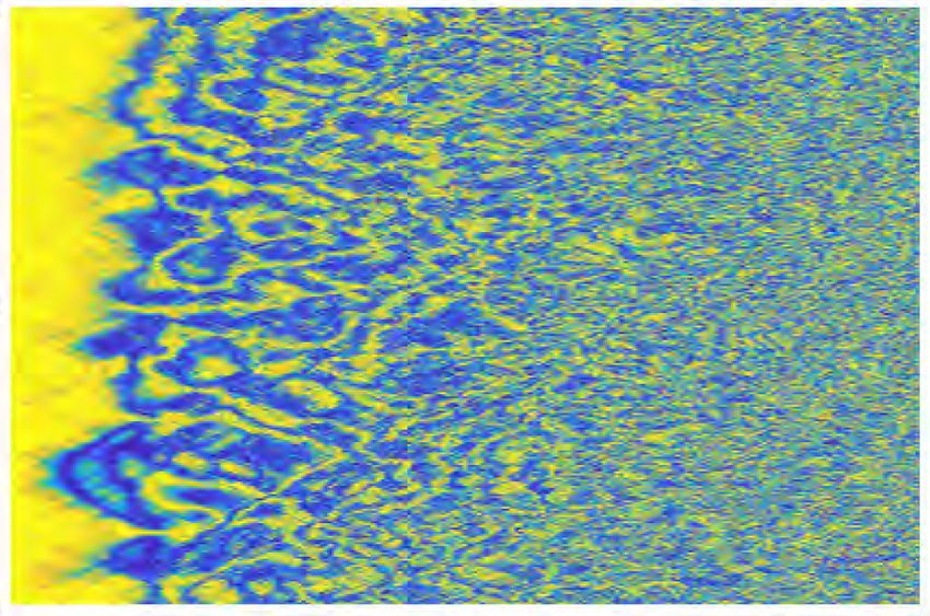
In addition, as shown in the single-trajectory example in below 0. We define a threshold value cosφa = 0.9 as the
Fig. 4, increasing the reduced temperature τ of the system initiation of the false vacuum tunneling event.
enhances the interactions between the false vacua and the Recalling that the TW method provides quantum esti-
true vacua on long time scales. In the example of the low- mation from a set of stochastic trajectories, to investigate
temperature dynamics shown in Fig. 3, domain-wall and thermal effects on the tunneling rate at finite-temperature
oscillon formation is minimized and the bubbles are well conditions, we repeat the single trajectory simulation and
defined. This clear structure of the true vacuum is disturbed determine the probability of bubble creation [cosφa ≤
when the BEC is strongly thermalized as shown in Fig. 4. 0.9] over time, P( t).
As can be seen in Fig. 4, no stable domain walls or We then obtain the survival probability of the false
periodic oscillons are formed as the temperature increases, t
vacuum F given that F = 1 − 0 P( t )d
t . The tunneling
and no true vacuum bubbles survive on long time scales.
rate for long time scales is calculated from a linear
As quantum tunneling is enhanced at higher temperatures,
fit in log scale given that F = exp(− t) [94]. We per-
more bubbles are formed in the true vacua, but most of
form simulations over a range of coupling strengths ν and
them are short lived. Tunneling is accelerated at high
reduced temperatures τ . Results are presented in Figs. 6,
temperatures, which leads to strong fluctuations between
7, and 8. Previous work showed that larger couplings ν
the true vacua and the false vacua, and many relatively
extend the tunneling time [15,16], which confirmed an
unstable domain walls.
expected slowing down of quantum tunneling with dis-
To quantify tunneling events, we can examine the aver-
sipation [95]. To illustrate thermal effects, we compare
age cosine of the relative phase of the coupled fields along
the Bogoliubov thermal-state results with the coherent-
state results, in which thermal noise is neglected. Although
the coherent initial state is not a true Bogoliubov ground
state, it has very similar behavior to the low-temperature
ground state. In the Wigner representation, the coherent
FIG. 5. Time evolution of the corresponding average relative
FIG. 4. Single-trajectory 1D false vacuum simulation for the phase cosφa shown in Fig. 3 (solid line) and Fig. 4 (dash line),
time evolution of pz at τ = 3 × 10⁻⁴ , all other parameters are as the horizontal dash-dot line cosφa = 0.9 indicates the threshold
in Fig. 3. of the appearance of a true vacuum bubble.
010350-13You can also read