Fear, Lockdown, and Diversion: Comparing Drivers of Pandemic Economic Decline 2020 - Austan Goolsbee and Chad Syverson - University of Chicago
←
→
Page content transcription
If your browser does not render page correctly, please read the page content below

WORKING PAPER · NO. 2020-80

Fear, Lockdown, and Diversion: Comparing
Drivers of Pandemic Economic Decline 2020
Austan Goolsbee and Chad Syverson
JUNE 2020

                                     5757 S. University Ave.
                                         Chicago, IL 60637
                                        Main: 773.702.5599
                                          bfi.uchicago.edu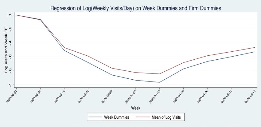
Fear, Lockdown, and Diversion:
    Comparing Drivers of Pandemic Economic Decline 2020

                                          Austan Goolsbee

                                           Chad Syverson *

                                        Version: June 17, 2020
                                             Preliminary

                                              Abstract

The collapse of economic activity in 2020 from COVID-19 has been immense. An important
question is how much of that collapse resulted from government-imposed restrictions on activity
versus people voluntarily choosing to stay home to avoid infection. This paper examines the drivers
of the economic slowdown using cellular phone records data on customer visits to more than 2.25
million individual businesses across 110 different industries. Comparing consumer behavior over the
crisis within the same commuting zones but across state and county boundaries with different policy
regimes suggests that legal shutdown orders account for only a modest share of the massive changes
to consumer behavior (and that tracking county-level policy conditions is significantly more accurate
than using state-level policies alone). While overall consumer traffic fell by 60 percentage points,
legal restrictions explain only 7 percentage points of this. Individual choices were far more
important and seem tied to fears of infection. Traffic started dropping before the legal orders were
in place; was highly influenced by the number of COVID deaths reported in the county; and showed
a clear shift by consumers away from busier, more crowded stores toward smaller, less busy stores in
the same industry. States that repealed their shutdown orders saw symmetric, modest recoveries in
activity, further supporting the small estimated effect of policy. Although the shutdown orders had
little aggregate impact, they did have a significant effect in reallocating consumer activity away from
“nonessential” to “essential” businesses and from restaurants and bars toward groceries and other
food sellers.

*
 Goolsbee: University of Chicago Booth School of Business and NBER,
austan.goolsbee@chicagobooth.edu. Syverson: University of Chicago and NBER,
chad.syverson@chicagobooth.edu. We would like to thank seminar participants at the University of
Chicago for their comments and SafeGraph, Inc. for making their data available for academic
COVID research. We thank Roxanne Nesbitt and, especially, Nicole Bei Luo for superb research
assistance and the Initiative on Global Markets at the University of Chicago for financial assistance.
The spread of the SARS-CoV-2 virus and its associated COVID-19 disease has had
unprecedented effects on economic activity around the world. In an effort to limit the spread of the
disease, many governments adopted stay-at-home/shelter-in-place orders. That ignited a debate over
“re-opening” and whether the health benefits from their slowing of the virus outweighs the
economic damage they did.
It is not clear, however, that the economic decline actually came from the lockdown orders.
By many accounts, anxious individuals engaged in physical distancing on their own accord.
Understanding the size of that effect is critical policy question. If fear rather than policy drives the
economics, the economic stimulus from repealing the orders may be considerably smaller than some
might predict.
In this paper, we estimate the causal effect of government policy on the economy during the
initial spread of COVID-19 in the U.S. using data on foot traffic at 2.25 million individual
businesses. Our empirical strategy separates the effects of voluntary distancing from that of policy
orders by comparing differences in foot traffic across businesses within commuting zones that span
jurisdictions facing differing legal restrictions. This leverages two related types of variation:
businesses in border-spanning commuting zones where jurisdictions impose of shelter-in-place
orders at different times (e.g., northern Illinois when Illinois placed a sheltering order on March 20th
while Wisconsin waited until the following week), and businesses in commuting zones where a
jurisdiction never imposed an order (e.g., the Quad Cities area, where the Illinois towns of Moline
and Rock Island faced stay-at-home orders but bordering Davenport and Bettendorf, Iowa did not).
We collect data on the shutdown policy conditions at the county level, rather than relying on state-
level laws as in most of the existing literature, because many of the hardest hit counties in the
country imposed shutdown orders earlier than their states did.
1The results indicate that legal shutdown orders account for a modest share of the massive
overall changes in consumer behavior. Total foot traffic fell by more than 60 percentage points, but
legal restrictions explain only around 7 percentage points of that. In other words, comparing two
similar establishments within a commuting zone but on opposite sides of a shelter-in-place (S-I-P)
order, both saw enormous drops in customer activity. The one on the S-I-P side saw a drop that was
only about one-tenth larger. The vast majority of the decline was due to consumers choosing of their
own volition to avoid commercial activity.
We find evidence tying this voluntary decline in commercial activity to fear of infection. The
drop in consumer visits is strongly correlated with the number of local COVID deaths. Further,
within an industry, drops in visits are disproportionately larger in establishments that were
busier/larger before COVID. This is consistent with greater avoidance of and substitution away
from establishments with higher potential transmission contacts.
Interestingly, and further supporting the modest size of the estimated S-I-P effects, when
some states and counties repealed their shutdown orders toward the end of our sample, the recovery
in economic activity due to the repeal was equal in size to the decline at imposition. Thus the
recovery is limited not so much by policy per se as the reluctance of individuals to engage in
economic activity that requires interacting with others.
Although the shutdown orders had a small aggregate impact, they had significant reallocation
effect by driving consumer activity from “nonessential” to “essential” businesses and from
restaurants and bars toward groceries and other food sellers.
There is a rapidly burgeoning empirical economics literature examining many aspects of the
COVID-19 pandemic. Our study is tied most closely to two areas of this literature. One involves
studies using cellular phone data to track how fear of the virus or lockdown orders have affected
personal mobility and interactions. Examples include Alexander and Karger (2020), Alfaro et al.
2(2020), Barrios et al. (2020), Chen et al. (2020), Cicala et al. (2020), Couture et al. (2020), Dave et al.
(2020a), Fang et al. (2020), Gupta et al. (2020), and Nguyen et al. (2020). Goldfarb and Tucker
(2020) tie personal mobility to retail activity by evaluating which retail industries have the most social
interaction. Maloney and Taskin (2020) demonstrate connections between mobility and commercial
activity in U.S. restaurants and Swedish movie theaters.
The second area of related work includes studies that focus directly on the economic impact
of lockdown policy, though with different data. Kahn et al. (2020) use job postings data to show that
the labor market deteriorated substantially but did so across the board, rather than more in states
with shutdown orders. Rojas et al. (2020) investigate UI claims and similarly find shifts across the
board. Bartik et al. (2020a, 20020b) study the impact of COVID on small businesses using survey
data and employment/hours using the HOMEBASE data set, documenting a significant
employment decline. Aum et al. (2020) look at the labor market effects of COVID in Korea (which
did not have large government imposed lockdowns) by comparing regions with larger COVID
outbreaks to ones with smaller and find employment collapses even without policy. Coibon et al.
(2020) do the same with survey data in the Nielsen panel so they can track aggregate spending and
find that lockdowns greatly reduce spending (though their measure of lockdown is a subjective
survey questions rather than an actual measure of policy). Gupta et al. (2020) look at CPS data and
argue that 60% of the decrease in employment came from state social distancing policy, though they
are unable to rule out the possibility that the employment drop began before the policies were in
place.
Our paper differs from these studies in that we combine detailed phone record location data
at the level of the business (rather than the individual) with more comprehensive data on legal
restrictions than what existed in previous work. This allows us to investigate not just patterns in
aggregate activity but substitution patterns across businesses as well. On the policy side, most studies
3use state level information on S-I-P orders and legal restrictions aggregated by sites like the New
York Times. In reality, however, a large number of counties and cities imposed lockdown orders
separately from their states and before the state acted. We demonstrate below that especially in
situations involving cross-border comparisons, the local policy data are important.
1. Data
Our data come from the SafeGraph panel of mobile phone usage (see SafeGraph, 2020 or
Squire, 2020, for more details). SafeGraph collects information on almost 45 million cellular phone
users—about 10% of devices in the U.S—and compiles the number of visits to millions of different
“points of interest” in the U.S. as specified by address. We will use this business level information.
In our sample, SafeGraph reported visit numbers excluding employees of the business. We focus on
business locations in industries where consumer visits are a plausible measure of economic activity
(not, for example, manufacturing facilities) and we drop non-profits and other non-commercial
enterprises. There are some complications and measurement errors that arise for businesses that are
co-located in a space like a Starbucks inside an subway station, say, so that the phone data might
record a large number of visits to the location but in reality, most of those were not to the business
in question. Our sample includes more than 2.25 million business locations and includes weekly
customer visitation data from March 1 to May 16 and monthly visitation data before that.
Implicitly we assume that the number of visits corresponds to the amount of economic
activity. If people shop half as frequently but spend twice as much each time they go out, we would
not observe that behavior. The timing of the aggregate drop in consumer visits, though, matches
well the broader economic declines. To combine industries into one regression and measure
aggregate effects, we weight businesses in our regressions by their average number of consumer
visits in January, before COVID. The results are largely identical if we weight by the product of
4January visits and the industry average revenue per visit (computed using supplemental industry
revenue data from the Census Bureau).
For policy measures, most of the literature has used state-level shutdown orders. However,
many lower levels of government imposed shutdown orders prior to their parent states acting. We
collected more detailed policy data that includes county-level orders and use that here. We describe
these data in Goolsbee et al. (2020) and will make it publicly available.
2. The Problem of Confounding Lockdown with Fear
Figure 1 shows the precipitous drop and partial recovery in visits to businesses in the
SafeGraph data over March, April, and early May. It shows two series, each measured using
establishments’ logged average visits per day across the week. The red line shows the raw data. The
blue line plots the values of the week fixed effects in a regression of logged visits on establishment
and week fixed effects. This latter series reflects average patterns over time controlling for any
changes in the composition of establishments in the sample. We normalize both series to a value of
zero in the first week of March for comparison purposes.
Both series show similar patterns. From the start of March to the trough in the week of
April 12th, the aggregate number of logged visits fell by around 0.9, a 60% decline. The suddenness
of this drop is similar to that in aggregate economic measures like the Weekly Economic Indicators
of Lewis et al. (2020) or the UI claims data. In the Appendix Table, we break down the start-to-
trough drop in visits for the 110 6-digit NAICS industries in our sample. It shows mostly expected
patterns in terms of severity of the downturn. Businesses in almost all industries saw large declines
in foot traffic, but they range from a 99% decline in the hardest hit industry, Theaters and Dinner
Theaters, to slight increase at Outdoor Power Equipment Stores at the other extreme.
5The question of how much of this collapse came from government regulations is not
immediately obvious in the figure. A simple time series correlation would suggest the two are
related, but if the spread of the virus both made people afraid to go out and induced states and
counties to impose lockdowns, the correlation could be spurious. Indeed, most jurisdictions did not
impose legal shutdown orders until late March or early April, but Figure 1 shows a considerable
collapse of commerce before most shutdown orders were in place.
The basic problem of with estimating the impact of policy becomes clear in Table 1. Here
we again combine all businesses together into a single regression, weighting each by their visits in
January. The dependent variable is the establishment’s log average number of visits in the week. The
key explanatory variable is an indicator for the existence of a shelter-in-place (S-I-P) order for the
establishment’s county in that week. The regression also includes establishment fixed effects. We
cluster the standard errors at the county level.
This “naïve” regression suggests a massive effect of S-I-P orders on economic activity. The
coefficient in column (1) indicates S-I-P orders correspond to a more than 70 log point decline in
consumer visits.
In column (2) we include both our county-level policy measure as well as an indicator for the
applicable state-level policy. The results indicate that the locally detailed measure explains far more
of the change in economic activity than the state-level measure, supporting our more geographically
detailed metrics.
Column (3) adds to the regression the cumulative number of COVID deaths in the county.
Because the death count distribution is highly skewed while still having many county-weeks with
zero cases, we use the logarithmic-like inverse hyperbolic sine transformation (see Burbridge, Magee
and Robb, 1988). As is apparent in the table, local deaths are strongly related to the size of the
reduction in consumer visits. Further, controlling for deaths both reduces the estimated impact of
6county S-I-P policy by 25%. Column (3) also thoroughly documents the importance of the county
level data instead of the state. The state-level policy coefficient is economically small, statistically
insignificant and of the wrong sign. We will use only the more detailed measure for the remaining
results.
Finally, in column (4), we add commuting-zone-by-week fixed effects. These fixed effects
control for any unobserved factors, like consumers’ average current fears of infection, that operate
across the geographic area in that week. It also means that the estimated effect of S-I-P orders in this
specification comes from comparing differences in consumer behavior within commuting zones but
across counties with different policies. Here, the estimated impact of shutdown orders falls by an
order of magnitude relative to that column (1), to a bit over 7%.
The comparison of the coefficient on the S-I-P order indicator in column (4) to those in the
table’s other columns is important. It shows the correlation between the decline in economic activity
and S-I-P policies arose mostly because the COVID crisis jointly drove both, not because S-I-Ps had
a large causal effect on activity. People greatly reduced their activity regardless of the existence of S-
I-P orders. The orders per se cut activity further in areas subject to them, but by only a modest
amount, around one-tenth of the total response.
The results in column (4) also demonstrate that even as the estimated impact of lockdown
policy is modest, local COVID deaths still significantly drive down consumer visits. The spread of
the disease itself is strongly correlated with declines in economic activity. Because the regression
includes commuting zone-week fixed effects, this indicates that even within commuting zones, more
local deaths reduce local economic activity. Interestingly, though, applying this within commuting-
zone coefficient at face value as an aggregate impact and multiplying by the overall increase in deaths
over our entire sample, the rise in COVID deaths would correspond to a decrease in economic
activity of around 30% or half the total decline observed in the data.
73. Robust Identification: The Modest Impact of Lockdowns Estimated Multiple Ways
Because there are two types of variation in the data—businesses in places where the
lockdowns occurred earlier on one side of a border than the other, and businesses in places where
one side of the border is in one of the eight states that never had a general lockdown—we can test
whether the estimated impact of lockdown orders is consistent across these sources of variation.
The results are in Table 2. Column (1) shows the estimated impact of lockdowns in the subsample
of only commuting zones that share a border with a jurisdiction that never had lockdown. Column
(2) looks only at businesses in the other commuting zones, where identification comes strictly from
timing differences in states’ and counties’ impositions of policies. The estimated impact is almost
identical in the two subsamples.
Then, in column (3), we look at potential asymmetries in S-I-P effects depending on whether
they are being imposed or repealed. By the end of our sample, some states and counties had repealed
their sheltering orders or let them expire, hoping this would restart economic growth. Our results
above, however, suggest that repealing the S-I-P orders should not matter much as long if people
still fear the spread of the virus. We examine this in more detail by allowing S-I-P repeals to have a
different coefficient than S-I-P impositions. Specifically, our repeal variable equals one when a
jurisdiction repeals its sheltering order, so the total effect of a repeal equals the negative of the S-I-P
order coefficient (i.e., as it turns from 1 to 0) plus the repeal coefficient. As seen in the table, the
repeal coefficient is small, negative, and not significantly different from zero. Thus the effect of
repealing a S-I-P order is statistically the mirror image of imposing one, and certainly no larger. The
point estimates imply economic activity fell 8% when governments instituted the orders and rose
5% when they repealed them.
8Repealing lockdowns may not a particularly powerful tool for restarting growth. If people
are otherwise concerned about potential infection, lifting legal restrictions on their activity has
limited effect. Moreover, such a policy would have to be balanced against the fact that S-I-P orders
may slow the spread of the disease—see, e.g., Baker et al. (2020), Chen et al. (2020), Dave et al.
(2020b, 2020c), or Friedson et al. (2020). If repealing lockdowns leads to a fast enough increase in
COVID infections and deaths and a concomitant withdrawal of consumers from the market place,
they might ultimately end up harming business activity.
4. Shifting: Time and Geography
In Table 3 we look for evidence of shifting/gaming of S-I-P orders. High frequency data
such as ours can give a misleading picture of policy impacts if, in the week prior to the policy being
put into place, people rush to engage in economic activity that would have otherwise waited until
later. Comparing before-and-after activity levels will overstate the effect of the policy because of this
intertemporal substitution. Similarly, the estimated impact of lockdowns will overstate their true
effect if consumers shift their commercial activity across borders. If customers in, say, Memphis,
Tennessee simply drove to Arkansas (where there was no statewide S-I-P order) to get their hair cut
when Memphis was under a sheltering order, it will look like the order causes a drop in activity even
though overall commercial activity did not change.
We investigate intertemporal shifting in column (1) of Table 3. Here, we include one-week
lags and leads of the policy. There is no evidence of anticipatory increases in consumer activity in the
week before S-I-P enactment and there is evidence that policy effects exhibit persistence once
imposed.
In column (2) we measure geographic shifting using as our dependent variable SafeGraph
data on the average distance traveled to a business among its customers that week. If the sort of
9cross-border shifting of activity from S-I-P jurisdictions to non-S-I-P jurisdictions is occurring, we
should see the average distance traveled rise substantially when S-I-P orders go into effect. We find
no such pattern; the point estimate is small, statistically insignificant, and negative.
These two pieces of evidence indicate that the effects of S-I-P orders, such as they are, do
not seem to induce a lot of intertemporal or spatial shifting of economic activity. Further, it is worth
noting that to the extent that any such shifting does occur, this will result in our estimates
overstating the true economic effect of S-I-P policies, meaning that even their modest size is an
upper bound.
5. Fear and the Choice of Big Versus Small Business
In this section we document differential patterns in the slowdown across stores of different
sizes. People afraid of infection may avoid larger, busier stores in favor of smaller options with fewer
visitors. Our results indicate this is what happened, further suggesting fear of the virus is an
overriding determinant of people’s decisions to engage in economic activity.
We divide the businesses up within their state-by-industry cell based on their size/traffic
before COVID arrived (we use the total number of consumer visits to the location in January). We
then classify each establishment into one of three size groupings within its state-industry: smallest
20%, middle 60% and largest 20%. For instance, we rank all Grocery Stores in Wisconsin by their
traffic in January; the busiest 20% are in the top size/traffic category, and so on.
We first regress the number of weekly visits to a business on establishment fixed effects and
separate week fixed effects for each of the three business size quantiles. We plot these week-by-
quantile fixed effects in Figure 2. Activity falls for all businesses, but falls dramatically more for
large, high-traffic businesses than for smaller, less busy ones. At the trough, traffic is down over
70% at the largest establishments, but only about 45% at the smallest ones. Consumers are
10substituting away relatively more from industry businesses that pose a greater probability of contact
with others. 1
In column (1) of Table 4, we measure this differential size response statistically by looking at
the change in establishments’ log daily visits from January 2020 to the trough week of April 12 as a
function of the establishment’s size quantile within its industry-state. Relative to their industry
cohorts in the middle 60% of the size distribution, small businesses had considerably more traffic at
the trough (they had lost traffic on average, but considerably less than the larger businesses did). The
difference is about 50 log points, or over 60%. Conversely, the largest 20% of establishments saw a
larger decline in traffic, about 30% more, than did the middle quantile.
Column (2) interacts the number of local COVID deaths with the business size categories.
Localities where the disease is more prevalent see a more pronounced relative shift away from large
businesses and toward small ones, consistent with fear of infection driving consumer behavior.
Column (3) shows that S-I-P policies themselves also lead to larger shifts away from the biggest
establishments.
6. Lockdowns and Business Diversion
The evidence points to a modest impact of shutdown orders on aggregate economic activity
However, the orders can still have a significant impact on the types of businesses that consumer visit.
We see that in the size results above, but potentially even more extreme responses might be induced
when shutdown orders target specific types of businesses. In this section, we use the information
from Goolsbee et al. (2020) on government restrictions on activity at restaurants and bars and,
1 We repeated this exercise using data from the same time period in 2019 to investigate if this might be just a seasonal
effect. It did not show the same pattern. We also examined whether survivor bias might make it only seem that small
businesses do better, because small firms that die do not get counted. Imputing zero visits for missing firms and using
the inverse hyperbolic sine transformation for visits yielded the same basic patterns as in Figure 2, however.
11separately, restrictions of ‘non-essential’ businesses (and which industries the policies classified as
‘non-essential’). 2 The results show substantial reallocations across types of businesses.
Table 5 interacts these policy measures with indicators for the type of business. The results
indicate that, indeed, even though general S-I-P orders reduced consumer visits by only around 5%,
orders limiting the activities of defined “non-essential” business reduce visits to those establishments
by a massive amount while at the same time increasing activity by roughly the same magnitude at
“essential” business. Similarly, restaurant and bar restrictions reduced consumer visits to bars and
restaurants by almost 30%, but they increased visits to non-restaurant food and beverage stores by
27%, and visits to all other businesses slightly.
7. Conclusion
The COVID-19 crisis led to an enormous reduction in economic activity. We estimate that
the vast majority of this drop is due to individuals’ voluntary decisions to disengage from commerce
rather than government-imposed restrictions on activity. Several patterns in the data are consistent
with these decisions reflecting people’s concerns that commerce may expose them to the disease.
We do not find evidence of large temporal or spatial shifting in response to shelter-in-place policies.
While their aggregate effect is modest, restrictions on activity that target particular types of
businesses do induce large reallocations of activity away from “disallowed” businesses and toward
“allowed” ones.
Our results come with caveats. While we do have data on 110 industry groupings—mostly
retail, personal services, restaurants and bars, and recreational industries—where customer foot
traffic is a reasonable proxy for economic activity, we do not measure policies’ effects on activity in
2We were not able to find essential business definitions systematically at the county level, so we are relying on the state
definitions even in the counties that acted before their states.
12other sectors. Moreover, we cannot measure the dollar volume of transactions per visit, though if we
weight by the average of such volume in the pre-COVID period, our results remain.
13References
Alexander, Diane and Ezra Karger. 2020. “Do Stay-at-Home Orders Cause People to Stay at Home?
Effects of Stay-at-Home Orders on Consumer Behavior.” FRB of Chicago Working Paper
WP 2020-12.
Alfaro, Laura, Ester Faia, Nora Lamersdorf, and Farzad Saidi. 2020. “Social Interactions in
Pandemics: Fear, Altruism, and Reciprocity.” NBER Working Paper 27134.
Aum, Sangmin, Sang Yoon (Tim) Lee, and Yongseok Shin. 2020. “COVID-19 Doesn’t Need
Lockdowns to Destroy Jobs: The Effect of Local Outbreaks in Korea.” NBER Working
Paper 27264.
Barrios, John M., Efraim Benmelech, Yael V. Hochberg, Paola Sapienza, and Luigi Zingales. 2020.
“Civic Capital and Social Distancing during the Covid-19 Pandemic.” NBER Working Paper
27320.
Bartik, Alexander W., Marianne Bertrand, Zoë B. Cullen, Edward L. Glaeser, Michael Luca, and
Christopher T. Stanton. 2020. “How Are Small Businesses Adjusting to COVID-19? Early
Evidence from a Survey.” NBER Working Paper 26989.
Benzell, Seth G., Avinash Collis, and Christos Nicolaides. 2020. “Rationing Social Contact during
the COVID-19 Pandemic: Transmission Risk and Social Benefits of US Locations.”
Working Paper.
Burbidge, John, Lonnie Magee, and A. Leslie Robb. 1988. “Alternative Transformations to Handle
Extreme Values of the Dependent Variable.” Journal of the American Statistical Association,
83(401): 123-127.
Chen, Keith, Yilin Zhuo, Malena de la Fuente, Ryne Rohla, and Elisa F. Long. 2020. “Causal
Estimation of Stay-at-Home Orders on SARS-CoV-2 Transmission.” UCLA Anderson
School Working Paper, May 15, 2020.
Cicala, Steve, Stephen P. Holland, Erin T. Mansur, Nicholas Z. Muller, and Andrew J. Yates. 2020.
“Expected Health Effects of Reduced Air Pollution from COVID-19 Social Distancing.”
Working Paper.
Coibon, Olivier, Yuriy Gorodnichenko, and Michael Weber. 2020. “The Cost of the Covid-19 Crisis:
Lockdowns, Macroeconomic Expectations, and Consumer Spending.” NBER Working
Paper 27141.
Couture, Victor, Jonathan Dingel, Allison Green, and Jessie Handbury. 2020. “Quantifying Social
Interactions Using Smartphone Data.” Working Paper.
Dave, Dhaval M., Andrew I. Friedson, Kyutaro Matsuzawa, Drew McNichols, and Joseph J. Sabia,
“Did the Wisconsin Supreme Court Restart a COVID-19 Epidemic? Evidence from a
Natural Experi ment,” NBER Working Paper No. 27322, June 2020.
14Dave, Dhaval M., Andrew I. Friedson, Kyutaro Matsuzawa, and Joseph J. Sabia. 2020. “When Do
Shelter-in-Place Orders Fight COVID-19 Best? Policy Heterogeneity across States and
Adoption Time.” NBER Working Paper 27091.
Dave, Dhaval M., Andrew I. Friedson, Kyutaro Matsuzawa, Joseph J. Sabia, and Samuel Safford.
2020. “Were Urban Cowboys Enough to Control COVID-19? Local Shelter-in-Place Orders
and Coronavirus Case Growth.” NBER Working Paper 27229.
Fang, Hanming, Long Wang, and Yang Yang. 2020. “Human Mobility Restrictions and the Spread
of the Novel Coronavirus (2019-nCoV) in China.” NBER Working Paper 26906.
Friedson, Andrew I., Drew McNichols, Joseph J. Sabia, and Dhaval Dave. 2020. “Did California’s
Shelter-in-Place Order Work? Early Coronavirus-Related Public Health Effects.” NBER
Working Paper 26992.
Goldfarb, Avi, and Catherine Tucker. 2020. “Which Retail Outlets Generate the Most Physical
Interactions?” NBER Working Paper 27042.
Goolsbee, Austan, Nicole Bei Luo, Roxanne Nesbitt, and Chad Syverson. 2020. “COVID-19
Lockdown Policies at the State and Local Level.” Technical Note.
Gupta, Sumedha, Laura Montenovo, Thuy Nguyen, Felipe Lozano Rojas, Ian M. Schmutte, Kosali I.
Simon, Bruce A. Weinberg, and Coady Wing. 2020. “Effects of Social Distancing Policy on
Labor Market Outcomes.” NBER Working Paper 27280.
Gupta, Sumedha, Thuy D. Nguyen, Felipe Lozano Rojas, Shyam Raman, Byungkyu Lee, Ana Bento,
Kosali I. Simon, and Coady Wing. 2020. “Tracking Public and Private Responses to the
COVID-19 Epidemic: Evidence from State and Local Government Actions.” NBER
Working Paper 27027.
Lewis, Daniel, Karel Mertens, and James H. Stock. 2020. “U.S. Economic Activity during the Early
Weeks of the SARS-Cov-2 Outbreak.” NBER Working Paper 26954.
Maloney, William and Temel Taskin. 2020. “Social Distancing and Economic Activity during
COVID-19: A Global View.” COVID Economics, Issue 13.
Nguyen, Thuy D., Sumedha Gupta, Martin Andersen, Ana Bento, Kosali I. Simon, and Coady Wing.
2020. “Impacts of State Reopening Policy on Human Mobility.” NBER Working Paper
27235.
Rojas, Felipe Lozano, Xuan Jiang, Laura Montenovo, Kosali I. Simon, Bruce A. Weinberg, and
Coady Wing. 2020. “Is the Cure Worse than the Problem Itself? Immediate Labor Market
Effects of COVID-19 Case Rates and School Closures in the U.S.” NBER Working Paper
27127.
SafeGraph, 2020. Documentation Tab. https://docs.safegraph.com/docs
15Squire, Ryan Fox. 2019. “What About Bias in the SafeGraph Dataset?”
https://www.safegraph.com/blog/what-about-bias-in-the-safegraph-dataset, accessed May
28, 2020.
16TABLE 1: STANDARD POLICY ESTIMATE: LN (VISITS/DAY)
(1) (2) (3) (4)
S-I-P Order -0.714 -0.599 -0.545 -0.076
(0.015) (0.016) (0.016) (0.011)
State S-I-P -0.124 0.022
(0.014) (0.017)
ln(County deaths) -0.102 -0.030
[asinh transf] (0.006) (0.005)
N 23,865,724 23,865,724 23,865,724 23,865,721
R2 0.853 0.853 0.858 0.880
FEs Store Store Store Store
C-Zone x Week
Weights: Visits in Jan Visits in Jan Visits in Jan Visits in Jan
Cluster SE: County County County County
Notes: The dependent variable is log number of average consumer visits per day to the store. S-I-P Order is
the measure of shelter-in-place at the county level or at the state level as described in the text. The measure of
County deaths is the log of an inverse hyperbolic sine transformation of the number of deaths in the county
to account for the many zeros. The standard errors are clustered at the county level.
17TABLE 2: BETTER IDENTIFIED POLICY ESTIMATE: LN (VISITS/DAY)
(1) (2) (3)
Border No Border Exit/Repeal
S-I-P Order -0.068 -0.080 -0.082
(0.014) (0.014) (0.011)
Repeal Order -0.030
(0.028)
ln(County deaths) -0.032 -0.042 -0.039
[asinh transf] (0.011) (0.006) (0.005)
N 6,391,240 17,474,481 23,865,721
R2 0.873 0.882 0.880
FEs Store Store Store
CZ x Week CZ x Week CZ x Week
Weights: Visits in Jan Visits in Jan Visits in Jan
Cluster SE: County County County
Notes: The dependent variable is log number of average consumer visits per day to the store. S-I-P Order is
the measure of shelter-in-place at the county level as described in the text. Repeal Order indicates locations
where they repeal or let their order expire. The measure of County deaths is the log of an inverse hyperbolic
sine transformation of the number of deaths in the county to account for the many zeros. The standard
errors are clustered at the county level.
18TABLE 3: SHIFTING
(1) (2)
Intertemporal Ln(Distance)
S-I-P Order (t+1) -0.008 (0.009)
S-I-P Order (t) -0.064 (0.010) -0.015 (0.013)
S-I-P Order (t-1) -0.054 (0.009)
ln(county deaths) -0.039 (0.005) -0.001 (0.005)
[asinh transf]
N 23,285,721 17,645,439
R2 0.880 0.780
FEs Store Store
CZ x Week CZ x Week
Weights: Visits in Jan Visits in Jan
Cluster SE: County County
Notes: The dependent variable is log number of average consumer visits per day to the store in (1) and the
log of average distance traveled to the store in (2). S-I-P Order is the measure of shelter-in-place at the county
level as described in the text and the time script indicates whether the measure is contemporaneous, lagged or
led one week. The measure of County deaths is the log of an inverse hyperbolic sine transformation of the
number of deaths in the county to account for the many zeros. The standard errors are clustered at the
county level.
19TABLE 4: SIZE OF BUSINESS: CHANGE LN(VISITS/DAY): JAN. TO APRIL 12
(1) (2) (3)
SIZE DEATHS POLICY
{S=1: Small 20%} 0.491 (0.004) 0.445 (0.011) 0.400 (0.021)
{L=1: Large 20%} -0.352 (0.004) -0.239 (0.019) -0.259 (0.022)
ln(county deaths) -0.070 (0.010) -0.088 (0.010)
ln(county deaths) x {S=1} 0.014 (0.005)
ln(county deaths) x {L=1} -0.032 (0.007)
S-I-P Order -0.039 (0.064)
S-I-P Order x {S=1} 0.084 (0.022)
S-I-P Order x {L=1} -0.094 (0.026)
N 2,106,343 2,106,343 2,106,343
R2 0.080 0.080 0.882
FEs CZ CZ CZ
Cluster SE: County County County
Notes: The dependent variable is the change in log number of average consumer visits per day to the store
from January to the week of April 12th. The {S=1} variable indicates a firm is in the smallest 20% of firms in
its state x industry measured as total visits in the month of January. The {L=1} variable indicates a firm in the
largest 20% of firms by the same measure. The measure of County deaths is the log of an inverse hyperbolic
sine transformation of the number of deaths in the county to account for the many zeros. The standard
errors are clustered at the county level.
20TABLE 5: BUSINESS DIVERSION
(1)
S-I-P Order -0.046 (0.017)
Restaurant Order x {Restaurant=1} -0.289 (0.008)
Restaurant Order x {Food=1} 0.275 (0.009)
Restaurant Order 0.054 (0.013)
Essential Biz Order x {Essential=1} 0.475 (0.012)
Essential Biz Order -0.382 (0.028)
Ln (cnty deaths) [asinh transform] -0.035 (0.005)
N 23,865,721
R2 0.885
FEs Store
CZ x Week
Cluster SE: County x Essential
Notes: The dependent variable is log number of average consumer visits per day to the store. S-I-P Order is
the measure of shelter-in-place at the county level as described in the text. The other variables define essential
and non-essential businesses, restaurants and bars, and non-restaurant food and beverage businesses as
described in the text. The measure of County deaths is the log of an inverse hyperbolic sine transformation of
the number of deaths in the county to account for the many zeros. The standard errors are clustered at the
county x essential business level.
21APPENDIX TABLE: CHANGE IN LN(VISITS/DAY): JAN. TO APRIL 12
Worst 15 industries Dln(v/day) Best 15 industries Dln(v/day)
711190 Other Perf. Arts -4.33 444210 Outdoor pwr eq stores +0.17
711110 Theaters -3.85 444220 Nurse/grdn/farm s. +0.03
713920 Skiing facilities -3.60 713910 Golf courses +0.01
712130 Botanic gardens, zoos -3.49 811411 Home &garden eq rpr -0.18
811219 Other elec eq rpr -3.16 541940 Veterinary services -0.57
711211 Sports teams -2.50 444130 Hardware store -0.60
512131 Motion picture thtrs -2.44 722320 Caterers -0.62
448150 Clothing acc. stores -2.35 447190 Gasoline stations -0.63
711219 Other spect sports -2.10 445110 Supermarkets -0.63
713950 Bowling centers -2.08 445120 Convenience stores -0.64
448320 Luggage stores -1.93 454310 Fuel dealers -0.66
722410 Drinking places (alc) -1.90 441222 Boat dealers -0.67
448140 Family clothing s. -1.87 441228 Motorcycle, atv dealers -0.67
812990 Other pers services -1.82 441310 Auto parts stores -0.69
713940 Fitness centers -1.75 446110 Pharmacies -0.72
Notes: This is the raw change in the log number of visits per day from January 2020 to the week of
April 12th by industry for the worst performing and best performing 6-digit NAICS codes in our
sample.
22FIGURE 1: AGGREGATE CONSUMER VISITS OVER TIME
FIGURE 2: CONSUMER VISITS OVER TIME BY STORE SIZE/TRAFFIC
23You can also read