Fire and Mechanical Forest Management Treatments Support Different Portions of the Bird Community in Fire-Suppressed Forests - MDPI
←
→
Page content transcription
If your browser does not render page correctly, please read the page content below
Article
Fire and Mechanical Forest Management Treatments Support
Different Portions of the Bird Community in
Fire-Suppressed Forests
Lance Jay Roberts * , Ryan Burnett                    and Alissa Fogg

                                          Point Blue Conservation Science, Petaluma, CA 94952, USA; rburnett@pointblue.org (R.B.);
                                          afogg@pointblue.org (A.F.)
                                          * Correspondence: ljroberts@pointblue.org

                                          Abstract: Silvicultural treatments, fire, and insect outbreaks are the primary disturbance events
                                          currently affecting forests in the Sierra Nevada Mountains of California, a region where plants
                                          and wildlife are highly adapted to a frequent-fire disturbance regime that has been suppressed for
                                          decades. Although the effects of both fire and silviculture on wildlife have been studied by many,
                                          there are few studies that directly compare their long-term effects on wildlife communities. We
                                          conducted avian point counts from 2010 to 2019 at 1987 in situ field survey locations across eight
                                          national forests and collected fire and silvicultural treatment data from 1987 to 2016, resulting in a
                                          20-year post-disturbance chronosequence. We evaluated two categories of fire severity in comparison
                                          to silvicultural management (largely pre-commercial and commercial thinning treatments) as well as
                                          undisturbed locations to model their influences on abundances of 71 breeding bird species. More
                                          species (48% of the community) reached peak abundance at moderate-high-severity-fire locations

                                   than at low-severity fire (8%), silvicultural management (16%), or undisturbed (13%) locations. Total
                                          community abundance was highest in undisturbed dense forests as well as in the first few years
Citation: Roberts, L.J.; Burnett, R.;
Fogg, A. Fire and Mechanical Forest
                                          after silvicultural management and lowest in the first few years after moderate-high-severity fire,
Management Treatments Support             then abundance in all types of disturbed habitats was similar by 10 years after disturbance. Even
Different Portions of the Bird            though the total community abundance was relatively low in moderate-high-severity-fire habitats,
Community in Fire-Suppressed              species diversity was the highest. Moderate-high-severity fire supported a unique portion of the
Forests. Forests 2021, 12, 150.           avian community, while low-severity fire and silvicultural management were relatively similar. We
https://doi.org/10.3390/                  conclude that a significant portion of the bird community in the Sierra Nevada region is dependent
f12020150                                 on moderate-high-severity fire and thus recommend that a prescribed and managed wildfire program
                                          that incorporates a variety of fire effects will best maintain biodiversity in this region.
Academic Editor: Brice B. Hanberry
Received: 31 December 2020
                                          Keywords: fire; forest management; fuel treatment; disturbance; birds; Sierra Nevada
Accepted: 22 January 2021
Published: 28 January 2021

Publisher’s Note: MDPI stays neutral
                                          1. Introduction
with regard to jurisdictional claims in
published maps and institutional affil-        The management of multi-use forests is a vital component of global biodiversity
iations.                                  conservation, long-term carbon storage, economic well-being, recreation, and ecosystem
                                          sustainability [1,2]. Forest ecosystems worldwide face numerous current and emerging
                                          threats [3,4]. Among these threats is alteration of natural disturbance regimes, which may
                                          reduce forest resilience to climate change and other emerging threats [5–8].
Copyright: © 2021 by the authors.
                                               Fire is the fundamental disturbance process in seasonally dry conifer forests of western
Licensee MDPI, Basel, Switzerland.
                                          North America [9,10]. The suppression of fire over the past century has had profound effects
This article is an open access article
                                          by altering the vegetative composition and structure across the region [11,12]. Though the
distributed under the terms and           frequency of fires has increased sharply since the mid-1980s [13], and is likely to remain
conditions of the Creative Commons        higher than during the latter half of the 20th century [14], average fire return intervals
Attribution (CC BY) license (https://     are still far longer today than pre-suppression and the area burned is far smaller [15–18].
creativecommons.org/licenses/by/          In the Sierra Nevada Mountains of California (Figure 1), the reduced presence of fire
4.0/).                                    combined with past silvicultural activities (e.g., 20th-century tree harvest and reforestation)

Forests 2021, 12, 150. https://doi.org/10.3390/f12020150                                                     https://www.mdpi.com/journal/forests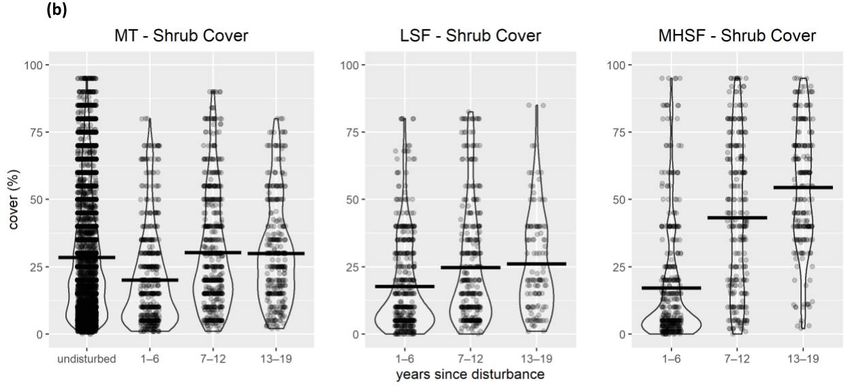
Forests 2021, 12, x FOR PEER REVIEW 2 of 24
Forests 2021, 12, 150 2 of 24
[15–18]. In the Sierra Nevada Mountains of California (Figure 1), the reduced presence of
fire combined with past silvicultural activities (e.g., 20th-century tree harvest and refor-
has led tohas
estation) a decrease in large in
led to a decrease trees,
largehigher densities
trees, higher of smaller-size
densities trees [19–21],
of smaller-size and
trees [19–21],
more homogeneous
and more forests
homogeneous with reduced
forests shade-intolerant
with reduced plant plant
shade-intolerant assemblages [22–26].
assemblages This
[22–26].
disturbance deficit
This disturbance has likely
deficit resulted
has likely in profound
resulted in profoundeffects onon
effects the
thewildlife
wildlifecommunity
community
composition
compositionandandstructure,
structure,e.g.,
e.g.,[27,28].
[27,28].
Figure1.1. Study
Figure Study area
area in
in the
the Sierra Nevada Mountains
Mountains of
of California,
California,USA.
USA.The
TheSierra
SierraNevada
NevadaCon-
Con-
servancy(SNC,
servancy (SNC, https://sierranevada.ca.gov/)
https://sierranevada.ca.gov/) boundary indicates
boundary thethe
indicates extent of the
extent study
of the region,
study region,
andthe
and theshaded
shadedarea
area indicates
indicates locations
locations within the ownership boundaries
boundaries of
of USDA
USDA Forest
ForestService
Service
nationalforest
national forestlands.
lands.
Natural disturbance
Natural disturbance regimes
regimes are arerecognized
recognizedas asfundamental
fundamentalto tothe
themaintenance
maintenanceof of
aviancommunities
avian communitiesininNorth NorthAmerica
America [29].
[29]. There
There is is a growing
a growing body body of evidence
of evidence support-
supporting
ingimportance
the the importance of burned
of burned landscapes
landscapes to to fire-prone
fire-prone forest
forest bird
bird communitiesininwestern
communities western
North America,
North America, e.g.,
e.g.,[27,30,31].
[27,30,31]. TheThe magnitude
magnitude of of vegetation
vegetation change change resulting
resultingfromfromall all
types
types ofof disturbances has has aaprimary
primaryrole roleininsetting
setting thethe post-disturbance
post-disturbance successional
successional tra-
trajectory
jectory and andhashas
beenbeen shown
shown to beto important
be important in fires
in fires as measured
as measured by severity
by severity [30,32].
[30,32]. Fire
Fire severity
severity is typically
is typically measured
measured as anasindex
an index of amount
of the the amount of change
of change in thein vegetation
the vegetationvisi-
visible to satellites,
ble to satellites, which which
is theis tallest
the tallest vegetation
vegetation layer layer in a [33].
in a stand standTypically,
[33]. Typically,
in forestedin
forested stands,
stands, when when
a fire a fire consumes
consumes canopy vegetation,
canopy vegetation, it will burn it willlowerburn lower vegetation
vegetation layers as
layers as well,
well, while while low-severity
low-severity fire oftenfire often consumes
consumes understory understory
and ground andvegetation
ground vegetation
but leaves
but leaves the overstory intact. Mechanical fuel reduction
the overstory intact. Mechanical fuel reduction treatments can differ in the treatments can differ of
amount in veg-
the
amount of vegetation
etation removed removedvertical
in different in different
strata,vertical
though strata,
in dry though
fire-prone in dry fire-prone
western western
forests, they
forests,
generallytheytarget
generally target vegetation
vegetation removal from removal fromlayers,
multiple multiple layers, including
including the canopy, the canopy,
subcan-
subcanopy, and understory
opy, and understory [34]. the
[34]. While While the negative
negative effects ofeffects
fires of
arefires
wellare well known,
known, there arethere
also
are also many benefits to ecosystems that have evolved with fire [35,36].
many benefits to ecosystems that have evolved with fire [35,36]. Increased habitat hetero- Increased habitat
heterogeneity promulgated
geneity promulgated by firebycan
firepromote
can promote higherhigher biodiversity
biodiversity [31]. [31]. Additionally,
Additionally, it is
it is clear
clear
that the early-seral forest habitat created by high-severity fire provides a habitat foraa
that the early-seral forest habitat created by high-severity fire provides a habitat for
number
numberof ofwildlife
wildlifespecies
species[37],
[37],with
withmany
manyassociated
associatedwith,with,and andin insome
somecasescasesdependent
dependent
on, particular combinations of severity and time since the
on, particular combinations of severity and time since the fire [27,28,38,39].fire [27,28,38,39].
While fire has been suppressed over the past century, mechanical timber harvest has
replaced fire as the primary disturbance in these forests. Mimicking natural disturbances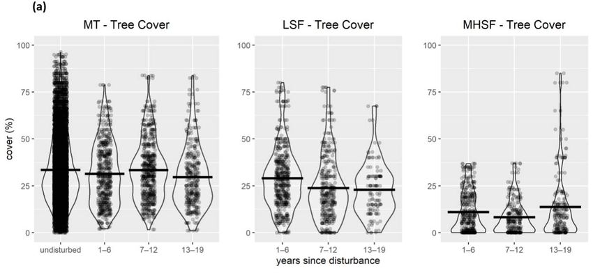
Forests 2021, 12, 150                                                                                                3 of 24

                        such as fire through forest silvicultural management has been advocated as a practical
                        alternative to conserve biodiversity in fire-adapted forests [40,41]. With the challenges of re-
                        introducing fire to its historic extent in western North American forests, forest management
                        policies have promoted emulation silviculture, a strategy that attempts to use mechanical
                        timber harvest to mimic the structural legacy of natural fire [42–45]. Within these forests,
                        effects of managing landscapes for reduced fuel loads has been shown to have relatively
                        small effects on the existing bird community composition [46–49]. However, the main
                        benefit of disturbance, in a disturbance starved system, may not be to maintain the status
                        quo but rather to provide a habitat for those species most closely tied to conditions created
                        by the natural disturbance regime [50].
                              Much of the management activity in Sierra Nevada forests today is targeted toward
                        reducing the severity of fires by reducing fuel loads to provide more opportunities for
                        future fire containment and suppression [51–53]. Fuels treatments generally aim to reduce
                        surface and ladder fuels, as well as overall stand density, targeting small- to medium-
                        size trees and understory vegetation for removal to promote slower rates of fire spread
                        and lower severity [54,55]. Following both fires and forest management, the vegetation
                        structure and composition can respond in a variety of ways, including increased herbaceous
                        and shrub cover, tree recruitment, and changes in ephemeral structural components such
                        as snags [56,57].
                              There are considerable efforts at state and federal levels to restore fire-prone, disturbance-
                        starved forests in California and across the U.S. Restoration of these forests is likely to
                        require employment of a broad range of tools, including mechanical treatments, prescribed
                        fire, and wildland fire [58–60]. As such, there is a corresponding need to understand how
                        wildlife species respond to these different potential restoration treatments [35]. There is
                        evidence that fire sets in motion successional processes that may or may not be similar to the
                        successional process following silvicultural activities [61,62], and may result in disparate
                        responses of wildlife [63,64]. A better understanding of the similarities and differences in
                        avian responses to fire and mechanical treatments can help guide a balanced approach to
                        forest management over space and time to maintain natural levels of biodiversity in these
                        natural disturbance-starved systems.
                              In this study, we evaluated the effects of fire and silvicultural disturbances on the avian
                        community in actively managed national forests of the Sierra Nevada over a 20-year post-
                        disturbance time period. We sought to understand how the most common disturbances
                        and a suite of other factors influence the abundances of avian species. We used data from an
                        extensive avian-monitoring program [65] to evaluate total bird abundance, diversity, and
                        the abundance of 71 individual species across the first two decades following mechanical
                        timber harvest, prescribed and low-severity fire, and moderate- and high-severity fire. We
                        also assessed the dissimilarity between avian assemblages within each of these categories to
                        assess the differences in the overall community composition among these land categories.

                        2. Materials and Methods
                        2.1. Study Location
                             Our study was performed within the Sierra Nevada and southern Cascade Mountains
                        in California, U.S. (Figure 1). We sampled birds within 8 national forest management units
                        that encompass nearly 3 million hectares, including Sequoia, Sierra, Stanislaus, Eldorado,
                        Tahoe, Plumas, and Lassen National Forests and the Lake Tahoe Basin Management Unit.
                        Our study area was defined as all upland forest and montane chaparral that is available
                        for management within the national forest boundaries [65]. No specific permits were
                        required to conduct this work, either by the land manager or by the wildlife agency, and
                        the coordinates of all study locations are available online [66]. This study did not involve
                        any threatened or endangered species.
                             The climate is Mediterranean, with the majority of precipitation occurring from
                        November to March and falling primarily as snow at the higher elevations and rain
                        elsewhere. Precipitation generally increases with elevation. The study area consists pre-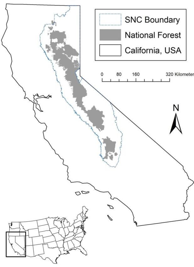
Forests 2021, 12, 150                                                                                            4 of 24

                        dominantly of Sierra mixed-conifer and true-fir cover types with smaller amounts of mon-
                        tane chaparral and hardwood-dominated habitat. Within the conifer forests, ponderosa
                        pine (Pinus ponderosa) is dominant at lower elevations; mixed-conifer forests comprising
                        ponderosa pine, white fir (Abies concolor), sugar pine (Pinus lambertiana), Douglas fir (Pseu-
                        dotsuga menzeisii), and incense cedar (Calocedrus decurrens) are dominant at intermediate
                        elevations and often intermixed with several hardwood species (e.g., Quercus spp.); and
                        white fir, red fir (Abies magnifica), Jeffrey pine (Pinus jeffreyi), and lodgepole pine (Pinus
                        contorta) are dominant at higher elevations.

                        2.2. Site Selection
                              Field data were assembled from a bioregional monitoring project designed to monitor
                        trends in upland forest birds inhabiting actively managed national forest lands. Survey
                        locations were selected using a generalized random tessellation stratified (GRTS) sampling
                        protocol [67,68]. The set of potential survey locations was built from a tessellation generated
                        in ArcGIS (ver. 9.2; Environmental Systems Research Institute, Redlands, CA, USA),
                        consisting of a grid of 1 km2 ; cells with a random origin covering the entire study area. To
                        more accurately represent the areas available to silvicultural management, we limited the
                        study area to locations within 1 km of accessible roads and slopes less than 35%. We overlaid
                        a vegetation layer of 35 different California Wildlife Habitat Relationship (CWHR) land
                        cover types (https://map.dfg.ca.gov/metadata/ds1327.html) and eliminated habitat types
                        such as grassland, sagebrush, riparian, foothill chaparral, oak woodland, subalpine, barren,
                        and juniper that were not subject to typical silvicultural treatments. Sample locations
                        ranged in elevation from 1003 to 2871 m and latitudes from 35.3906◦ to 41.2931◦ . At each
                        survey location, we established two transects in adjacent 1 km grid cells. Transects were
                        made up of four point count stations at 250 m in the cardinal directions from a fifth station
                        in the center. This resulted in a sample of 1987 stations on 398 transects distributed as 199
                        spatially balanced pairs.
                              We then assigned a history of fire and management at each point count station loca-
                        tion. To do this we overlaid the points on the Forest Service Activities Tracking System
                        (FACTS [69]) to identify the subsample of stations that had been mechanically treated, as
                        well as a fire severity assessment map [33,70], to identify the subsample of stations that
                        have burned. We identified all stations within GIS polygons labeled with FACTS activity
                        codes that indicated that a silvicultural treatment had occurred through mechanical means
                        (records were available from 1995 through 2016). The FACTS polygons that we included
                        in our sample were labeled with activity codes indicating that thinning treatments were
                        conducted using mechanical machinery (e.g., tractors, skidders, harvesters, feller-bunchers,
                        yarders, skylines, or helicopters). These activities included pre-commercial thin or tree
                        release and weed (49% of treatments), commercial thinning (39%), insect and disease con-
                        trol (11%), clearcuts (1%), and wildlife habitat improvements (76 cm DBH) and maintenance of canopy cover of over 40% [71].
                        Typical mechanical treatments at our study sites during the study period (since 1995 when
                        the FACTS database records began) consisted of several fuel reduction or stand improve-
                        ment treatments, often, but not always, including removal of merchantable overstory trees.
                        Fuel reductions and pre-commercial thinning treatments were focused on removing ladder
                        fuels (shrubs, small trees, some overstory), while leaving the largest trees (e.g., shaded fuel
                        break). The removal of these understory fuels left behind stands that were more likely to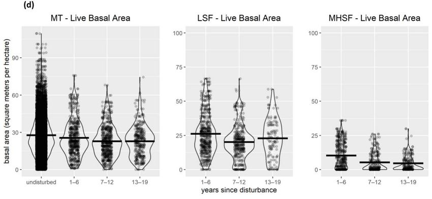
Forests 2021, 12, 150                                                                                            5 of 24

                        retain canopy structures when fires occurred. Post-treatment surface fuels were frequently
                        piled and burned, and occasionally sites were treated with low-severity broadcast burning.
                              We recorded the year in which the silvicultural activity was reported as completed in
                        the FACTS database, and since activities did not occur uniformly within the FACTS GIS
                        polygons (and occasionally we found details within the database were not accurate), we
                        verified that changes in vegetation occurred by comparing records to time-stamped aerial
                        imagery in Google Earth. The mechanical treatment activities were easily visible in the
                        imagery, and if no changes to the forest structure at a given survey station were visible
                        near the dates reported in FACTS, then we did not include that station in the mechanically
                        treated subsample. If we could verify that visible changes to the vegetation were present
                        and consistent with the FACTS database, then we assumed those management activities
                        had occurred as described in the database and we included that station in the mechanical
                        treatment subsample. If the vegetation changes occurred more than 100 m from the survey
                        station location, we did not include that station in the mechanical treatment subsample.
                        If a station received multiple treatments prior to bird surveys, we started the time since
                        treatment count from the last treatment event, and if treated during survey years (2010–
                        2019), we restarted the time since treatment count from that year. Similarly, we identified
                        all stations within a fire perimeter and sampled the vegetation burn severity (assessed as
                        canopy cover % change) at each location and grouped all stations that were burned with less
                        than 25% canopy cover change as low-severity fire and over 25% as moderate-high-severity
                        fire, again verifying all locations identified as burned with aerial imagery in Google Earth.
                        All locations that were mechanically treated (salvage logging or fuels or other vegetation
                        removals) following a fire were removed from analyses. We also removed all data from the
                        year in which a fire or treatment occurred (i.e., time since disturbance cannot be less than 1).
                        All locations with no FACTS or fire disturbance history were included in the undisturbed
                        subsample. We also noted whether each station was located within a clearcut visible on
                        aerial photographs going back to 1980 and included those data in the bird abundance
                        models to account for recent silvicultural treatment history beyond the records contained
                        in the FACTS database that could profoundly influence the avian community decades later.
                        Sample sizes varied by treatment category: moderate-high-severity fire = 217 point count
                        stations on 56 transects, 1144 location-year sampling units; low-severity fire = 197 point
                        count stations on 70 transects, 1094 location-year sampling units; mechanical treatment:
                        275 point count stations on 99 transects, 1584 location-year sampling units; and undisturbed:
                        1542 point count stations on 350 transects, 11,391 location-year sampling units. The sample
                        was dominated by the undisturbed treatment class, a very small portion of which may have
                        been burned or mechanically treated locations that were not captured by the treatment
                        tracking data we used or that we were unable to verify with aerial imagery.

                        2.3. Field Surveys
                             We used standardized five-minute unlimited-distance point count surveys [72,73]
                        to sample the avian community during the peak of the breeding season. At each survey
                        station, we recorded all birds detected (visually or audibly) and estimated their distance
                        to the nearest 1 m from the observer. We visited each station up to twice between 1 May
                        and 15 July in 2010 through 2017, and in 2019. Our field survey project received reduced
                        funding starting in 2017, and we only surveyed half the full sample in 2017 and 2019 and
                        no locations in 2018. The average number of visits per station was 11.9 across the nine years
                        of surveys, or 1.6 surveys per year per point count station. We completed counts within
                        four hours of sunrise and did not survey during inclement weather. Prior to conducting
                        point counts, all observers completed an intensive two-week training program and passed
                        a double-observer field test of bird identification. At each station, we characterized the
                        vegetation within 50 m of the survey plot center using visual estimates of the percentage of
                        the plot that was covered by trees and shrubs (shrub cover includes all understory woody
                        vegetation species), counted standing snags >10 cm diameter, and measured structural
                        characteristics, including the live-tree basal area using a 10-factor key from at least three
Forests 2021, 12, 150 6 of 24
locations within the survey plot [65]. These relevé vegetation surveys were conducted up
to three times at each point count station across the 10-year time span of bird surveys. We
used the vegetation measurements to characterize the progression of vegetation change
over time within each treatment type and used violin plots [74] to show changes over time
within each treatment category, including the mean values of each subsample.
2.4. Bird Abundance Analyses
We recorded a total of 148 species over nine years of surveys on these sites, but for these
analyses, we removed species such as raptors, waterfowl, nocturnal species, detections not
identified to species, and non-breeding migrants for which our point count methodology
generated an inappropriate sample [72]. We further removed all species with fewer than
99 individuals detected within 100 m of observers across all survey events. The remaining
78 species were included in hierarchical distance models to estimate abundance at each
location-year sampling unit using the distsamp function in the Unmarked package [75]
with statistical package R version 3.3.1 [76]. Seven of the 78 species had models that fit the
data overall but had one or more parameters (described below) with very large standard
errors, so we dropped those species from result summaries, leaving a final total of 71 species
for which we show results. These 71 species represented 98% of all individuals detected
in this dataset. See Supplementary Table S1 for a list of species included in the analyses,
common and scientific names, four-letter American Ornithologigal Society codes, total
number of detections, foraging and nesting guilds, and nest types.
To characterize the responses of a large group of species to an unbalanced sample
of a wide variety of vegetation disturbances over a long time period, we took the ap-
proach of fitting abundance models to establish covariate relationships and then used
simplified summaries of vegetation and environmental conditions to project abundances
for each species over time in each disturbance type. We chose this approach so that we
could directly compare the effects of those disturbances, while reducing the influence
of habitat variation and unbalanced sample sizes in the different disturbance types. To
construct the abundance models, we used a stacked-years data structure such that each
site-by-year combination was treated as an independent sampling unit [77,78]. Although
the abundance at a point count location in a given year is not fully independent from
the abundance at the same point in other years, this data structure treats the abundance
state at each point as completely open to colonization or extinction between years, which
may mimic actual ecological processes of rapidly changing conditions following distur-
bance better than assuming closed populations across years. It also makes parameterizing
the vegetation and blocking variables in the model more straightforward than modeling
yearly site extinction and colonization processes directly. These benefits come at the cost
of potentially underestimating the error in some model parameter coefficients. However,
because we are primarily interested in estimating abundances rather than testing hypothe-
ses about covariate influences, we feel that this data structure is warranted and does not
bias our conclusions. To maintain a representative number of sampling units within each
yearly time-since-disturbance category, we capped both burned and mechanical treatment
subsamples at 20 years since disturbance for model-fitting data since sample sizes were
substantially smaller beyond that time period (even though our disturbance history records
included up to 30 years for fires and up to 23 years for FACTS). Finally, we removed all
data from the year in which disturbances occurred (=0 years post-disturbance) from the
model-fitting data, and additionally we did not summarize projected abundances for 1 or
20 years post-disturbance in order to remove some extreme values at the ends of the time
range for some species.
For each species, we fit a single set of model covariates (described below). In addition
to field measurements of the vegetation structure, we included several other variables to
account for geography, climate, and topography. We sampled elevation, aspect, and slope
at each station center from the Sierra Nevada Regional Digital Elevation Model [79]. We
included three additional variables to account for the influence of a widespread droughtForests 2021, 12, 150 7 of 24
throughout the region from 2012 to 2015. Two of these were weather-related variables, and
another represented the amount of tree mortality as a result of drought-induced beetle
infestations [78]. The climatic water deficit (CWD, a measure of water stress based on
evapotranspiration, solar radiation, and air temperature) and a temperature index that
characterizes the average June maximum temperature compared to a 2009 baseline were
sampled using the California basin characterization model (270 m resolution, [80–82]). Tree
mortality was calculated using an index [83] based on the normalized difference wetness
index (NDWI, [84]) using freely available LANDSAT imagery in Google Earth Engine
(see [78] for further details on these methods).
The detection process was modeled using a multinomial function:
Multinomial(Ni ,π i,j ) = α0i + αslope *X1i + αliveBA *X2i + αshrub *X3i
where detection probability (π) varies by location i in distance class j with slope (α_slope),
live-tree basal area (α_liveBA), and percentage shrub cover (α_shrub) included as covariates
in the half-normal (with scale parameter σ) detection function.
Abundance at location i was modeled as a Poisson function assuming closure within
each year and including an offset for the number of visits:
Ni ~Poisson(λi ) = β0i + βelev *X1i + βelev 2 *X2i + βlat *X3i + βelev*lat *X4i + βsouth *X5i +
βCWD *X6i + βmort *X7i + βCWD*lat *X8i + βshrub *X9i + βtree *X10i + βsnags *X11i +
βclearcut *X12i + βMHSF*YSF *X13i + βLSF*YSF *X14i + βMT*YSM *X14i + βMHSF*YSF 2 *X16i +
βLSF*YSF 2 + βMT*YSM 2 *X18i + offset(log(visits))
Covariates in the abundance portion of the model included variables to account for the
highly variable landscape and topography, namely elevation (βelev ), quadratic of elevation
(βelev 2 ), latitude (βlat ), interaction between elevation and latitude (βelev*lat ), and southness
(i.e., aspect represented as a proportion of south-facing (βsouth ). We also included the
vegetation structure covariates shrub cover (βshrub ), tree cover (βtree ), snag density (βsnags ),
and a binary variable indicating whether each location was within a ~1980–1995 clearcut
patch (βclearcut ) to account for recent profound silvicultural management that preceded
the FACTS data. Three variables to account for recent drought conditions were also in-
corporated, climatic water deficit (βCWD ), temperature index (βtemp ), mortality (βmort ),
plus an interaction between climatic water deficit and latitude (βCWD*lat ). Finally, the
model included variables designed to quantify the influence of the three treatment types
(MHSF = moderate-high-severity fire, LSF = low-severity fire, and MT = mechanical treat-
ment) that we described above and to allow for the influence of those treatments on each
species to vary over time. For these variables, we included the interaction between a
treatment-type binary variable (=1 where the treatment or fire occurred and =0 elsewhere)
and the number of years since fire (YSF) or mechanical treatment (YSM) occurred. Treat-
ment was modeled as a linear variable proportional to time since treatment (βMHSF*YSF ),
(βLSF*YSF ), and (βMT*YSM ), as well as their quadratic effects to account for non-linear associ-
ations (e.g., to fit species with the highest or lowest abundances at intermediate values of
time, or abundances that plateau at intermediate values).
All continuous-scale covariates, including time since disturbance, were standardized
(mean = 0.0, standard deviation = 1.0) prior to calculating the squared terms (thus the
quadratic terms have high values for both high and low elevations and low values for
elevations near the mean). We examined the degree of collinearity between vegetation,
topography, and climatic variables using the vif function in the R package HH [85] to calcu-
late variance inflation factors (VIF) and found no evidence of a high degree of collinearity
(all VIF < 3.0). Since the live-tree basal area was moderately correlated with both tree cover
(R = 0.57) and shrub cover (R = 0.38), we only included the live-tree basal area as a detection
covariate. We selected the live-tree basal area for the detection model because we felt it
was the most proximate vegetation feature that influences the observers’ ability to hear
bird vocalizations and visually detect individuals.Forests 2021, 12, 150 8 of 24
To evaluate the differences in abundance for each species between characteristic undis-
turbed, burned, or mechanically treated locations, we used the fitted models to predict
abundance within each treatment category across a broad range of time since disturbance
(2–19 years) with a set of characteristic covariate values derived from averages across
time within each disturbance type (see Figure 2 for a summary of field measurements
and Figure A1 for summarized vegetation covariate values used in predicted abundance
models). Covariates for these predictions included overall mean values (set to zero for
standardized variables) for latitude, elevation, slope, southness, live-tree basal area, mor-
tality, CWD, and temperature index. For the vegetation covariates, we used the mean
yearly value for each of tree cover, shrub cover, and snag density within each disturbance
type to represent the characteristic vegetation conditions and reflect typical changes over
time (Figure A1), and we chose three sets of covariate values that represent three common
undisturbed forest conditions: (1) undisturbed dense forest (high tree cover, low shrub
cover, low snags); (2) undisturbed open forest (low tree cover, low shrub cover, low snags);
and (3) undisturbed shrub-dominant montane chaparral (low tree cover, high shrub cover,
low snags). From the predicted abundances of each species at each time/disturbance-
type combination, we compared the estimates at 2–6 years, 7–12 years, and 13–19 years
post-disturbance to the predicted, 5%, and 95% confidence interval values for each of the
undisturbed types using a t-test (two-tailed, unequal variance) to assess the differences in
abundance between habitats. From those comparisons, we evaluated whether each species
reached its highest abundance within one of the disturbance/time categories or one of
the undisturbed habitat types. As a general summary of community-level adaptations to
disturbance types, we assessed whether each species was consistently more or less abun-
dant in each of the disturbance categories across the entire time range in comparison to the
undisturbed types and summed the number of species that are more abundant (+), less
abundant (-), or not different in abundance (0) in each of the disturbance types (Table S1).
We report the summed total abundance of all species across time since disturbance for
each disturbance type in comparison to the three undisturbed types and also calculate the
inverse Simpson’s diversity metric with the R package Vegan [86], also known as Simpson’s
dominance, which is an index that increases intuitively as diversity increases and reflects
the effective number of species present in a sample [87].
Finally, we quantified the dissimilarity of the bird communities within the treatment
and time categories using the anosim function [86], which provided a comprehensive
statistical test of the pairwise dissimilarity between each of the disturbance and undisturbed
types and highlighted the species that contribute to those dissimilarities. We plotted the
average pairwise dissimilarity for groups of points including the undisturbed types as
well as the entire range of time across the three disturbance types, and repeated the same
analysis after splitting the disturbance types into groups of time of 2–6 years, 7–12 years,
and 13–19 years since the disturbance event. We also identified the species that had the
largest similarity contrasts (contribution to total dissimilarity ≥ 0.002 and abundance at
least 50% larger in one group compared to another) to show which species contribute most
to differences in community composition between habitat types.Forests 2021, 12, 150 9 of 24
Figure 2. Cont.
1Forests 2021, 12, 150 10 of 24
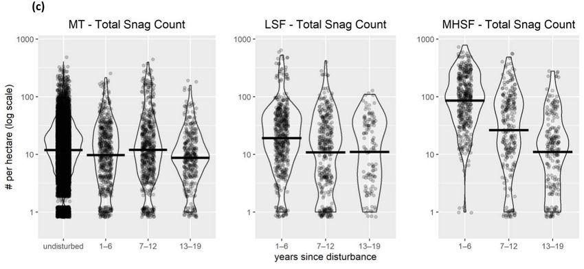
Figure 2. Vegetation measurements at field survey locations within each disturbance type, and sum-
marized across three time periods, in comparison to all undisturbed locations. Vegetation measures
(also used as covariates in abundance models) include (a) shrub cover, (b) tree cover, (c) snag density,
and (d) basal area. Violin plots show mean values as a bold horizontal line. MHSF = moderate-high-
severity fire; LSF = low-severity fire; MT = mechanical treatment; UO = undisturbed open forest;
US = undisturbed shrub; UD = undisturbed dense forest.
3. Results
3.1. Vegetation Changes Following Disturbance
Although there was variability within disturbance categories, each disturbance type
resulted in characteristic patterns of vegetation change and recovery over time (Figure 2).
The mean tree cover within mechanical treatment locations was similar to undisturbed
locations and stayed similar for 19 years after treatments (Figure 2a). Initially following
disturbance, the tree cover in low-severity fire locations was similar to mechanical treatment
locations but declined modestly in the later period. In the first 12 years following moderate-
high-severity fire, the tree cover was much lower and only began to increase after 13 years.
The shrub cover reduced in the first 6 years following mechanical treatment, but over
19 years, there was little difference compared to undisturbed locations (Figure 2b). The
shrub cover was lower immediately after low-severity fire and moderate-high-severity fire
and increased over time, but the increase was more rapid and reached a much higher level
after moderate-high-severity fire. Snags were somewhat rare in undisturbed, mechanical
treatment, and low-severity fire locations and more abundant in moderate-high-severity
fire locations through the first 12 years but then decreased rapidly such that 13–19 years
post-disturbance, the snag density was similar to undisturbed levels (Figure 2c). The
live-tree basal area was lower following moderate-high-severity fire but declined only
slightly following mechanical treatment and low-severity fire and was similar overall to
undisturbed locations (Figure 2d).
3.2. Bird Abundance and Response to Disturbance
Patterns of total bird abundance varied between disturbance types and over time
(Figure 3). Immediately following disturbance, bird abundance was the highest in mechan-
ical treatment but then steadily declined over time, such that by the end of the time period,
it supported the second-lowest total abundance. In contrast, abundance in moderate-
high-severity fire locations was far lower immediately following disturbance compared to
2
undisturbed or the other two disturbance types. However, it increased rapidly in the two
decades following disturbance such that it equaled the undisturbed levels and was higher
than the other two disturbance types. Low-severity fire locations were initially similar in
abundance to the undisturbed types but declined over time to the lowest value overall.Forests 2021, 12, 150 11 of 24
Forests 2021, 12, x FOR PEER REVIEW 11 of 24
Figure 3. Total abundance (sum of all individuals across all species) over time. Abundance
mates were generated for each species within each disturbance type projected from charac
vegetation values for tree cover, shrub cover, and snags (Figure A1), while holding all oth
parameters constant. Error bars show the sum of 5% and 95% CIs for each species’ abunda
mate. MHSF = moderate-high-severity fire; LSF = low-severity fire; MT = mechanical treatm
Figure
UO = 3.undisturbed
Figure 3.Total
Totalabundance (sum
abundance
open of all
(sum ofindividuals
forest; all
US acrossacross
individuals all species)
= undisturbed all overUD
time.
species)
shrub; =Abundance
over esti- dense
time. Abundance
undisturbed esti-
forest.
mates were
mates weregenerated
generated forfor
each species
each species within eacheach
within disturbance type projected
disturbance from characteristic
type projected from characteristic
vegetation values for tree cover, shrub cover, and snags (Figure A1), while holding all other model
vegetation values for tree cover, shrub cover, and snags (Figure A1), while holding all other model
A different
parameters pattern
constant. Error emerges
bars show the sum of when
5% andconsidering
95% CIs for eachdiversity among
species’ abundance esti-the different
parameters
mate. MHSF constant. Error bars show
= moderate-high-severity fire; the
LSFsum of 5% and
= low-severity 95%
fire; MTCIs for each species’
= mechanical treatment; abundance
ance types
estimate. MHSF(Figure
UO = undisturbed =open 4). Moderate-high-severity
moderate-high-severity
forest; US = undisturbed fire;shrub;
LSF =UD low-severity firefire;
= undisturbed
locations
MT =forest.
dense
had far
mechanical higher dive
treatment;
the=first
UO 13 years
undisturbed open post-disturbance,
forest; US = undisturbedpeaking shrub; UD in year 13, dense
= undisturbed but then forest.precipitously d
suchA that
different
thepattern
otheremerges when considering
two disturbance types diversity
supported among equalthe different disturb-diversity by
or higher
ance A different
types (Figurepattern emerges when considering
4). Moderate-high-severity diversity
fire locations had far among
higher the different
diversity fordistur-
post-disturbance.
bance This decrease in diversity coincided
the first 13 years post-disturbance, peaking in year 13, but then precipitously declined, for
types (Figure 4). Moderate-high-severity fire locations had with
far higher a large
diversity increase in t
birdfirst
the
such abundance,
that 13
theyears twowhich
other post-disturbance,wastypes
disturbance driven
peaking byinayear
supported relatively
equal13,orbut small
then
higher number
precipitously
diversity ofdeclined,
by 19 years primarily shru
ciated
such thatspecies
the other
post-disturbance. (e.g.,
two
This sparrows).
disturbance
decrease Low-severity
types
in diversity supported
coincided with firea locations
equal or higher
large initially
diversity
increase in theby had much lowe
19 years
total
bird abundance,
post-disturbance. which
This was driven
decrease in by a relatively
diversity small
coincided
sity than moderate-high-severity fire locations but increased over time number
with a of
largeprimarily
increase shrub-asso-
in the total birdsuch th
ciated specieswhich
abundance, (e.g., sparrows).
was driven Low-severity
by a relatively fire locations
small number initially
ofhad much lower
primarily diver-
shrub-associated
years
sity thanpost-disturbance,
species moderate-high-severity
(e.g., sparrows). Low-severity
low-severity
fire locations fireincreased
but
fire locations
areas supported
overhad
initially timemuch thethat
such highest
lower 19 bird diver
bydiversity
versity
than in mechanical
years moderate-high-severity treatment
post-disturbance, low-severity locations
fire areasbut
fire locations was
supported
increased initially
theover
highesttime the
bird lowest
diversity.
such of
that byDi- 19all disturban
years
versity in mechanical
but increased
post-disturbance, treatmentacross
modestly
low-severity locations
fire areas was
time. initially the
Diversity
supported the lowest
wasofhigher
highest all
birddisturbance
in all types
diversity. three
Diversitydisturban
butmechanical
in increased modestly
treatment across time. Diversity
locations was was higher
initially the in all of
lowest three
all disturbance
disturbance types
types but
across all time
across all time
periods
periods than the
than
two
the two undisturbed
undisturbed
forest types but generally lower
increased modestly across time. Diversity was forest
highertypesin allbut generally
three lower than
disturbance types inacross
theshrub-dominated
the shrub-dominated undisturbed
undisturbed type. Undisturbed
type. Undisturbed shrub had far higher shrub had far
diversity than higher divers
all time periods than the two undisturbed forest types but generally lower than in the
the undisturbed
the undisturbed
shrub-dominated
forest forest types
types
undisturbed
and was and was similar
similar
type. Undisturbed
to to far
moderate-high-severity
moderate-high-severity
shrub had higher diversity than the fire l
fire locations
overall.
overall. forest types and was similar to moderate-high-severity fire locations overall.
undisturbed
Figure 4. Inverse Simpson’s diversity calculated from modeled species abundance estimates pro-
jected over time. Modeled abundance estimates were generated for each species within each dis-
turbance type projected from characteristic vegetation values for tree cover, shrub cover, and
snags (Figure A1), while holding all other model parameters constant. Error bars show the diver-
sity of 5% and 95% Simpson’s
CIs for species’ abundance estimates. MHSF = moderate-high-severity fire; LSF pro-
Figure4.4.Inverse
Figure Inverse Simpson’s diversity calculated
diversity from
calculatedmodeled
from species
modeled abundance
speciesestimates
= low-severity fire; MT = mechanical treatment; UO = undisturbed open forest; US = undisturbed
abundance estimat
jected over time. Modeled abundance estimates were generated for each species within each dis-
jectedUD
shrub; over time. Modeled
= undisturbed abundance estimates were generated for each species within ea
dense forest.
turbance type projected from characteristic vegetation values for tree cover, shrub cover, and snags
turbance type projected from characteristic vegetation values for tree cover, shrub cover, a
(Figure A1), while holding all other model parameters constant. Error bars show the diversity of
snags (Figure A1), while holding all other model parameters constant. Error bars show the
5% and 95% CIs for species’ abundance estimates. MHSF = moderate-high-severity fire; LSF = low-
sity of 5% and 95% CIs for species’ abundance estimates. MHSF = moderate-high-severity
severity fire; MT = mechanical treatment; UO = undisturbed open forest; US = undisturbed shrub;
= low-severity
UD = undisturbedfire; MT
dense = mechanical treatment; UO = undisturbed open forest; US = undis
forest.
shrub; UD = undisturbed dense forest.Forests 2021, 12, 150 12 of 24
The species’ responses to disturbances that contribute to these patterns were highly
varied, but some broad patterns did emerge (Table S2). There were 21/71 species that
declined following moderate-high-severity fire in comparison to their abundance in undis-
turbed locations. These species were largely associated with mature forests and were
among the most abundant species in our study area (e.g., red-breasted nuthatch, yellow-
rumped warbler, hermit warbler). However, the majority of the community (38/71) had
higher abundances following moderate-high-severity fire, including 10 species that were
more than twice as abundant in moderate-high-severity fire locations than any other distur-
bance or undisturbed type. Most of these moderate-high-severity fire-dependent species
were among the rarer species in the community, such as yellow warbler, lazuli bunting,
mountain and western bluebird, house wren, and black-backed woodpecker. All of the
species that were far more abundant in moderate-high-severity fire locations are either
shrub or snag associates (Tables S1 and S2). Most species in the community were also
largely tolerant of low-severity fire and mechanical treatment, with 50/71 species having
little to no difference in abundance in either of these disturbance types compared to undis-
turbed, and 16/71 in both disturbance types having higher abundance. Nine of the ten
most abundant species in our study area were not significantly different in abundance
following low-severity fire or mechanical treatment compared to undisturbed locations.
In comparing the time and disturbance-type combinations at which each species
was predicted to reach its maximum abundance, we again found much variation and a
few general patterns. There were relatively few species that had the highest abundances
in undisturbed types (13/71) in comparison to the disturbance types (Table S2). More
species (34/71) were predicted to reach peak abundance in moderate-high-severity fire
than in mechanical treatment (16/71) or low-severity fire (8/71) locations. In addition, the
species that reached peak abundance in moderate-high-severity fire locations tended to
be among the moderate and less abundant species, while those that peaked in mechanical
treatment locations tended to be among the most abundant. Species were also mostly
predicted to occur at peak abundance in either extreme of the timescale, with those peaking
in mechanical treatment locations somewhat evenly split among the early and late time
periods and those in moderate-high-severity fire locations generally peaking during the
later time period (13–19 years since disturbance; 22/34 species).
When we considered life history traits, such as nest substrate and foraging strategy, of
these species, some clear patterns emerged. Of the ground- and shrub-nesting species, the
majority (22/32) reached peak abundance in moderate-high-severity fire locations, with
the rest were evenly spread among the other conditions. Ten of the nineteen cavity-nesting
species reached the highest abundance in moderate-high-severity fire locations, with two
others in low-severity fire locations, three in mechanical treatment locations, and four
in undisturbed habitats. Of the 28 tree-nesting species, 10 reached peak abundance in
mechanical treatment locations, 7 in moderate-high-severity fire (generally earlier post-
disturbance), 6 in undisturbed dense forest, and 5 in low-severity fire locations. Among
foraging strategies, two of the three bark-drilling woodpeckers reached peak abundance in
moderate-high-severity fire locations; bark gleaners were spread evenly among the other
conditions. Of the 25 omnivore and seed-consuming species, 15 reached peak abundance
in moderate-high-severity fire locations. Fourteen of the thirty-three foliage, ground, and
aerial insectivores reached peak abundance in moderate-high-severity fire locations, with 4
in low-severity fire, 6 in mechanical treatment, and 9 in undisturbed habitats.
3.3. Community Similarity
Similarity analysis revealed that moderate-high-severity fire locations provide habitats
for a unique component of the bird community, having the largest dissimilarities in species
composition in comparison to other disturbance types, with undisturbed dense forest
being the next largest, and low-severity fire, mechanical treatment, undisturbed shrub,
and undisturbed open forest locations having comparable and smaller dissimilarities on
average (Figure 5 and Table S2). The smallest dissimilarity was between undisturbedForests 2021, 12, x FOR PEER REVIEW 13 of 24
Forests 2021, 12, 150 13 of 24
shrub, and undisturbed open forest locations having comparable and smaller dissimilari-
ties on average (Figure 5 and Table S2). The smallest dissimilarity was between undis-
open forest
turbed openand undisturbed
forest dense forest,
and undisturbed dense followed by low-severity
forest, followed fire andfire
by low-severity mechanical
and me-
treatmenttreatment
chanical locations.locations.
Comparing the bird communities
Comparing between groups
the bird communities betweenof points
groupsdefined by
of points
both time
defined byand
bothdisturbance categories showed
time and disturbance thatshowed
categories the mostthat
unique bird communities
the most were
unique bird com-
found early
munities were(2–6 years)
found after
early moderate-high-severity
(2–6 fire and especially
years) after moderate-high-severity afterespecially
fire and 13–19 years
af-
(Figure 5). The smallest dissimilarities occurred between habitats in the
ter 13–19 years (Figure 5). The smallest dissimilarities occurred between habitats 7–12 years’ time
in the 7–
period,
12 years’especially for low-severity
time period, especially forfire and mechanical
low-severity fire andtreatment locations.
mechanical treatment locations.
Figure 5. Dissimilarity across all pairwise combinations of disturbance/time categories and undis-
turbed 5.habitat
Figure types (total
Dissimilarity acrosspairwise comparisons,
all pairwise n = of
combinations 11). Horizontal bars
disturbance/time show group
categories means.
and undis-
turbed
MHSF =habitat types (total pairwise
moderate-high-severity fire;comparisons, n = 11).
LSF = low-severity Horizontal
fire; bars show
MT = mechanical group means.
treatment; UO = undis-
MHSF
turbed=open
moderate-high-severity fire; LSF
forest; US = undisturbed = low-severity
shrub; fire; MT = dense
UD = undisturbed mechanical
forest.treatment;
NumbersUO =
indicate
undisturbed open
ranges of years forest;
since US = undisturbed shrub; UD = undisturbed dense forest. Numbers indi-
disturbance.
cate ranges of years since disturbance.
The species that accounted for the largest portion of each dissimilarity comparison
The species
included a groupthat accounted
of mature for the largest species
forest-associated portion(golden-crowned
of each dissimilarity comparison
kinglet, yellow-
included a groupred-breasted
rumped warbler, of mature forest-associated
nuthatch, Hammond’s species (golden-crowned
flycatcher, and hermitkinglet,
warbler,yellow-
among
rumped
others; see warbler, red-breasted
Table S3). These maturenuthatch,
forestHammond’s
species wereflycatcher,
more abundant and hermit warbler,
in undisturbed
among others;
dense forest andseeundisturbed
Table S3). These
openmature
forest inforest species were
comparison more abundant in undis-
to moderate-high-severity fire,
turbed
and also in undisturbed dense forest in comparison to undisturbed moderate-high-severity
dense forest and undisturbed open forest in comparison to shrub habitats. A group
fire, and also
of shrub and in undisturbed
open dense also
habitat species forest in comparison
appeared to undisturbed
to be driving shrub habitats.
the dissimilarity between A
group of shrub and open
moderate-high-severity habitat
fire species alsoshrub
and undisturbed appeared to beindriving
locations comparisonthe dissimilarity
to undisturbed be-
tween
dense moderate-high-severity
forest, undisturbed openfire and undisturbed
forest, and mechanical shrub locations
treatment in comparison
locations to un-
(fox sparrow,
disturbed
house wren, dense forest,
yellow undisturbed
warbler, open forest,towhee,
and green-tailed and mechanical treatmentThere
among others). locations
were(fox no
species with
sparrow, strong
house contributions
wren, to dissimilarity
yellow warbler, between low-severity
and green-tailed towhee, among fire and mechanical
others). There
treatment
were or between
no species undisturbed
with strong dense forest
contributions and undisturbed
to dissimilarity between open forest locations.
low-severity fire and
mechanical treatment or between undisturbed dense forest and undisturbed open forest
4. Discussion
locations.
Following a century of fire suppression, the concomitant natural disturbance deficit
inDiscussion
4. many frequent-fire forests, recent large increases in area burned at high severity, and
renewed calls for
Following increasing
a century forest
of fire resilience,the
suppression, it is important to
concomitant understand
natural the broader
disturbance deficit
ecological effects of different disturbance agents that could potentially
in many frequent-fire forests, recent large increases in area burned at high severity, be used to restore
and
these forests. We found large differences in the composition and abundance
renewed calls for increasing forest resilience, it is important to understand the broader of the avian
community
ecological among
effects of disturbance types across
different disturbance the first
agents that 20 years
could followingbe
potentially disturbance.
used to restoreThe
conditions that supported the highest abundance and diversity
these forests. We found large differences in the composition and abundance of the avian of avian species varied
across the post-disturbance period. Overall, far more species reached peak abundance
community among disturbance types across the first 20 years following disturbance. The
following some form of disturbance than in forests that had not been disturbed in the
conditions that supported the highest abundance and diversity of avian species varied
past 20 years. In this current state of homogenized, smaller-diameter, and overly dense
across the post-disturbance period. Overall, far more species reached peak abundance fol-
forest stands created through decades of intensive logging and fire suppression within this
lowing some form of disturbance than in forests that had not been disturbed in the past
region [88,89], the importance of disturbance to the avian community is very apparent.
20 years. In this current state of homogenized, smaller-diameter, and overly dense forest
However, the relatively low dissimilarity between mechanical treatment areas, low-severity
stands created through decades of intensive logging and fire suppression within this re-
fire areas, and undisturbed forests suggest that from an avian community perspective,
gion [88,89], the importance of disturbance to the avian community is very apparent.
these disturbances do not bring about ecologically meaningful changes to the system.
Our findings do highlight the unique contribution that moderate-high-severity fire has inYou can also read