FORCE MAJEURE The Sun's Role in Climate Change Henrik Svensmark - The Global Warming Policy Foundation - GWPF
←
→
Page content transcription
If your browser does not render page correctly, please read the page content below
FORCE MAJEURE
  The Sun’s Role in Climate Change
  Henrik Svensmark

The Global Warming Policy Foundation
GWPF Report 33
FORCE MAJEURE
The Sun’s Role in Climate Change
Henrik Svensmark

ISBN 978-0-9931190-9-5
© Copyright 2019 The Global Warming Policy Foundation
Contents

   About the author                                              vi
   Executive summary                                             vii
   1   Introduction                                               1
   2   The sun in time                                            1
       Solar activity                                             1
       Solar modulation of cosmic rays                            3
       Reconstructed solar irradiance                             4
   3   Correlation between solar activity and climate on Earth    6
   4   Quantifying the link between solar activity and climate   10
   5   Possible mechanism linking solar activity with climate    11
       Total solar irradiance and temperature                    11
       UV changes and temperature                                12
       Cosmic rays, clouds and climate                           12
       Changes in the Earth’s electrical circuit                 16
   6   Future solar activity                                     17
   7   Discussion                                                17
       Impact of solar activity                                  18
       Solar UV mechanism                                        19
       Cosmic ray clouds mechanism                               19
       Electric field mechanism                                  20
   8   Conclusion                                                20
   9   Appendix: A simple ocean model calculation                22

Bibliography                                                     25
About the author Henrik Svensmark (born 1958) is a physicist and a senior researcher in the Astrophysics and Atmospheric Physics Division of the National Space Institute (DTU Space) in Lyngby, Den- mark. In 1987, he obtained a PhD from the Technical University of Denmark and has held postdoctoral positions in physics at three other organizations: the University of California, Berkeley, the Nordic Institute for Theoretical Physics, and the Niels Bohr Institute. Henrik Svensmark presently leads the Sun–Climate Research group at DTU Space. Acknowledgement I thank Lars Oxfeldt Mortensen, Nir Shaviv and Jacob Svensmark and two reviewers for con- tributing helpful comments to this manuscript. vi
Executive summary
Over the last twenty years there has been good progress in understanding the solar influ-
ence on climate. In particular, many scientific studies have shown that changes in solar activ-
ity have impacted climate over the whole Holocene period (approximately the last 10,000
years). A well-known example is the existence of high solar activity during the Medieval
Warm Period, around the year 1000 AD, and the subsequent low levels of solar activity during
the cold period, now called The Little Ice Age (1300–1850 AD). An important scientific task
has been to quantify the solar impact on climate, and it has been found that over the eleven-
year solar cycle the energy that enters the Earth’s system is of the order of 1.0–1.5 W/m 2 . This
is nearly an order of magnitude larger than what would be expected from solar irradiance
alone, and suggests that solar activity is getting amplified by some atmospheric process.
    Three main theories have been put forward to explain the solar–climate link, which are:
     • solar ultraviolet changes
    • the atmospheric-electric-field effect on cloud cover
     • cloud changes produced by solar-modulated galactic cosmic rays (energetic particles
       originating from inter stellar space and ending in our atmosphere).
Significant efforts has gone into understanding possible mechanisms, and at the moment
cosmic ray modulation of Earth’s cloud cover seems rather promising in explaining the size of
solar impact. This theory suggests that solar activity has had a significant impact on climate
during the Holocene period. This understanding is in contrast to the official consensus from
the Intergovernmental Panel on Climate Change, where it is estimated that the change in
solar radiative forcing between 1750 and 2011 was around 0.05 W/m 2 , a value which is en-
tirely negligible relative to the effect of greenhouse gases, estimated at around 2.3 W/m 2 .
However, the existence of an atmospheric solar-amplification mechanism would have im-
plications for the estimated climate sensitivity to carbon dioxide, suggesting that it is much
lower than currently thought.
    In summary, the impact of solar activity on climate is much larger than the official consen-
sus suggests. This is therefore an important scientific question that needs to be addressed
by the scientific community.

                                                                                               vii
1 Introduction
The Sun provides nearly all the energy responsible for the dynamics of the atmosphere and
oceans, and ultimately for life on Earth. However, when it comes to the observed changes
in our terrestrial climate, the role of the Sun is not uniformly agreed upon. Nonetheless, in
climate science an official consensus has formed suggesting that the effect of solar activity
is limited to small variations in total solar irradiance (TSI), with insignificant consequences
for climate. This is exemplified in the reports of Working Group I of the Intergovernmental
Panel on Climate Change (IPCC), who estimate the radiative forcing on climate from solar
activity between 1750 and 2011 at around 0.05 W/m 2 . This value is entirely negligible com-
pared to changes in anthropogenic greenhouse gases, whose forcing is estimated at around
2.3 W/m2 . 1
The aim of this report is to give a review of research related to the impact of solar ac-
tivity on climate. Contrary to the consensus described above, there is abundant empirical
evidence that the Sun has had a large influence on climate over the Holocene period, with
temperature changes between periods of low and high solar activity of the order of 1–2 K.
Such large temperature variations are inconsistent with the consensus and herald a real and
solid connection between solar activity and Earth’s climate. The question is: what is the
mechanism that is responsible for the solar–climate link? A telling result is given by the en-
ergy that enters the oceans over the 11-year solar cycle, which is almost an order of magni-
tude larger (∼1–1.5 W/m2 ) than the corresponding TSI variation (∼0.2 W/m2 ). Solar activity
is somehow being amplified relative to the TSI variations by a mechanism other than TSI.
There are other possible drivers of these changes: solar activity also manifests itself in
components other than TSI. These include large relative changes in its magnetic field, the
strength of the solar wind (the stream of charged particles that carries the magnetic field),
modulation of cosmic ray ionisation in the Earth’s atmosphere, and the amount of ultraviolet
(UV) radiation, to name a few. All of these are part of what is referred to as ‘solar activity’, and
all have been suggested to influence climate as well. In particular, it will be shown that a
mechanism has been identified that can explain the observed changes in climate, and which
is supported by theory, experiment and observation.
This report is not meant to be an exhaustive representation of all the published papers
related to a solar influence on Earth’s climate, but aims to give a clear presentation of the
current knowledge on the link between solar activity and climate. A comprehensive review
of the Sun’s impact on climate was published previously, 2 but is now eight years old; im-
portant progress on the mechanism linking solar activity and climate has been made since.
Technical material will not be included in the report, but rather reference will be made to
the literature in the field so that the interested reader can find further information.
2 The sun in time
Solar activity
One of the lessons from scientific studies of the Sun is that it is highly dynamical, exhibiting
changes on timescales from seconds to millennia. Solar activity is caused by magnetic fields
that are generated by the Sun’s differential rotation and by convection of the solar plasma.
The solar equator rotates faster than the poles: the equator has a period of around 25 days,
compared to around 38 days at the poles. This difference causes the magnetic dipole field
to wind up. Due to the repulsion and lower density of the field lines, they eventually pene-
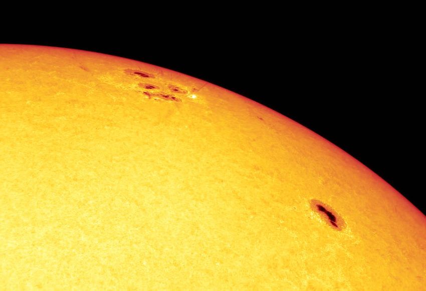
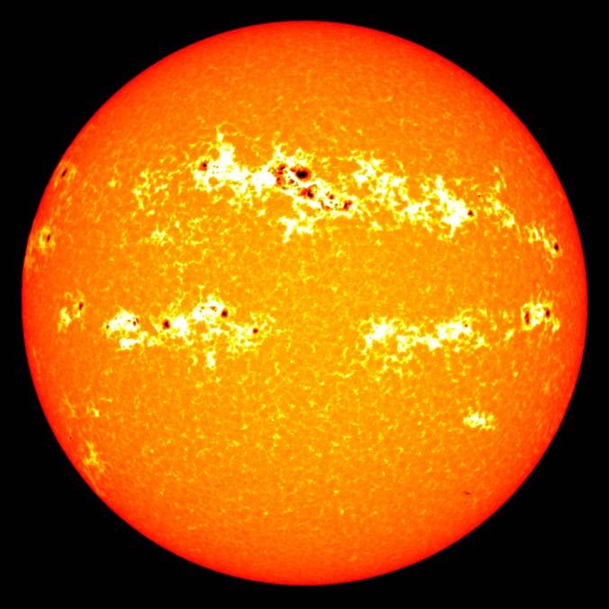
1Figure 1: The Sun during a period of high solar activity.
The colours have been altered to enhance the appearance of the faculae (white regions) which
are hotter than the sunspots (red–black regions). The dark regions associated with sunspots
tend to lower, whereas the brighter regions tend to increase, the solar flux reaching the Earth.
Source: NASA/Goddard Space Flight Center Scientific Visualization Studio.
trate the surface of the Sun – the Photosphere – as what are called ‘sunspots’. These regions
appear dark because the magnetic fields inhibit convection and so they are colder than the
surrounding regions. In addition to sunspots, there are bright regions called ‘faculae’, which
are granular structures on the Sun’s surface that are slightly hotter than the surrounding
photosphere (see Figure 1). The basic variation in sunspots is an activity cycle of about 11
years, which arises from quasi-periodic reversals of the solar magnetic dipole field. Every so-
lar cycle, the number of sunspots increases to a peak, which is known as a ‘solar maximum’.
Then, after a few years of high activity, the Sun will display low activity for a period known
as a ‘solar minimum’.
On longer timescales (from decades to millennia), there are irregular variations in solar
activity that modulate the 11-year sunspot cycle. For example, during the Middle Ages and
during the latter half of the 20th century, the peaks in the 11-year cycles were notably strong,
while they were low or almost absent during the Maunder Minimum (1645–1715) and the
Dalton Minimum (1796–1820), as shown in Figure 2. Here the record of activity is based
on observations of sunspots using a telescope. The record was initiated by Galileo Galilei in
1610 and since that time observations have been performed by numerous observers, result-
ing in a continuous record more than 400 years long.
Of course, the record contains observational bias due to changes in instrumentation and
215
Maunder Minimum
Sunspot group number
Dalton Minimum
10
5
0
1600 1700 1800 1900 2000
Hoyt and Schatten Svalgaard and Schatten Usoskin et al.
Figure 2: Three reconstructions of the sunspot group record.
The sunspot group number is the number of groups of sunspots. Sunspot groups have been
easier to observe in the past since it is not necessary to resolve individual sunspots. Notice that
the quasi-period of 11 years is modulated on longer timescales. Two of the three
reconstructions indicate a secular increase in solar activity since the Maunder Minimum.
Sources: Hoyt and Schatten, covering 1610–1995, 3 Svalgaard and Schatten, covering
1610–2015, 4 and Usoskin et al., 1749–1995. 5
changes in the method of counting sunspots, leading to uncertainty, particularly in the early
part of the record. Figure 2 illustrates this problem. The three reconstructions of the sunspot
group number are shown. It is seen that two of the reconstructions (pink and grey curves)
support the idea of a secular increase in solar activity towards the end of the 20th century. 3,5,6
However, the third reconstruction (blue curve) deviates from the other two by being signif-
icantly and systematically higher in the 18th and 19th centuries. 4 This discrepancy has not
been resolved but, as we shall see, records of changes in cosmogenic isotopes support the
idea of increasing magnetic solar activity up to end of the 20th century.
Solar modulation of cosmic rays
Solar activity modulates cosmic rays, also referred to as galactic cosmic rays. These are very
energetic particles originating from the interstellar medium; in other words, from outside
the solar system. They obtain their energy when they are accelerated by the shock-fronts
from supernovae (stars that ends their lives in violent explosions). When cosmic rays enter
the solar system they have to penetrate the Heliosphere, the region of space that is domi-
nated by the Sun’s magnetic field, carried by the solar wind. Here the cosmic ray particles
get scattered by magnetic fluctuations, a process which screens the inner part of the Helio-
sphere from a large proportion of the particles.
3Cosmic rays consist mainly of protons (90%) and of alpha-particles (9%), plus a smaller
proportion of heavier components. Their energies range between a few million electron
volts (eV) and 1020 eV; as the energy of the particles increases, they become rarer. Cosmic
rays can be recorded through ground-based neutron monitors, which can detect variations
in the low-energy part of the primary cosmic ray spectrum. The lowest energy that can be
detected at the top of the atmosphere depends on the geomagnetic latitude, and ranges
from 0.01 GeV (1 GeV = 109 eV) at stations near the geomagnetic poles to about 15 GeV near
the geomagnetic equator.
Systematic instrumental monitoring of cosmic rays started after 1950 with the use of
neutron monitors. Figure 3 shows normalised cosmic ray variations for 1951–2006, and the
variation in sunspots over the same period. 7 The cosmic ray intensity exhibits an inverse re-
lationship to the sunspot cycle. This is caused by the magnetic structure of the solar wind in
the interplanetary medium, which has a larger shielding effect on cosmic rays during periods
of high solar activity.
It is, however, possible to obtain information about variations in cosmic rays in the years
before neutron monitors became available. When energetic cosmic rays collide with the
atoms of the atmosphere, new elements are produced. These elements are referred to as
‘cosmogenic isotopes’. Examples are beryllium-10, carbon-14 and chlorine-36. When the
cosmic ray flux is high, the production of cosmogenic isotopes is also high, and vice versa
when the flux is low. Variations in the quantity of cosmogenic isotopes therefore provide
information on the variations in the cosmic-ray flux. For example, beryllium-10 ( 10 Be) is pro-
duced high in the Earth’s atmosphere by cosmic rays. The 10 Be atoms can then stick to small
aerosols (molecular clusters floating in the air), and sometimes they become incorporated
into snowflakes. If these fall somewhere where they will not melt, for example the Greenland
icesheet, then by taking ice-cores and measuring the content of 10 Be atoms in each dated
layer of ice, a record of 10 Be production, and thereby an indirect measure of past cosmic ray
flux, is obtained.
Figure 4 shows such a record: a reconstruction of cosmic rays back to 1391; after 1951
the instrumental record is used. 8 The figure also shows the sunspot group number starting
in 1610. Notice there is a clear inverse correlation between solar activity and cosmic rays
in the period of overlap. However, there are subtle differences. For example, the Maunder
Minimum (1645–1715) had very few sunspots, but the end of the Maunder Minimum (1690-
1715) has the highest cosmic ray flux compared to the rest of the period.
Cosmogenic isotopes can be used to reconstruct the cosmic ray variation for up to 10,000
years back in time, and such indirect reconstructions are called ’proxies’ of cosmic rays or
solar activity. On longer timescales it may be necessary to correct for changes in Earth’s
magnetic field. 8
Reconstructed solar irradiance
Total solar irradiance (TSI) describes the integrated radiant energy arriving from the Sun at
the top of Earth’s atmosphere, and represents nearly all the energy that the Earth receives.
It is therefore an important parameter in Earth’s climate. Since 1978, direct observations of
TSI have been obtained from Earth-orbiting satellites. However, these wear out and have
to be replaced from time to time, so the records from each have to be inter-calibrated to
provide a continuous time series. 9 Due to data gaps and instrument degradation, the precise
calibration needed is not universally agreed upon. 9–11
4110 600
100 500
90 400
Sunspot number
Cosmic rays (%)
80 300
70 200
60 100
50 0
1950 1960 1970 1980 1990 2000 2010 2020
Cosmic rays Sunspot number
Figure 3: Cosmic ray and sunspot variations over the instrumental period (1951–2018).
Sources: Cosmic rays per McCracken and Beer, 8 sunspots per Climax neutron monitor, 7
extended after 2006 by the author using data from the Oulo monitor.
120
80
110
100 60
Sunspot group number
Cosmic rays (%)
90
Maunder Minimum
Dalton Minimum
40
80
20
70
60 0
1400 1500 1600 1700 1800 1900 2000
Cosmic rays Group sunspot number
Figure 4: 10 Be reconstruction of cosmic ray variation since 1391.
There has been a steady decrease in the cosmic rays on long timescales, indicating that the part
of solar magnetic activity responsible for modulating cosmic rays has increased over this
period. Sources: Cosmic rays: McCracken and Beer; 8 sunspot group record, Hoyt et al. 3,6
5An important question concerns if there is a trend in the TSI data beyond the 11-year cy-
cle: this could have implications for estimates of TSI changes on long timescales and thereby
on climate. Satellite data demonstrate that TSI varies by as much as 0.05–0.07% over a solar
cycle. 9–11 At the top of the atmosphere this variation amounts to around 1 W/m 2 out of a so-
lar constant of around 1365 W/m2 . At the surface it is only 0.2 W/m2 , after taking geometry
and albedo into account.
On longer timescales there has been interest in reconstructing TSI beyond the satellite
period by using a number of solar proxies. Typically, the TSI is represented as the sum of
the radiances from three distinct regions of the sun: the bright faculae, the dark sunspots,
and the other areas, known as the ‘quiet Sun’. Past observations of faculae and sunspots can
drive estimates of the first two components, but there is no way to estimate past activity
of the quiet Sun, so it is common to assume a constant level of irradiance. A majority of
reconstructions find only small changes in overall secular solar radiative output: since the
Maunder Minimum, TSI is believed to have increased by around 1 W/m 2 , which corresponds
to 0.18 W/m2 at the Earth’s surface. This is too small to have had an impact on climate. 12,13
In contrast, a few TSI reconstructions suggest a much larger TSI increase since the Maun-
der Minimum (0.4%, or around 6 W/m 2 ). 14,15 These reconstructions are based upon the hy-
pothesis that the quiet solar irradiance has varied significantly over time. The assumption is
that the irradiance from the quiet regions can be parametrised by the solar magnetic field
that modulates the cosmic rays, resulting in large variations in TSI. However, the suggestion
of large variations in the irradiance from the quiet Sun has been severely questioned. 16,17
For example, a test of TSI variations over the 20th century was performed using CaK spectro-
heliograms of the solar disk covering the period 1914–1996. The heliograms showed very
little variation in the magnetic network over the period, an observation which is inconsistent
with large TSI variations. 18,19
If solar activity continues declining over the next few decades it may be possible to better
constrain TSI variations.
3 Correlation between solar activity and climate on Earth
Many empirical studies have shown a clear correlation between proxy measurements of cli-
mate and of solar activity on timescales of decades or longer. In the 1970s, John Eddy no-
ticed a correlation between solar activity and the European climate over the previous mil-
lennium. 20 For example, the Little Ice Age (1300–1850 AD), was a cold period that took place
while the Sun was particularly inactive. The Medieval Warm Period (1000–1200 AD), on the
other hand, occurred while the Sun was active.
Figure 5a shows recent reconstructions of temperature variation over the last 1000 years.
A number of temperature records are compared (with respect to the 1961–1990 average
temperature):
• two multiproxy reconstructions of Northern Hemisphere temperatures 21,22
• a global temperature reconstruction based on borehole temperatures 23
• the instrumental record over the last 150 years. 24
Figure 5b displays cosmic ray reconstructions based on:
14
• C measurements in tree rings1
10
• Be concentrations from
60.5
Medieval Warm Period
Temperature anomaly (◦ C)
0
Little Ice Age
-0.5
-1.0
800 1000 1200 1400 1600 1800 2000
Moberg multiproxy (and 95% confidence int) Instrumental record
Huang boreholes Mann and Jones multiproxy
(a) Temperature anomalies versus 1961–1990 average
-1.0
Maunder
Dalton
Spörer
-4
Oort
Wolf
-0.5Δ10 Be anomaly (arbitrary units)
-2
Δ14 C anomaly (%)
0 0
2
0.5
4
1.0
800 1000 1200 1400 1600 1800 2000
Δ14 C Δ10 Be, (Delaygue and Bard 2011) Δ10 Be, Beer et al. (1994)
(b) Galactic cosmic rays (inverted scale; solar minima are shown in grey)
Figure 5: Temperature and cosmic ray variations over the last millennium.
Note the inverted scale in the lower chart; high cosmic ray fluxes are associated with cold
temperatures. See main text for sources.
7– ice cores from Antarctica. 25
– an ice core from Greenland. 26
10
-3.5
5
-4.0
0
-4.5
Δ14 C
δ 18 O
-5
-10 -5.0
-15
-5.5
6.5 7.0 7.5 8.0 8.5 9.0 9.5
Thousands of years ago
Δ14 C δ 18 O
Figure 6: Remarkable correlation between a temperature proxy and a solar activity proxy.
Temperatures based on δ 18 O in stalagmites in a cave in Oman, reflecting monsoon rainfall.
Solar activity based on δ 14 C. Source: Neff et al. 27
The two parts of the figure show that there is a remarkable correlation between the
changes in temperature and changes in cosmic rays (caused by solar activity). In fact, it is
possible to see all the solar activity minima manifested in the temperature curve. Notice
that the axis for the cosmic ray plot is inverted so that a high cosmic-ray flux corresponds to
colder temperatures and a low cosmic-ray flux to higher temperatures.
One way to show that the solar–climate link is seen globally is to look at the temperature
reconstructions based on worldwide borehole data (Figure 5a, grey curves). Due to the slow
diffusion of heat into the ground, the measured temperature profile down the depth of a
borehole contains information about past surface temperatures. 23 From these data, it can be
seen that the temperature maximum of the Medieval Warm Period was as warm or slightly
below the 1960–1990 reference level, and the minimum of the Little Ice Age was about 1 K
below it.
A close correlation between changes in cosmic rays and climate is not just limited to
the last 1000 years: it can be seen in multi-millennial records too. Figure 6 shows records
covering the period between 6200 and 9600 years before the present:
• changes in 18 O levels in stalagmites from a cave in Oman, a proxy for variations in the
tropical circulation and monsoon rainfall
• changes in cosmogenic 14 C, a proxy for solar activity. 27
8The correlation of the two series is remarkable. Studies of other stalagmites from caves in
Oman and China have shown that the Asian monsoon correlates with solar activity over the
whole Holocene period. 28–30
It should also be recognised that the impact of solar activity on climate influences society
too. An example of this can be seen in a 1810-year record of monsoons, derived from a cave
in China. This correlates closely with 14 C records of solar activity, 31 showing that periods
when the monsoon was weak – during the Little Ice Age and during the final decades of the
Tang, Yuan, and Ming dynasties – were characterised by popular unrest. In contrast, when
the monsoon was strong, food production and populations increased. The collapse of the
Maya civilisation in South America is believed to have been triggered by drought resulting
from changes in solar activity. 32,33 In Europe, the Medieval Warm Period and Little Ice Age
also had severe impacts on the population. 34,35
Another impressive result regarding the Holocene climate of the Northern Atlantic comes
from Bond et al., 36 who compared solar activity with climate, as recorded through so-called
‘ice rafted debris’. As ice moves over the North Atlantic, it melts, and small grains of debris
sink to the bottom. Cores drilled from the ocean floor can then give a measure of the number
of such grains as a function of time, and these measurements reflect changes in ice-drift and
thereby climate. Figure 7 shows the variation in ice-rafted debris over the last 12,000 years
and the change in cosmogenic 14 C, a proxy for the variation of solar modulation of cosmic
rays. Again, a close correlation is seen.
20
10
10
5
Ocean stacked (%)
Drift ice (per mil)
0 0
-5 -10
-10
-10000 -8000 -6000 -4000 -2000 0 2000
Δ14 C Drift ice
Figure 7: Variation in North Atlantic climate (10000 BC to 2000 AD).
14
Ice-rafted debris expressed as percentages of lithic grains in the 63- to 150-mm size range. C
from tree-rings. Adapted from Bond et al. 36
Many other studies support the above findings of a close correlation between solar ac-
tivity and climate. It is therefore near certain that solar activity during the Holocene period
91367.0
Rate of sea level change (mm/yr)
10
Solar constant (W/m2 )
1366.5
0 1366.0
-10
1920 1940 1960 1980 2000
Rate of sea level change 1σ error in rate Solar constant
Figure 8: Sea level and solar activity.
Sea levels from tide gauge data. On short timescales, the sea level change rate reflects changes
in the ocean heat content (through thermal expansion). Thus, one can conclude that there is a
large change in the oceanic heat content over the solar cycle. This calorimetric measurement
can be used to quantify the solar radiative forcing. 38
(approximately, the last 10,000 years) has had a significant impact on the climate.
Finally, it is not only during the Holocene period that correlations between solar activity
and climate have been observed. Extending the time frame through the last glacial maxi-
mum (20,000 years ago) reveals another clear correlation. 37 There is therefore good reason
to infer that correlations are present on all timescales.
4 Quantifying the link between solar activity and climate
So far, it has been shown that there are strong correlations between solar activity and climate
over long timescales (centuries to millennia). However, this says nothing about how the
effect comes about or how large it is. Fortunately, it is possible to quantify the effect of
solar variations by estimating energy input into the oceans over the 11-year solar cycle. This
energy produces small temperature changes in the water, causing it to expand. So tide-
gauge records of sea level can give us a record of solar variation. 38
Figure 8 displays the rate of change in sea level and a reconstruction of solar irradiance
over the period 1920–2000. A close correlation is seen between the two curves, suggest-
ing that energy enters the ocean approximately in phase with the 11-year solar cycle. The
observed expansion of the ocean corresponds to a peak forcing of approximately 1.5 W/m 2
entering the ocean over the solar-cycle.
There are other independent data sets supporting this result: 39
• ocean heat content measurements
• sea-surface temperature measurements
10• satellite observed variations in sea level.
These datasets are shown in Figure 9. Over the 11-year cycle, the solar forcing they imply
is also of the order of 1.0–1.5 W/m 2 . This forcing might be explained by solar irradiance
changes over the solar cycle but, as can be seen from Figure 9, the TSI change is only around
0.2 W/m2 – almost an order of magnitude too small to explain the observations. Therefore,
an amplifying mechanism must be in operation. 38 A simple derivation of the need for an
amplification is given in the Appendix.
2.5
2.0
Solar forcing (W/m2 )
1.5
1.0
Magnitude of TSI change over solar cycle
0.5
0
Ocean heat Sea surface Sea level Sea level Cloud
content temperature (tide gauges) (satellites) fraction
ΔQ ΔTSST ΔhTide ΔhSat ΔFClouds
Figure 9: Estimates of energy entering the ocean over a solar cycle.
TSI is almost an order of magnitude to small to explain the observed forcing. Sources: ΔhSat
from Howard et al. 39 , clouds from Svensmark (1998). 40 Figure adapted from Shaviv (2008). 38
We therefore conclude that the Sun has a large effect over the solar cycle. In fact, it is
about 5–7 times larger than can be expected from changes in solar irradiance alone.
5 Possible mechanism linking solar activity with climate
There have been a number of suggestions to explain the size of the Sun–climate link. Here
we will focus on the most important of these.
Total solar irradiance and temperature
The simplest explanation would be if variations in TSI were large enough to explain the cli-
mate variations. However, as shown in the last section, the changes in TSI are too small to
explain the energy that enters the Earth’s system over a solar cycle.
11Of course, there could still be larger TSI variations on longer timescales. For a global
change in forcing since the Maunder Minimum of 1 W/m 2 , and adjusting for geometry and
albedo, the change in global temperature should be of the order of 0.1 K. 2 The best esti-
mate of the actual changes in temperature over this period are from the borehole measure-
ments 23 (see Figure 5). These suggest a change of the order of 1 K. This suggestion is also
supported by a Greenland temperature reconstruction (not shown). 41 However, if a large
variation in TSI is assumed (∼0.4%) then the change in temperature will be 4× 0.7 0.4
W/m2 =
0.7 K. However as discussed in Section 2.3, such large TSI variations seem unlikely.
Returning to the observed 1.0–1.5 W/m 2 forcing over the solar cycle (see Section 4), it is
clear there must be an indirect mechanism amplifying solar activity.
UV changes and temperature
Although the variation in TSI over a solar cycle is small – of the order 0.1% – there can be
large relative variations in the UV spectrum. For example,
• in the wavelength range 120–121 nm, the changes are approximately 40%
• in the wavelength range 250–300 nm , the changes are approximately 1%
• in the wavelength range 600–700 nm , the changes are approximately 0.1%. 42
This variable UV energy is absorbed in the stratosphere, resulting in heating, and it has been
suggested that this might lead to a change in the atmospheric circulation, which would
subsequently propagate down, through the troposphere, to the Earth’s surface. 43 However,
global circulation models suggest the net effect on the surface temperature is actually less
than the effect due to changes in TSI, 44,45 and the tropospheric response appears in many
cases to be insignificant. 46 It is therefore unlikely this mechanism alone can explain the ob-
servations showing a change of 1 W/m 2 entering the oceans over a solar cycle (see Section 4).
Cosmic rays, clouds and climate
Another possible mechanism involves solar modulation of cosmic rays and the effect this
has on cloud cover. 40,50–52 Since clouds have a large effect on the energy budget of Earth
(the net effect of clouds is to cool the Earth by about 20–30 W/m 2 ), any systematic change
in clouds will have a significant effect on the energy budget of Earth and hence the climate.
In 1996, it was announced that the intensity of galactic cosmic rays incident on Earth’s
atmosphere correlates closely with variations of global cloud cover. It was suggested that
this connection could be responsible for the observed correlations between variations in
solar activity and climate. Figure 10 shows a correlation between cosmic rays and low clouds,
as measured by satellites. The changes in the energy budget associated with the 11-year
cloud-cover variations have been estimated 53 to be 1.1 ± 0.3 W/m2 , which is an order of
magnitude larger than the corresponding TSI variations. 38
If the proposed link between cosmic rays and clouds is real, there must be a micro-
physical mechanism linking cosmic ray ionisation in the Earth’s atmosphere and cloud for-
mation. The idea that has been put forward relates to the formation of aerosols. 3 A large
fraction of aerosols is formed directly in the atmosphere from trace gases. These aerosols
grow by continued gas condensation and collisions until they reach sizes of 50–100 nm,
when they are referred to as ‘cloud condensation nuclei’ (CCN). CCN-sized aerosols are im-
1230 10
Low cloud cover (%)
29
Cosmic ray flux (%)
0
28
-10
27
-20
1985 1990 1995 2000 2005
Low cloud cover Cosmic ray flux
Figure 10: The correlation between low altitude cloud cover and cosmic ray flux reaching Earth. 47
It is difficult to measure clouds over multiyear periods due to inherent calibration problems. The
data used in this figure has already been recalibrated due to a problem in 1994, 48 but continued
difficulties with this dataset suggest that long-term trends are no longer trustworthy. 49
portant in cloud formation because, in order to form a cloud droplet in Earth’s atmosphere,
water vapour needs a surface to condense on. Suitable surfaces are provided by CCN.
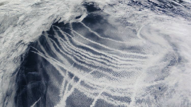
Figure 11 is a satellite view of the northern Pacific Ocean, showing a scene with low
clouds. The white stripes are ships’ tracks, caused by the exhaust from their engines, which
adds additional CCN into the air. The extra CCN change the microphysics of the clouds, with
result that the cloud droplet number density increases (the cloud becomes whiter) and more
sunlight is reflected back to space. Although these ships’ tracks are not caused by cosmic
rays, the image illustrates that any systematic change in CCN will be important for Earth’s
energy budget.
In order to explain how cosmic rays might affect the number of CCN, a mechanism is
required. This is summarised in Figure 12. First, solar variability manifests itself as changes
in the solar wind, which carries the Sun’s magnetic field. The solar wind then modulates
the cosmic ray flux, which is responsible for atmospheric ionisation (producing positive and
negative ions). These charged particles help the formation and stabilisation of new small
aerosols from trace gases in the atmosphere. One of the most important trace gases is sul-
phuric acid, which is produced naturally in the atmosphere by photochemistry.
In 2006, it was shown experimentally that cosmic rays help the initial formation (‘nu-
cleation’) of small aerosols (1–2 nm), and it was found that by increasing the ionisation, the
number density of nucleated aerosols increased as well. 54 These results were later confirmed
by the CLOUD collaboration experiment at CERN in Geneva. 55
For a while, it was thought that the increase in small aerosols (∼3 nm in size) would au-
13Figure 11: Low marine stratus clouds in the northern Pacific Ocean.
Milky Way
Galactic cosmic rays
Reflected
sunlight
Atmospheric
Photochemistry ionisation
H2 O
H2 SO4
1–2 nm 20 nm 50 nm 15μm
Trace gases Ion nucleation Growth by CCN Cloud Cloud
condensation, droplets formation
ion condensation
Figure 12: The physical mechanism linking solar activity variations to climate change.
In summary, the link is: (a) a more active Sun, (b) stronger solar wind, (c) fewer cosmic rays, (d)
less atmospheric ionisation, (e) less nucleation and slower growth, (f ) fewer CCN, (g) clouds
with less droplets, (h) less reflectivity, (i) less reflection of sunlight and a warmer Earth.
14tomatically lead to an increase in the number of CCN (50–100 nm). However, numerical re-
sults from ‘state of the art’ aerosol simulations suggested that this was not the case. 56 Even
large changes in aerosol nucleation (1–2 nm) appeared not to result in an increased num-
ber of CCN. The explanation for this negative result was that additional aerosols would lead
to increased ‘competition’ for the available gases, resulting in slower growth and a larger
probability of a small aerosol becoming incorporated into a larger one before reaching CCN
size.
These numerical results have since been tested experimentally. 57 First the experiment
simulated what would happen in the atmosphere without the presence of ions. Figure 13a
shows how the molecular clusters fail to grow sufficiently to provide significant numbers of
CCN of more than 50 nm in diameter.
1.8
(a) CCN size
1.6
Particle increase
1.4
1.2
1.0
0.8
0 10 20 30 40 50 60 70
1.4
(b) CCN size
Particle increase
1.3
1.2
1.1
1.0
0.9
0.8
0 10 20 30 40 50 60 70
Particle size (nm)
Figure 13: Experimental test of aerosol growth into CCN.
(a) Without ionisation; (b) with ionisation. Adapted from Svensmark (2012). 57
This is what existing theories predict. But when the air in the chamber is exposed to
ionising radiation, so as to simulate the effect of cosmic rays (Figure 13b), the clusters grow
much more quickly to the sizes at which they will help water droplets form and make clouds.
This result contradicts the numerical modelling results, and indicates that an important part
of the ion-mechanism is missing from the theory.
So the evidence is that ions help the growth of aerosols to CCN sizes, but how? The
answer was only found very recently, theoretically and experimentally. The solution is to
include a so-far-ignored contribution to growth of aerosols: from the mass of the ions. Ions
are relatively scarce in the atmosphere, but the electromagnetic interaction between them
and aerosols can compensate for the scarcity and make fusion between ions and aerosols
much more likely. Even at low ionisation levels, about 5% of the growth rate of aerosols is
due to ions. In the case of a near supernova, ionisation can be much greater, and the ion
effect can be responsible for more than 50% of the growth rate. This will have a profound
impact on the clouds and the Earth’s temperature. 58
15These results are also supported by observations. On rare occasions, ‘explosions’ on the
Sun, known as ‘coronal mass ejections’, result in a plasma cloud that passes the Earth, causing
a sudden decrease in the cosmic ray flux that lasts for a week or two. Such events are called
‘Forbush decreases’, and are ideal to test the link between cosmic rays and clouds. Finding
the strongest Forbush decreases and using three independent cloud satellite datasets and
one dataset for aerosols, a clear response in clouds and aerosols to Forbush decreases is seen.
Figure 14 shows the sum of the five strongest Forbush decreases (red curves) together with
various signals observed in clouds (blue curves) in the days around the minimum in cosmic
rays. The difference in the position of minima of the two curves is due to the time it takes
aerosols to grow into cloud condensation nuclei. These results suggest that the whole chain
– from solar activity, to cosmic rays, to aerosols (CCN), to clouds – is active in the Earth’s atmo-
sphere. 59,60 Moreover, they indicate that the cosmic ray–cloud link is capable of explaining
the magnitude of around 1 W/m2 of the observed forcing over the solar cycle.
Aeronet SSM/I MODIS ISCCP
Ångström Cloud water Liquid water Low IR
exponent* content cloud fraction cloud fraction
3.3 5
9.2
Liquid water cloud fraction (×10-1 )
3.6
1.3
Low IR cloud fraction (×10-1 )
0
9.0
CWC (× 10-2 kg/m2 )
AE 340–400 nm
Climax (%)
3.2
-5
8.8 3.5
1.2
-10
8.6
3.1
3.4
-15
1.1 8.4
-10 0 10 20 -10 0 10 20 -10 0 10 20 -10 0 10 20
Days Days Days Days
Extent of Forbush decrease Cloud parameter response
Figure 14: Changes in cloud parameters before and after Forbush decreases.
Changes in daily averages, averaged over the five strongest events between 1990 and 2005. 59
The data shows that reductions in the cosmic ray flux translate into changes in cloud properties.
*The Ångström exponent measures the density of aerosols in the atmosphere.
Changes in the Earth’s electrical circuit
Other ideas have been put forward to explain the Sun–climate link. One idea has to do with
the Earth’s electrical field, which is caused by the potential difference between the iono-
sphere and Earth’s surface. This potential difference is maintained by thunderstorms, and
results in a fair-weather current of atmospheric ions that discharges the potential difference.
The atmospheric ions are mainly produced by cosmic rays, but the electrical circuit is also re-
sponsive to changes in the solar wind. It has been proposed that changes in the electrical
current influences cloud microphysics, for example by affecting the freezing point of cloud
droplets. 61 However, there are a few observations that support an effect of the electric field
16on cloud properties. Harrison and Ambaum 62 studied changes in the atmospheric poten-
tial at a location in the UK and cross-correlated the observations with the downwelling long
wave radiation and diffuse short wave flux. Their data display a two-minute time delay in the
cross-correlations and they suggest that this is evidence of the electric field affecting cloud
properties.
6 Future solar activity
Predicting changes in solar activity is beyond our current capabilities. Even predicting the
size of the next solar cycle is very uncertain. As an example, 105 predictions were made of
the maximum number of sunspots for solar cycle 24 – the current instance of the 11-year
cycle. The predictions were based on either statistical or physical dynamo models, and the
collection of predictions had a form close to a normal distribution, with a mean and variance
of 106 ± 31. 63 However, in the event, the observed maximum of cycle 24 was small: close to
82. This failure epitomises the problems facing those seeking to forecast solar activity.
With a maximum of 82 annually averaged sunspots during solar cycle 24, solar activity is
now the lowest it has been in a century. In contrast, the period 1950–1995 had the highest
solar activity in perhaps 1000 years. This is by no means a surprise, because both sunspots
and cosmogenic isotopes show that solar activity can be highly variable. The interesting
question is how low future solar activity might get. There are already suggestions that solar
activity is moving towards a grand minimum along the lines of the Maunder Minimum, or
perhaps a less severe one, like the Dalton Minimum (see Figure 2). Grand minima are by no
means rare; they have likely occurred 7–9 times over the Holocene period (see, for example,
Figure 7). It is therefore interesting to consider if the Sun is currently moving into a new
grand minimum or just a period of low solar activity, and to think about the consequences
for the Earth’s climate. This depends, of course, on the actual physical mechanisms linking
solar activity to climate.
There have been a number of modelling results aimed at predicting the future effect of
solar activity. If small TSI variation is assumed, the predicted effects will of course be small
and insignificant too. 64 Assuming a 0.25% drop in TSI, the model results indicate a small
drop in projected temperatures in the year 2100: just 0.2–0.3 K. 65,66 However, at least one
projection – based on a simple energy-balance calculation – suggests that the temperature
will drop by a more significant ∼1 K and lead to a new little ice age. This calculation is based
on a large change in TSI of 0.5% 67 (see discussion of TSI variations in Section 2).
The influence of a possible grand minimum has also been studied relative to the IPCC’s
anthropogenic greenhouse gas emission scenarios.
7 Discussion
Based on the numerous studies that demonstrate a close correlation between solar activity
and climate, it seems safe to say that solar activity is important for climate variability (see Sec-
tion 3). In particular, the many studies examining the Holocene period (the last 10,000 years)
demonstrate remarkable agreement between solar variation and climate, as illustrated in
Figures 6 and 7. The main scientific problem today is therefore to quantify and understand
the solar influence on climate.
It should be noted that the observed climate variation on century-to-millennia timescales
is not reflected in atmospheric carbon dioxide levels: according to ice-core data, these have
17been relatively constant. 68 It is therefore unlikely that variations in carbon dioxide concen-
tration have had any influence on the climate variability on these timescales.
Impact of solar activity
Climate models including only small changes in TSI, of the order of 0.1%, suggest that the
solar contribution to climate variation is small, and that anthropogenic greenhouse gases,
aerosols, and volcanoes are the main cause of recent and future climate changes. Some
temperature reconstructions over the last millennium, such as those by Michael Mann and
colleagues, 22,69 and climate model runs for the same period, show little or no trace of the
Little Ice Age (see Figure 5), and are therefore unsurprisingly consistent with a small solar TSI
forcing. However, temperature reconstructions with a small change (0.1–0.2 K) between the
Medieval Warm Period and the Little Ice Age are inconsistent with a large number of other
climate reconstructions. 23,34,41,70–76 For example, temperature reconstructions using bore-
holes are some the most robust paleoclimate indicators available, because they are a direct
physical record of temperature changes occurring at the surface. The study of Huang et al. is
based on hundreds of boreholes from all continents (except Antarctica) and gives strong ev-
idence for a temperature difference of 1.0–1.5 K between the Medieval Warm Period and the
Little Ice Age (see Figure 5). 23 In addition Mann’s temperature reconstructions 22,69 have been
seriously questioned. 77–81 Temperature variations of the order of 1.0–1.5 K between periods
of high and low solar activity, as seen repeatedly over the Holocene period (see Figure 7),
seem much more likely than the limited changes suggested in those studies.
This suggests that either there are larger TSI variations on long timescales and/or that
there is an indirect solar mechanism operating in the atmosphere. The consensus value for
variation in TSI , at around 0.1%, seems small, and, if true, TSI variations cannot explain ob-
served climate changes. 16 In contrast, there are TSI reconstructions that suggest much larger
variations, of the order of 0.4%, which would be important for climate variability. 14,15 As dis-
cussed in Section 2, the basis for thinking there may be such large changes is the possibility
that the irradiance from the quiet Sun varies significantly in time. However, this is at present
a hypothesis with no observational support. It is to be hoped that future observations can
constrain possible TSI variations.
Since solar activity has had a large impact on past climate, it should not be too con-
troversial to assume that the 20th century increase in solar activity must also have had an
influence on the observed temperature increase. If the Sun has had a significant influence
over the 20th century temperature increase, then climate sensitivity has to be on the low
side. Ziskina and Shaviv 82 used a simple model to estimate the relevant forcing over the
20th century, by constraining the fits to the observed temperature, including anthropogenic
(greenhouse gases and aerosols) and a solar contribution. The result is a 20th century so-
lar forcing of 0.8±0.4 W/m2 and a climate sensitivity of 0.25±0.09 K/(Wm-2 ). These numbers
should be compared with the IPCC-estimated radiative forcing on climate from solar activity
between 1750 and 2011 of around 0.05 W/m 2 and a climate sensitivity of 0.9±0.3 K/(Wm-2 ). 1
Therefore, with a larger role for the Sun, the implications on future climate change will be
significant. Such a result should warrant further research into the solar impact on climate.
The situation is better constrained in the modern period – after 1978 – where TSI has
been measured by satellites, giving secure observational evidence for a 0.1% change over
the solar cycle. It is found that the energy that enters the oceans over a solar cycle is 5–7
times larger than the 0.1% change in TSI. 38 This means two things:
18• the solar contribution to the energy that enters the oceans is larger than from TSI alone
by almost an order of magnitude 38,83
• there must be a mechanism capable of amplifying solar activity (see Section 4).
A number of amplifying mechanisms have been suggested.
Solar UV mechanism
One mechanism is based on changes in the UV part of the solar spectrum. During solar max-
ima, the energy in the UV spectrum can be several percent higher than during solar minima.
The increase in UV is absorbed in the stratosphere, which then gets warmer. This results in
changes in the dynamical circulation of the stratosphere, such that energy is transported
down into the troposphere, where it may influence surface temperatures. 43 The UV mecha-
nism has been tested by extensive numerical modelling, 44,45 and it is found that the effect
on the troposphere appears to be too weak to explain the observed changes in the global
radiative budget over the solar cycle. The UV mechanism is the most mature theory put for-
ward to explain solar amplification, in the sense that the physics is understood, and that the
mechanism has been tested in global circulation models.
Cosmic ray clouds mechanism
Another possible mechanism is changes to Earth’s cloud cover due to solar modulation of
cosmic rays. 50–52 In 1996, satellite observations showed that Earth’s cloud cover changed by
around 2%, in phase with changes in cosmic rays, over a solar cycle. Such a variation cor-
responds to a change in radiative forcing of around 1 W/m 2 , which would be in agreement
with the observed changes in energy entering the oceans (see Figure 9). The fundamental
idea is that cosmic ray ionisation in the atmosphere is important for the formation 54,55 and
growth of small aerosols into CCN, which are necessary for the formation of cloud droplets
and thereby clouds. 58 Changing the number density of CCN changes the cloud microphysics,
which in turn changes both the radiative properties and the lifetime of clouds (see Figure 12).
There is now theoretical, experimental and observational evidence to support the cos-
mic ray–cloud link, 57,58 although it should be mentioned that satellite observations of cloud
changes on 11-year timescales are by no means entirely reliable due to inherent calibration
problems. However, in support of the theory, the whole link from solar activity, to cosmic ray
ionisation to aerosols to clouds, has been observed in connection with Forbush decreases
on timescales of a week. 59,60 The cosmic ray variations in response to the stronger Forbush
decreases are of similar size to the variations seen over the 11-year solar cycle and result in
a change in cloud cover of approximately 2%. 60
Cloud variations are one of the most difficult and uncertain features of the climate sys-
tem, and therefore cosmic rays and their effect on clouds will add important new under-
standing of this area. There have been attempts to include the effect of ionisation on the
nucleation of small aerosols in large numerical models, 56,84,85 but important physical pro-
cesses are missing. 58
Although there are uncertainties in all of the above observations, they collectively give
a consistent picture, indicating an effect of ionisation on Earth’s cloud cover, which in turn
19can strongly influence climate and Earth’s temperature. Nonetheless, the idea of a cosmic-
ray link to climate has been questioned, 86–89 and can still give rise to debate. But as more
data from observations and experiments are obtained, the case for the link has only be-
come stronger. For example, if the cosmic ray–climate link is real, then any variation of the
cosmic ray flux, including those which have nothing to do with solar activity, will translate
into changes in the climate as well. Over geological timescales, large variations in the cosmic
ray flux arise from the changing galactic environment around the solar system. A compari-
son between reconstructions of the cosmic ray flux 4 and climate5 over these long timescales
demonstrates that, over the past 500 million years, 6 ice ages have arisen in periods when the
cosmic ray flux was high, as the theory predicts. 90–93 Even the solar system’s movement in
and out of the galactic plane can be observed in the climate record. 94,95
Electric field mechanism
The effects of the electrical circuit on Earth’s climate have also been suggested as a possi-
ble driver of climate. The global atmospheric electrical circuit and its interaction with cloud
microphysics (and hence the cosmic ray effect) is an interesting area of climate science, but
needs observations and experiments to enable an assessment of its importance. 61,96,97
8 Conclusion
Over the last 20 years, much progress has been made in understanding the role of the Sun
in the Earth’s climate. In particular, the frequent changes between states of low and high
solar activity over the last 10,000 years are clearly seen in empirical climate records. Of these
climate changes, the best known are the Medieval Warm Period (950–1250 AD) and the Little
Ice Age (1300–1850 AD), which are associated with a high and low state of solar activity,
respectively. The temperature change between the two periods is of the order of 1.0–1.5 K.
This shows that solar activity has had a large impact on climate. The above statement is
in direct contrast to the IPCC, which estimates the solar forcing over the 20th century as
only 0.05 W/m2 , which is too small to have a climatic effect. One is therefore left with the
conundrum of not having an explanation for the difference in climate between the Medieval
Warm Period and Little Ice Age. But this result is obtained by restricting solar activity to only
minute changes in total solar irradiance.
There are other mechanisms by which solar activity can influence climate. One mecha-
nism is based on changes in solar UV radiation. However, the conclusion seems to be that the
effect of UV changes is too weak to explain the energy that enters the oceans over the solar
cycle. In contrast, the amplification of solar activity by cosmic ray ionisation affecting cloud
cover has the potential to explain the observed changes. This mechanism is now supported
by theory, experiment, and observations. Sudden changes in cosmic ray flux in connection
with Forbush decreases allow us to see the changes in each stage along the chain of the
theory: from solar activity, to ionisation changes, to aerosols, and then to cloud changes.
In addition, the impact of cosmic rays on the radiative budget is found to be an order
of magnitude larger than the TSI changes. Additional support for a cosmic ray–climate con-
nection is the remarkable agreement that is seen on timescales of millions and even billions
of years, during which the cosmic ray flux is governed by changes in the stellar environment
of the solar system; in other words, it is independent of solar activity. This leads to the con-
clusion that a microphysical mechanism involving cosmic rays and clouds is operating in the
20Earth’s atmosphere, and that this mechanism has the potential to explain a significant part
of the observed climate variability in relation to solar activity.
An open question is how large secular changes in total solar irradiance can be. Current
estimates range from 0.1% to outlier estimates of 0.5%; the latter would be important for
climate variation. A small TSI variation, on the other hand, would mean that TSI is not re-
sponsible for climate variability. Perhaps future observations will be able to constrain TSI
variability better.
Climate science in general is, at present, highly politicised, with many special interests
involved. It should therefore be no surprise that the above conclusion on the role of the Sun
in climate is strongly disputed. The core problem is that if the Sun has had a large influence
over the Holocene period, then it should also have had a significant influence in the 20th
century warming, with the consequence that the climate sensitivity to carbon dioxide would
be on the low side. The observed decline in solar activity would then also be responsible for
the observed slowing of warming in recent years.
Needless to say, more research into the physical mechanisms linking solar activity to cli-
mate is needed. It is useless to pretend that the problem of solar influence has been solved.
The single largest uncertainty in determining the climate sensitivity to either natural or an-
thropogenic changes is the effect of clouds, and research into the solar effect on climate will
add significantly to understanding in this area. Such efforts are only possible by acknowl-
edging that this is a genuine and important scientific problem and by allocating sufficient
research funds to its investigation.
219 Appendix: A simple ocean model calculation
The following simple calculation illustrates why variations in TSI are too small to explain the
observed variations in ocean temperature over the 11-year cycle. For a more comprehensive
treatment, see Shaviv (2008). 38
The solar constant at the top of the Earth’s atmosphere is measured at:
S0 = 1365 W/m2 (1)
This energy needs to be distributed over the Earth’s surface
πr 2 S0
S = S0 2
(1 − α) = 0.7 ≈ 239 W/m2 (2)
4πr 4
where α ≈ 0.3 is the Earth’s average albedo from ice, clouds, land and ocean. Over a solar
cycle the irradiance from the Sun changes by ≈0.1%, corresponding to 1.4 W/m2 . Using the
same arguments as above, the change at the surface becomes:
ΔS0
ΔS = 0.7 ≈ 0.24 W/m2 (3)
4
This is the change from peak to peak. The amplitude over a solar cycle is then
ΔSA ≈ 0.1 W/m2 (4)
So now we have the change in energy that on average goes into the ocean during a
solar cycle due to solar irradiance changes. We will now use a simple model 83 to estimate
the expected temperature change ΔT caused by a periodic solar irradiance signal over the
11-year period:
dΔT ΔSA
+ K ΔT = cos(ωt) (5)
dt ρ H CP
where ΔT is the change in temperature, K is a dissipative timescale for energy loss to the
deep ocean and to the atmosphere. H is the average depth of the mixed layer of the oceans
and Cp is the heat capacity of water at constant pressure, and finally ρ is the density of wa-
ter (see Figure 15. The assumption is that in the mixed layer the water is well mixed and
therefore the temperature can be described by a single number ΔT .
Solving the above equation by Fourier transformation gives (inserting, ΔT = ΔTω exp(iω)):
ΔSA
ΔT = cos(ωt + θ) (6)
ρ H CP (ω 2 + K 2 ) 1/2
The above equation also gives the amplitude in the temperature response to a solar-cycle
variation in irradiance, and the phase shift θ is related to the dissipative scale K and ω via
tan θ = ω/K (7)
Observing the phase shift can therefore give us the dissipative scale K. The relevant con-
stants are:
K = 1 year−1 = 3.1 ∙ 10−8 s−1 (8)
H = 50 m
CP = 4.2 ∙ 103 WsK−1 /kg
ρ = 1.0 ∙ 103 kg/m3
ω = 2π/11.0 years−1 = 1.8 ∙ 10−8 s−1
22You can also read