Forecasting Extreme Volatility of FTSE-100 With Model Free VFTSE, Carr-Wu and Generalized Extreme Value (GEV) Option Implied Volatility Indices
←
→
Page content transcription
If your browser does not render page correctly, please read the page content below
1

     Forecasting Extreme Volatility of FTSE-100 With Model Free
    VFTSE, Carr-Wu and Generalized Extreme Value (GEV) Option
                      Implied Volatility Indices

                      Sheri M. Markose1, Yue Peng* and Amadeo Alentorn*†

Abstract
Since its introduction in 2003, volatility indices such as the VIX based on the model-free
implied volatility (MFIV) have become the industry standard for assessing equity market
volatility. MFIV suffers from estimation bias which typically underestimates volatility
during extreme market conditions due to sparse data for options traded at very high or
very low strike prices, Jiang and Tian (2007). To address this problem, we propose
modifications to the CBOE MFIV using Carr and Wu (2009) moneyness based
interpolations and extrapolations of implied volatilities and so called GEV-IV derived
from the Generalised Extreme Value (GEV) option pricing model of Markose and
Alentorn (2011). GEV-IV gives the best forecasting performance when compared to the
model-free VFTSE, Black-Scholes IV and the Carr-Wu case, for realised volatility of the
FTSE-100, both during normal and extreme market conditions in 2008 when realised
volatility peaked at 80%. The success of GEV-IV comes from the explicit modelling of
the implied tail shape parameter and the time scaling of volatility in the risk neutral
density which can rapidly and flexibly reflect extreme market sentiments present in
traded option prices.

Keywords: Extreme Events;VFTSE; Model-Free Implied Volatility; Generalized
Extreme Value; Implied Tail Index; Volatility Forecasting

JEL Classifications: C13, C16, G01

1
 Sheri Markose is the corresponding author, Professor, Economics Department University of Essex,
Wivenhoe Park , Colchester CO3 4SQ, Essex, UK, scher@essex.ac.uk.
*Centre for Computational Finance and Economic Agents, University of Essex, UK
†Old Mutual Asset Management (OMAM), UK.
The authors are grateful for discussions with Stephen Figlewski, Thomas Lux, David Veredas, Radu Tanaru,
George Skiadopoulos and John O‟Hara. We remain responsible for errors and omissions.
2

1. Introduction
The recent financial crisis which started in 2007 has resulted in periods of extreme
volatility in financial markets. This has prompted new studies on the behaviour of stock
market volatility (see, Schwert, 2011, Mencía and Sentana, 2011, Andersen et. al. 2011
and Bollerslev and Todorov, 2011), especially in conjunction with option price implied
volatility indexes such as the VIX.         Since the introduction in 1993 by the Chicago Board
of Trade (CBOE) of the equity market volatility index2 based on the seminal work of
Whaley (1993) on the implied volatility obtained from both call and put equity index
options, the information content of the volatility index in forecasting future realized
volatility has become an area of intense investigation.             Whaley (2000) coined the term
“investor fear gauge” to highlight the fact that the volatility index peaks when the
underlying market index is at the lowest level and hence reflects investors‟ fear about
market crashes. The volatility index also features in the pricing of volatility derivatives
for hedging non-diversifiable market risk and is also cited in the management of systemic
risk conditions.

In September 2003, the CBOE adopted the so called model-free method, for the
construction of the VIX.           Technically, VIX is the square root of the risk neutral
expectation under a Q-measure of the integrated variance of the SP-500 over the next 30
calendar days reported on an annualized basis. The replication of this is independent of
any model and involves only directly observed prices for out-of-the-money calls and
out-of-the-money puts with the same maturity (see, Britten-Jones and Neuberger, 2000
and Carr and Madan,1998). 3 The relationship between the implied volatility and
historically realized volatility has particular significance as the measure of volatility risk
premium.      As risk averse investors buy index options to hedge their underlying equity
positions, Carr and Wu (2009), Bollerslev, Tauchen and Zhou (2009) and others have

2
  The original CBOE volatility index, now referred to as VXO, was based on at the money Black-Scholes
(1973) implied volatility. VXO is based on the SP-100 returns while the revamped VIX of 2003 has the
SP-500 as the underlying.
3
  Carr and Madan (1998) refined the model-free framework for option implied variance in the context of
determining the variance swap rates. The VIX and volatility indexes adopted by the various exchanges for
their stock indexes (such as VFTSE, VDAX, VX1 and VX6) are estimated as the square root of the model
free implied variance. The Demeterfi et. al.(1999) fair value of future variance method has been shown by
Jiang and Tian (2007) to be identical to the model free implied variance.
3

found that typically the spot VIX computed from option prices embeds volatility risk
premium and exceeds expected realized volatility obtained under the P-measure.
During turbulent market conditions, the value of traded option based volatility index goes
up. However, the lack of robustness in the MFIV method for the VIX first identified by
Jiang and Tian (2007), expecially under extreme market conditions, has implications for
mispricing volatility derivatives such as VIX futures, options and variance swaps.
Mencía and Sentana (2011) investigate the mispricing of volatility derivatives during the
recent crisis.   There is a large and growing literature on information from traded option
implied distribution volatility indexes for their capacity (see, Giamouridis and
Skiadopoulos, 2010, for a recent survey) to forecast future realized volatility and other
statistics on the underlying asset. In recent conditions of severe market distress,
Andersen et. al. (2011) have noted discrepancies in the intraday VIX in not showing a
consistent inverse relationship with the underlying stock index, a condition that the „fear
guage‟ should satisfy especially during turbulent market conditions.

The objective of this paper is to use the extreme market volatility of about 30%-80%
recorded in all the major stock index (daily) returns during the recent subprime financial
crisis from mid 2007 to mid 2009 to test out the efficacy of differently constructed IV
indexes to forecast realized volatility both in so called normal market conditions when
volatility is no more than about 20% and during extreme market conditions.     For this we
analyse data on the FTSE-100 and its model free VFTSE volatility index from January
2000 to June 2009.     The paper aims to test the MFIV using the VFTSE and to propose
alternative IV models that can specifically deal with the interspersed nature of relatively
calm periods with periods of extreme volatility of stock index returns.   In particular, we
aim to show how the implied volatility analytically derived from a closed form option
pricing result of Markose and Alentorn (2011) using the Generalized Extreme Value risk
neutral density (GEV-RND) can overcome the well known problems of MFIV and other
extant methods of dealing with time varying tail shape of RND and resulting normal and
extreme implied volatilities.   The issues involved here are briefly reviewed below.
4

Figure 1: FTSE 100 index level and FTSE-100 volatility index, VFTSE (January
2000-June 2009) Right hand side axis the VFTSE levels and the Left Hand side Axis the
FTSE-100 levels

Figure 1 plots the FTSE 100 index level (blue) and its volatility index, VFTSE (green),
from 4th January 2000 to 1st June 2009.    It shows that in relatively calm periods, the
VFTSE volatility index ranges between 10% to about 20%. However, there are also
some spikes in the VFTSE series.     On 11th September 2001 (9/11), VFTSE spiked at
around 50%, and during the American invasion of Iraq in March 2003, VFTSE peaked at
over 40%. The spike points of VFTSE during the crisis of autumn 2008 have been
much higher than any recent market down turn.      The recent crisis has manifested in
extreme spikes in VFTSE at about 55% on the 15th September 2008 corresponding to
Lehman Brother Bankruptcy and near 80% on the 28th October 2008.         At about the
latter spike of the VFTSE, the FTSE-100 records the first of its extreme minima followed
by its all time low of this period in early March 2009.

Engle (2010) has stated that “this crisis involved 99% confidence set of events”.
5

Model-free and non-parametric methods, in general, for option price implied statistics
which rely on sparse data for options traded at very high or very low strike prices may
not be able to capture extreme tail behaviour around the 99% confidence level of the
underlying returns data.          Hence, parametric models become unavoidable, replacing
sampling error with model error, Markose and Alentorn (2011).                        The CBOE MFIV
which has increasingly become industry standard globally has been called into question
by Jiang and Tian (2007).         They identify so called truncation and discretization errors in
the CBOE procedure. Truncation errors arise from ignoring strike prices beyond the
range of listed strike prices and discretization errors are ascribed to an ad hoc numerical
integration scheme to fill in discrete data points for the strike prices.                Using simulated
option price data for listed strike prices on a typical trading day Jiang and Tian (2007)
show that the CBOE model-free method for the VIX can lead to an underestimation of
the true volatility by about 198 basis points and overestimation by 79 basis points.4 The
worrisome point is that when the true volatility is high, the truncation errors kick in with
large undestimation of implied volatility by the CBOE method.                  The fact that inadequate
asset pricing models that failed to capture extreme market price drops contributed to
chronic underpricing of credit risk and market risk that characterized the lead up to the
recent financial crisis failure should add to the urgency of the Jiang and Tian (2007)
agenda to improve accuracy of risk neutral pricing models for volatility.

Andersen and Bondarenko (2007) have aptly identified VIX and other MFIV as corridor
implied volatility (CIV) measures with barriers set at the lowest (Kl) and the highest (KH)
strikes being used on a given day to compute the index.               Andersen et. al. (2011) note
that there is a lack of coherence in the VIX method on how return variation over the tail
areas ([0; Kl] and [KH;∞]) is accounted for at different points in time.5 Andersen et. al.
(2011) specify the use of a ratio statistic which indicates how far into the tail a given
strike price K is and they propose a „coherent‟ method for the selection of truncation
strikes which is defined as the inverse function of a fixed percentile (typically [0.01, 0.99]

4
  Jiang and Tian (2007) state that these translate to dollar values that range between - $1,980 and +£790 per
contract.
5
  The well known way of dealing with this is to take an effective range of moneyness with the highest and
lowest strikes given as a ratio of at- the- money Black-Scholes implied volatilities, Figlewski (2002).
6

or [0.03,0.97]) of the ratio statistic. Recently, Extreme Value Theory (EVT) is being used to
model the return variation in the tail areas under a Q risk neutral measure.   In order to
overcome ad hoc truncations and/or extrapolations into the tails of the option price
implied risk neutral density (RND), Figelwski (2010) gives a parametric solution to an
otherwise non-parametric model for the rest of the RND by using the Generalized
Extreme Value (GEV) distribution for the tails of the RND.           Bollerslev and Todarov
(2011) specify a semi-parametric Lévy density function based on the Generalized Pareto
Distribution to model the left and right tails of the returns distribution under both Q and P
measures in the context of capturing extreme movements in the variance risk premium. In
Bollerslev and Todarov (2011) the generalized method of moments is used to estimate
the Q tail parameters from observed option prices with the log moneyness set at 0.9 and
1.1 for the left and right tails, respectively.

In this paper, in order to solve the problems encountered in the CBOE MFIV, we specify
two methods.      In the first method we modify the CBOE MFIV by following the steps
taken by Carr and Wu (2009) (hence CW-IV) in the discretization needed for
synthesizing the variance swap rate, based on interpolation and extrapolation in the
implied volatilities at different moneyness levels of the options.        We use the cubic spline
interpolation recommended by Jiang and Tian (2007) and retain a fixed 8 times average
implied volatility extrapolation scheme from Carr-Wu (2009). These adjustments can
improve the accuracy of the IV calculation, especially in combating the problem of sparse
data points at extreme tail regions.       However, the limitation of this method is that it
requires a pricing model such as Black (1976) to derive the implied volatilities for
interpolation and extrapolation.       This makes the approach no longer 'model-free' and
runs the risk of model error.       Further, there are issues relating to the construction of
fixed 30 day horizon IV which follows the CBOE MFIV method of using options of only
two maturities.    The linear interpolation of the IVs of the closest and the second closest
to maturity options that include the 30 day horizon assumes a linear term structure for
implied variance in option maturity. Also there are roll over effects on IVs when near
(and second) maturity month options are switched at about 7 days to maturity.
7

The second IV model we consider is based on the recently developed Markose and
Alentorn (2011) closed form solution for option pricing using the Generalised Extreme
Value (GEV) distribution for the risk neutral density.     It is a parametric model which
relies on the scale and tail shape parameters of the GEV distribution.    Depending on the
tail shape parameter which also controls the size and skew of the tails of the distribution,
the GEV distribution subsumes the three classes of distributions.      A zero value for the
tail shape parameter yields the Gumbel class (which includes the normal, exponential and
lognormal distributions) which have zero skew in the probability mass and symmetry in
right and left tails.   Positive value for the tail shape parameter yields the so called
Fréchet class that is able to capture the fat tailed behaviour with the maxima of a
stochastic variable.    Negative value for the tail shape parameter yields the “reverse”
Weibull class of distribution for the corresponding minima of the stochastic variable.
Larger the non-zero values for the tail shape parameter lead to increased higher moments
including the variance, skewness and kurtosis of the GEV distribution.      As the selection
of the tail shape parameter is not restricted apriori but is backed out from the traded
option price data, the GEV model mitigates model error.

Markose and Alentorn (2011) find that GEV-RND yields results that strongly challenge
traditionally held views on tail behaviour of asset returns based on Gaussian distributions
which predicate simultaneous existence of thin tails in both directions during all market
conditions. The GEV RND which is governed by the option price implied tail shape
parameter is found to switch tail shape with underlying market conditions. A non-zero
value for the tail shape parameter results in significant skewness in the probability mass of
the GEV density function during extreme market conditions which implies large one
directional movements and truncation in the probability mass in the other direction.
During extreme market turbulence, a positive value for the tail shape parameter of the GEV
RND function for losses implies extreme price drops, while a large negative tail shape
value signal large price increases. These switches in the implied tail shape parameter
result in a much larger GEV-IV than can be obtained by other parametric and
non-parametric methods during turbulent market conditions. Likewise, during normal
market conditions, a close to zero or negative tail shape around -.3 for the GEV-RND
8

implies a much smaller GEV-IV than what is obtained by most other methods. To date,
proposed option pricing models intended to deal with extreme and asymmetric volatility,
fat tails and the skew in asset returns have failed to highlight the above characteristic
features of the GEV-RND.6 Thus, as first demonstrated in Markose and Alentorn (2011),
GEV-RND can capture both market perceptions of fat tailed behaviour, as well as,
expectation of calmer periods consistent with the Gumbel class of distributions.
Remarkably, this is achieved with none of the truncation and extrapolation exercises to
capture extreme implied volatility that is encountered in model-free methods.

Markose and Alentorn (2008) also find that the GEV RND yields better estimates for high
quantile extreme Value-at-Risk for a 10 day constant horizon than a number of parametric
and non-parametric methods for this. The success in overcoming option maturity effects
in order to report constant horizon implied GEV-RND, its quantile and other implied
statistics such as volatility on a daily (or an intra daily) basis comes from using all
maturities for traded options and explicitly backing out the term structure parameter to
scale GEV volatility, Alentorn and Markose (2006). We will adopt this method to address
problems of roll over effects of close to maturity option contracts and of assuming a linear
scaling of the implied variance with time.

The suitably refurbished Carr and Wu (2009) modification for the CBOE method,
CW-IV, the GEV-IV and the Black-Scholes IV (BS-IV) are constructed for a 30-day
fixed horizon based on traded option price data on the FTSE-100.                    For realised volatility
of the FTSE-100, we use the square root of the annualised 30 day daily squared returns
(see, Siriopoulos and Fassas, 2008). We find that the volatility indices from the GEV
model and the Carr-Wu method perform better than the Euronext VFTSE and the BS-IV
for forecasting realised volatility, especially during the recent financial crisis of
2007-2008.       Though we primarily investigate the forecasting performance of the

6
  Other parametric option pricing models that aim to capture leptokurtosis, left skew and extreme volatility
often start with specific fat tailed distributions for the RND such as skewed Student –t distribution, de Jong
and Huisman (2000), or Weibull distribution, Savickas (2002) and hence run into model error. They also
fail to have closed form solutions or end up over-fitting with far too many parameters. For example, the
latter case is the mixture of two log-normals which has to estimate five parameters, Gemill and Saflekos
(2000).
9

different IV models, the benchmark case of lagged realized volatility is also given.
When the data is broken down into subsamples of normal and extreme market conditions,
the GEV-IV yields the best forecast performance, in all cases, followed by the CW-IV.
The GEV-IV performs best due to its explicit reliance on the implied tail shape parameter
and implied volatility term structure parameter which can rapidly and flexibly reflect
extreme and normal market sentiments being impounded in traded options.

The rest of this paper is organised as follows.     Section 2 provides a literature review on
forecasting future realised volatility with implied and historical volatility measures.
Sections 3 and 4 introduce the two different methodologies (Carr-Wu and GEV) for the
construction of the implied volatility index.      Section 5 estimates the realized volatility
and discusses the empirical results on the forecasting comparisons for VFTSE, Carr-Wu
IV, BSIV and past realized volatility, RV. Both univariate and encompassing regressions
are used to test the informational content of the IV and past RV models.         Section 6 gives
concluding remarks.

2. Review of Forecasting Future Realised Volatility with Implied Volatility
Discussions on traded option implied volatility and its efficacy in forecasting realized
volatility has dominated the literature by far (see, Poon and Granger, 2003) though the
role of option implied statistics for their capacity to incorporate market information is
growing (see, Giamouridis and Skiadopoulis, 2010).         The other main contender for
volatility forecasting are times series based historical volatility, HV, models.
Empirically, a regression setting is used to test whether the IV or HV measures are an
unbiased and information efficient forecast of future realized volatility. Unbiasedness is
typically assessed by examining the regression coefficients (intercept=0 and slope=1) of a
univariate regression equation.    Using encompassing regression equations, a forecast
based on IV or HV measure is defined to be information efficient if it is not subsumed by
other forecast variables.   In all cases, efficiency of forecasts requires residual forecast
errors to be white noise.   Although the conclusions are somewhat contradictory and
varied, most authors contend that option implied volatilities provide biased, but more
efficient, forecasts of future volatility than historical volatility measures.   Within the
10

class of IV measures, while Jiang and Tian (2005) found the CBOE MFIV forecasts
better than model based IV such as BS-IV, more recent papers find that modified model
based IV measures including the Black (1976) IV model and the new Corridor Implied
Volatility of Andersen and Bonderanko (2007) can out-perform MFIV constructed by the
different authors and also the industry standard ones such as VIX.

Some of the early papers in this area find that the implied volatility is poor at forecasting
future realised volatility (see, Canina and Figlewski (1993) and Lamoureux and Lastrapes
(1993)). However, Christensen and Prabhala (1998) have countered their results by
stating that the early studies are hampered by poor or insufficient data sets and lack a
proper method for measuring realized volatility. They proceed to use non-overlapping
data and a longer time series and show that the implied volatility outperforms historical
time series based realised volatility such as ARCH and GARCH in forecasting future
realised volatility.

Fleming, Ostdiek, and Whaley (1995) show that the VXO is strongly related to its future
realised volatility and it forecasts realised volatility better than a first order autoregressive
volatility model. However, the forecast result of the VXO has an upward bias. Blair,
Poon, and Taylor (2001) show that the VXO provides almost all relevant information for
forecasting index volatility from one to twenty days.         Additionally, they find that the
VXO gives more accurate forecast results compared with volatility constructed by Risk
Metrics and GARCH type models.           Giot (2003) investigates forecasting volatility and
market risk with the VIX and VXN.          The findings show that the volatility index has a
higher information content than Risk Metrics and GARCH models at different time
horizons.

There are also similar results for forecasting the future realised volatility with the
volatility indices for stock markets in countries other than the US.     For example, Franck,
Patrick, and Christophe (1999) study the Marché des Options Négociables de Paris
(MONEP) Market Volatility Index (VX1) and show that the VX1 is highly related with
realised volatility and performs well in predicting future realised volatility with different
11

time horizons.     The study by Siriopoulos and Fassas (2008) on the FTSE-100
volatility index VFTSE uses the same underlying as we do. They show that the VFTSE
is a biased estimate of future realised volatility but that it includes more information on
future realised volatility than historical volatility based methods.

There are also some opinions contrary to the above.       Areal (2008) shows that the high
frequency data based volatility of the FTSE-100 index gives a better forecast for the
future realized volatility than the implied volatility indices constructed by the author.
The latter were found to contain information on future volatility but they yield biased
measures of future volatility.     Becker, Clements, and White (2007) and Becker and
Clements (2008) show that the model free VIX cannot offer additional information on
volatility forecasts of the S&P 500 market compared with a combination of historical
model based forecasts.       However, no single historical model based forecasts is
necessarily better than the VIX.

When looking exclusively at the forecasting performance of MFIV, the first study of this
is that of Jiang and Tian (2005) on the SP-500 for the period 1988-1994.       They find that
the volatility forecast using MFIV outperforms both BS-IV and past RV.          In the case of
the MFIV constructed by the authors Cheng and Fung (2012) for the Hang Seng Index,
they find that both the MFIV and the futures prices based Black (1976) IV outperform a
number of time series based historical volatility (TS-HV) models in terms of their
forecast power of realized volatility.    Cheng and Fung (2012) find that futures prices
based Black-IV subsumes the information content of both MFIV and TS-HV. Andersen
and Bondarenko (2007) find similar results to Cheng and Fung (2012) that futures prices
based Black-IV dominates MFIV and the VIX while their new Corridor Implied
Volatiltiy subsumes all others.      However, as we discussed in the introduction, the
robustness of the widely used industry standard MFIV is itself in question especially as
the method exhibits truncation errors which leads to an underestimation of volatilty
during market downturns, Jiang and Tian (2007), the focus of this paper is to contrast IV
models that are specifically built to address this and those that are not.   In the following,
we introduce two alternative methods to construct implied volatility indices that can deal
12

with extreme market conditions to see if they can improve on the model free method.

3. Carr-Wu Implied Volatitily With Spline Interpolation and Linear Extrapolation
As we intend to use the Carr-Wu (2009) discretization and truncation scheme to
overcome problems in the CBOE MFIV, we will first briefly outline the CBOE
construction.         The generalized formula (see, CBOE VIX White Paper, 2003) used for
the CBOE implied variance is:

                                                                          2
                  2    2e rT        Ki             1 F
                                     2
                                       Q(T , K i )                    1 .         (1)
                        T      i   Ki              T K0

Here T is the time to maturity of the index option, r is the risk-free interest rate, F is the is
the maturity matched forward index level, K0 is the first strike below F (K0 ≤ F), Q(T,Ki )
is the midpoint of the bid-ask spread for the call and put options with strike price Ki
where out-of-the-money call options are used if Ki > K0, out-of-the money puts are used
if Ki < K0 and both calls and puts are used for Ki=K0.                              Note,     K i is the strike

increment calculated as
                                                    Ki   1       Ki   1
                                             Ki                               .
                                                             2
At the lowest or the highest strike prices, the strike price increment is simply the
difference between the two two lowest and highest strike prices, respectively. The
put-call parity condition is used to get the maturity matched forward index level at closest
and second closest maturity dates

                                                                                        (2)

Here           is the strike price for which the call option price has the smallest difference

with the put option price and                            are the call (put) option prices at               .7

The second term in (1) implements a correction for the discrepancy betweeen the forward

7
    Closest to maturity options must have at least one week to expiration.
13
price and K0. To obtain a fixed 30 day horizon MFIV, the implied variance in (1) is
evaluated at closest maturitiy date if this is greater than 30 days. If there are fewer than
30 days and next-term options have more than 30 days to expiration, the resulting MFIV
reflects an interpolation of the implied variance in (1) for , viz. and .
This will be defined in (8). Clearly, as the MFIV on the FTSE-100 is readily available
in the form of VFTSE, we use this directly.
However, there are further procedures in the CBOE VIX White Paper (page 6) in the
selection of the calls and puts with respect to the strike prices needed for equation (1)
which we give below having fully expanded Q(T , K i ) 8:
rT j rT j
2 2e Ki C 2e Ki P
j (K i ) (K i )
Tj Ki K0 K i2 Tj
Tj Ki K0 K i2 Tj
2
(3)
2 K 0 rT j C 2 K 0 rT j P 1 F
e (K 0 ) e (K 0 ) 1 .
T j K 02 Tj
T j K 02 Tj
Tj K0
We now apply the steps used by Carr-Wu (2009) to address the discretization and
truncation problems in (3). For this, first we take both in-the-money and
out-of-the-money option prices and then estimate the implied volatility with all
available option prices corresponding to the strike prices Ki using the Black
(1976) futures option pricing model expressed in moneyness levels:
C ki
Tj
(k i ) F ( N ( d1 ( k i ) e N (d 2 (k i ))) , (4.a)
P ki
Tj
(k i ) F ( N ( d1 ( k i ) e N ( d 2 (k i ))) (4.b)
8
This can be found at www.cboe.com/micro/vix/vixwhite.pdf. The bids of all the option prices must be
non-zero. The CBOE method first sorts the call options with their strike prices ranked from low to high.
Then it selects call options with strike prices greater than the at- the- money- strike price, A similar
method applies when selecting put option prices. Finally, at both call and puts are selected. The
truncation of out- of- the- money put prices take the following form : if two puts with consecutive prices
with zero bid prices are found then no puts with lower strikes are considered. Likewise for out- of- the-
money calls, once two consecutive call options with zero bid prices are found, no calls with higher strikes
are considered.14
2
ln k i Tj / 2
Here d1 (k i ) and d 2 (k i ) d1 ( k i ) Tj .
Tj
The moneyness level with all available strike prices and the futures price is
defined as
(5)
For each moneyness level , there is a corresponding Black (1976) implied volatility
. Based on the moneyness level from low to high, we can use interpolation to
generate very fine grids. We define the upper and lower bounds of the moneyness level
grids as
(6.a)
and
(6.b)
where , # denotes the average of all available implied volatilities for options with the
respective selected maturities, denotes the generated artificial grids, and .
The maximum and minimum available moneyness levels are denoted as and
.9 Clearly extrapolations into the tails using (+/-)8 times Black (1979) average
implied volatilities # in (6a,b) will reflect the market information for the time varying
nature of the statistic on a daily basis and counter some of the criticism directed at the
lack of „coherence‟ that comes from the CBOE method (see, footnote 8) of moving into
deep OTM tail regions. Andersen and Bondarenko (2011) state that OTM options that
are excluded after two consecutive zero bid quotes are encountered “induces
randomness” in the effective strike range.
We apply a cubic spline interpolation instead of linear interpolation used in Carr and Wu
(2009) to calculate the implied varaince for each corresponding moneyness level
9
Carr and Wu (2009) use 8 times the average implied volatility to make sure the strike price range is big
enough. We also find 8 is a proper magnitude.15
between and .10 For the moneyness level outside and , we apply
a flat extrapolation using the range in (6a,b). For all moneyness levels lower than ,
we use the implied volatility of . Likewise, for all moneyness levels higher than
, we use the implied volatility of . With this interpolation and extrapolation
method we can have implied volatilities which cover a wide range and also have small
strike price intervals and hence achieve a more precise approximation result for the
CBOE replication equation (1). On substituting (4.a.b) into (3) and using (5) and (6a,b)
we have the annualised implied variance, with time to maturity from to :
(7)
Here
and denotes the moneyness level corresponding to at- the- money- strike price, .
In order to calculate the 30-day implied volatility, we follow the CBOE method of
interpolating the implied variance from the two closest maturities. If the closest
maturity, T1, is equal to or greater than 30 calendar days, , then we use the
closest implied variance to the 30 calendar day implied variance of market. If
and , then a linear interpolation between these two is taken. The annualised
30-day implied volatility is the square root of the Carr-Wu implied variance in (7) :
10
The spline interpolation is also recommended by Jiang and Tian (2007) in order to avoid arbitrage
opportunities.16
(8)
4. Implied Volatility with Generalised Extreme Value (GEV) Option Pricing Model
In this section we will derive an implied volatility index that is based on the GEV option
pricing model which can respond flexibly to both extreme market as well as normal
market conditions, Markose and Alentorn (2011). The GEV option pricing model offers a
more accurate and empirically grounded approach to price derivatives, hedge volatility
and estimate value at risk (VaR) under real world conditions as the log-normal
distribution of returns on underlying financial assets has been found not to hold. The
returns on financial assets are found to have fat-tails, skewness and other stylised facts
regarding time varying volatility. Compared with BS model and other parametric models
which make restrictive distributional assumptions, the GEV-RND function can capture
the stylised facts on the non-normal skewness and kurtosis without any apriori
restrictions on the class of distribution being implied for the underlying. Also using the
Alentorn and Markose (2006) method described below, we estimate the constant horizon
30-day implied volatilities of the FTSE 100 from the implied RND term structure of the
GEV model using both put and call options of all maturities on a daily basis. With an
empirically obtained time varying term structure parameter in traded option maturity for
the GEV RND, this model can capture the implied volatility for any time horizon without
assuming the square root law where volatility scales with the square root of time.
4.1 GEV- RND and Option Pricing Model
Following the Harrison and Pliska (1981) arbitrage free option pricing result, under a risk
neutral measure, Q, the call option at current time and with maturity time can be
priced using a risk neutral density (RND) function :
C r (T t )
t ,T (K ) e EtQ [max( S T K ,0)] e r (T t )
(ST K ) g ( S T )dS T (9)
K
The corresponding put option pricing function is given as:17
P K
r (T t )
t ,T (K ) e EtQ [max( S T K ,0)] e r (T t )
(K S T ) g ( S T )dS T (10)
0
Here, EtQ refers to the expectations operator under the risk neutral Q measure. In an
arbitrage-free economy, the following martingale condition must also be satisfied:
r (T t )
St e EtQ ( S T ) . (11.a)
Using the price of index futures, Ft ,T , which expire at the same date as the option, this
condition yields
Ft ,T EtQ ( ST ) . (11.b)
In keeping with the extreme value distribution modelling of economic losses 11, we
assume negative returns defined as follows the GEV density
function for the tail shape parameter 0 (see, Reiss and Thomas, 2001, p.
16-17):
1 1/ 1/
1 ( LT ) ( LT )
f ( LT ) 1 exp 1 (12)
Note, the relationship between the density function for LT and the RND function g(ST) for
the underlying price ST is given by the general formula (see, Baz and Chacko, 2004)
This yields the GEV RND function :
1 1/ 1/
1 ( LT ) ( LT )
g (ST ) 1 exp 1 (13.a)
St
ST
With 1 ( LT ) 1 1 0 for 0. (13.b)
St
11
Since extreme economic losses are more probable than extreme economic gains, the fat tailed or Fréchet
distribution is used to model extreme losses. To this end, we follow the practice of the insurance industry,
Dowd [2002, p 272], and model returns as negative returns. This has also been discussed in Figlewski (2010).18
Here, is location and is the scale parameter of the GEV distribution. Further, is
the tail shape parameter which governs whether the GEV distribution belongs to the
Frechet ( > 0) class or the reverse Weibull class ( < 0). As discussed at length in
Markose and Alentorn (2011), the implied GEV tail shaped parameter changes with
market conditions. In distributions for which ≠ 0, the condition in equation (13.b)
imposes a truncation on the probability mass and a distinct asymmetry in the right and
left tails such that when the probability mass is high at one tail signifying non-negligible
probability of an extreme event in that direction, there is an absolute maxima (or minima)
in the other direction beyond which values of ST have zero probability.12 Only the case
where the tail shape parameter =0 yields thin tailed distributions belonging to the
-1
Gumbel class with the tail index α= being equal to infinity, implying that all moments
of the distribution are either finite or zero. The Gumbel class has zero skew in the
probability mass and displays symmetry in the right and left tails and there is no
condition truncating the distribution in either direction for values of ST.
On substituting (13.a) into (9) and using the constraint in (13.b) to get the upper limit of
integration for the option price, a change of variable operation for the integration enables
Markose and Alentorn (2011) to obtain a closed form solution for a GEV RND based
option price using incomplete and generalized incomplete Gamma functions. Omitting
the proof which can be found in Markose and Alentorn(2011), the GEV- RND call option
price is given as
C r (T t ) H 1/
1/ H 1/
t ,T (K ) e S t (1 )e (1 ,H ) Ke (14)
12
As shown in Reiss and Thomas (2001), kurtosis of the Fréchet distribution becomes infinite at > 0.25
(the tail index, α < 4), and all higher moments including kurtosis and the right skew become infinite at ≥
0.33 (the tail index, α ≤ 3). Even for small positive values of , approximately at about = 0.1, the rate of
growth of skewness and kurtosis of the distribution, with both fast approaching infinite growth rates, result
in a concentration of the probability density of the Fréchet distribution at the right tail. Markose and
Alentorn (2011), and also see Figure 6 in this paper which reports the implied GEV tail shape parameter for
the sample period analysed here, find that even during extreme market conditions, though the implied tail
index results in fat tails for the GEV-RND – at all times the first four GEV-RND implied moments were
finite.19
1/
Here, (1 ,H ) z e z dz is the incomplete gamma function, and
1/
H
K
H 1 1 . The key to understanding the GEV option pricing formula lies
St
1/
K
1 1
1/ St
H
with the term, e e . This term is the cumulative GEV
distribution function given as the “standardized moneyness” or the percentage pay-off
from the option defined as (St – K)/St. Hence, it corresponds to the risk neutral
probability of the call option being in- the- money at maturity.13 For a given set of
implied GEV parameters { , , ξ }we can work out the range of exercise prices K in
1/
H
relation to the given St which yield: e = 1 for deep in-the-money call options,
1/ 1/
H H
e = 0 for deep out-of-the-money call options, and 0< e < 1 for all other
cases.
The corresponding GEV- RND based put option price is given by
1/ 1/ 1/ 1/
r (T t ) h H H h 1/ 1/
Pt ( K ) e K (e e ) St (1 ) (e e ) (1 ,h ,H ) (15)
1/
H
where h 1 (1 ) 0 and (1 ,h 1/
,H 1/
) = z e z dz is the
1/
h
generalized incomplete Gamma function (see, Markose and Alentorn, 2011).
Our next steps are analogous to the procedure in the Black-Scholes model where the
mean of the distribution is replaced using the martingale condition in (11a,b) so that only
the volatility parameter needs to be estimated. However, in the GEV case, neither the
mean nor the volatility of the distribution directly correspond to the location, , and scale
parameter, . As shown in Reiss and Thomas (2001), the mean of a GEV function can
13
Recall that in the case of the Black-Scholes model the probability of the option being in-the-money at
maturity is given by N(d2), where N() is the standard cumulative normal distribution function, and
2
d2 [ln( S t / K ) (r / 2)T ] / T20
be defined as
mGEV = ( (1 ) 1) / ) . (16)
The GEV volatility for returns takes the form
(17)
In order to construct constant horizon GEV RND and implied statistics, following
Alentorn and Markose (2006), we propose that the GEV scale parameter is a function
of time to maturity :
(18)
where is the annualised GEV scale parameter, and is the parameter for the term
structure of volatility that is implied by taking information from option prices for all
maturities on a given day .14 Conventional literature assumes the square root of time rule
for scaling volatility and it is widely used to scale up 1 day volatility to obtain volatility
for N day returns. The square root scaling rule is only appropriate for time series that
have Gaussian properties. In (18), the parameter b is not restricted to be 0.5. As will
be seen in the next section the parameter b will be backed out of from traded options with
all available maturities. Heuristically, b in (18) can be seen to be the fractal or Holder
exponent (see, Calvet and Fisher, 2008) such that the expected variations under a risk
neutral measure EtQ /dS/ (dt)b . Smaller values of b, b21
implied volatility using (17) for any fixed time horizon can be obtained as a function of b
by substituting (18) into (17). We will see that this GEV-RND based IV will be driven
by the annualised GEV scale parameter , the tail shape parameter and b. Option
traded implied values show -0.3 ≤ ≤ 0 and value of b≥0.5 during normal market
conditions. With the onset of market turbulence the absolute value of values increases
and b< 0.5.
Finally, we can use the martingale condition in (11a,b) and the definition in (16) of the
GEV mean to yield the risk neutral expected value of the (negative) returns function,
Ft ,T
EtQ (-RT) = ( 1 ) to express the GEV location parameter μ as follows:
St
Ft ,T (1 ) 1
1 . (19)
St
To satisfy a fixed horizon implied GEV mean free of maturity effects, in (19) is
replaced by (18). This can now be substituted into the GEV option prices in (14) and
(15) to eliminate the parameter .
4.2 30-Day GEV Implied Volatility
With the above closed form solutions for the call and put option prices, the parameters of
the GEV option pricing model, are backed out from traded option prices.
We constrain to be the same across all maturities and strikes for the available option
contracts in any given day to remove maturity effects that normally prevail for option
implied statistics (see, Alentorn and Markose, 2006). The sum of squared errors (SSE)
between the analytical solution of GEV option prices and the observed traded option
prices with all available strikes (N) and maturities (J) 15 in the option markets is
minimized with respect to :
15
This is subject to well known selection procedures of options contracts described in section 5.22
(20)
Here, denotes the analytical GEV option price with maturity time and
strike price , and denotes the observed traded option price with the same
maturity time and strike price.16 From the above optimisation in (20), we obtain the
implied GEV RND parameters . The implied volatility for a time horizon
given by can be calculated using equation (17) and (19) :
(21)
The prominent role of the GEV RND implied tail shape parameter must be noted.
As the controls both shape and size of the tails of the GEV-RND and is time varying
with the daily traded option data, we avoid the further calculations on how far into the tail
to extrapolate or how to paste in the tail shape that model free and non-parametric option
pricing models have to address mostly in an ad hoc way. Corresponding to the volatility
indices launched for stock market indices, we construct a 30-day GEV-IV for the stock
index by using the implied term structure parameter derived on each day to scale the
required 30 day horizon given as a proportion of 365 days:
(22)
In order to compare it to the volatility index constructed with other methods, we multiply
it with to obtain an annualised 30-day implied volatility. Finally, the use of the
implied term structure parameter for the GEV scale parameter obtained from the
traded options of all available maturities, avoids issues of linear interpolation when
exactly 30 day horizon contracts do not exist. Also there are no messy roll over effects
16
This optimization is carried out with the non-linear least square algorithm of the interior-reflective
Newton method described in Coleman and Li (1994) and Coleman and Li (1996).23
when the closest maturity contract reaches 7 days to maturity.
5. Data Analysis and Empirical Construction of Implied Volatility for FTSE-100
The data period used in this paper is from 4th January 2000 to 1st June 2009.17 We use
the spot price of FTSE-100 index level, annualised daily London Interbank Offered Rate
(LIBOR), the FTSE-100 index future prices, and the daily settlement prices of the FTSE-
100 index options. The futures and option data is from the London International
Financial Futures and Options Exchange (LIFFE). There are four FTSE-100 futures
contracts every year, which have maturity days on the third Friday of March, June,
September and December. Options are all European style and their maturity days are
the third Friday of their maturity months. The strike prices of the options have intervals
of 50 or 100 points depending on the different time to maturity. The option price tick
size (the minimum amount of the option prices can be changed) is 0.5 basis point. The
money notion per basis point is £10. The time series for the Euronext model free VFTSE
is available from Datastream.18 Note the FTSE 100 option prices used for calculating the
Euronext VFTSE are mid-prices.19 For the calculation of the other volatility indices in
this section the daily closing prices are used.
This study only uses traded option prices, viz. options that have non-zero traded volume
on a given day. Also, options whose prices were quoted as zero, have less than one
week to expiry, or more than 120 days to expiry were eliminated. Finally, option prices
were checked for violations of the monotonicity condition.20 A small number of option
prices that did not satisfy this condition were removed from the sample.
The rest of this section is organised as follows: Subsection 5.1 gives the construction
method and results of realised volatility for the FTSE-100 market. Subsection 5.2
17
The VFTSE was launched on the 4th January 2000.
18
A more detailed introduction to the VFTSE can be found on the website of the NYSE Euronext Volatility
Indices (http://www.euronext.com/editorial/wide/editorial-3955-EN.html).
19
See NYSE Euronext Volatility Indices methodology 2007
http://www.euronext.com/fic/000/035/208/352080.pdf).
20
Monotonicity requires that the call (put) prices are strictly decreasing (increasing) with respect to the
exercise price.24
provides the results of four implied volatility indices for the FTSE-100. Subsection 5.3
shows the calculation and properties of volatility risk premium. Finally, subsection 5.4
gives the results of forecasting future realised volatility with the different constructed
implied volatility indices.
5.1 Realised Volatility of FTSE 100
Realized volatility of stock index returns is a latent variable which in theory is the ex post
realized values of the expectation under the P measure, , of the square root of the
future quadratic variation of log prices over a time horizon, (t, T). As the sampling
frequency increases, in the continous limit, following Andersen et. al (2003) and
Barndorff-Nielsen and Shephard (2002), the quadratic variation is the integrated variance.
Thus,
. (23)
Here is the quadratic variation of the log stock index from to and is
the integrated variance. As we sample the observed price path over [t, T] on a daily
basis, realized volatility defined as the square root of the quadratic variation of the log
FTSE-100 spot index prices, involves taking the ex post cumulative sum of daily squared
returns over [t, T]. The annualised 30 calendar days ex post realised volatility of the
FTSE-100 can be calculated with a rolling window of the FTSE-100 index daily prices as
(24)
where is the FTSE -100 index at time t.
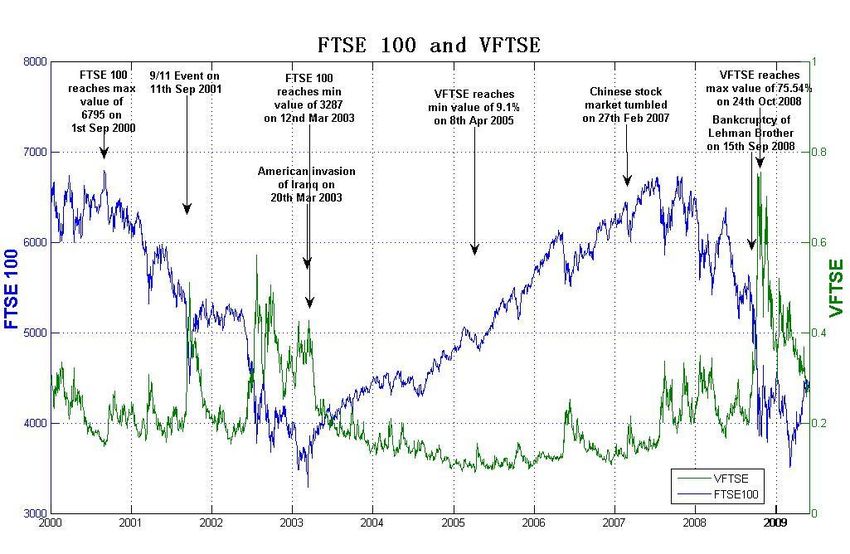
Figure 2 shows the annualised ex post 30 day realised volatility of the FTSE-100 returns
and Euronext VFTSE. These two time series have similar patterns. In most periods,
especially during a boom, the value of realised volatility is lower than the VFTSE.
However, exceptionally, there are also some periods where realised volatility can be
higher than the VFTSE, for example, during the financial crisis at the end of 2008. The25
sample statistics for RV and VFTSE are given in Table 2 along side those for the
constructed IVs.
Figure 2: The realised volatility of FTSE-100 Returns and VFTSE
5.2 Construction of Implied Volatilities of FTSE 100
5.2.1 Carr-Wu IV Method
Following Section 3, we construct the CW- IV for the FTSE-100. We filter the option
data using the CBOE VIX method. Table 1 gives the average number of different daily
strikes with FTSE 100 call and put options for the nearest (1st) and the second nearest
(2nd) maturities. Table A.1 in the Appendix reports the average annual call (Panel A) and
put (Panel B) option prices and number of observations (in brackets) for six different
categories of moneyness ( ) and the two maturities. On average, the nearest maturity
(1st) option prices are lower than the second nearest maturity (2nd) option prices for
almost all moneyness categories for both calls and puts. For the CW-IV, we use all
these option prices to get the Black implied volatilities, and interpolate and extrapolate to26
get finely spaced implied volatility grids as explained in equations (4-6). We then
proceed to construct the CW-IV for the FTSE 100 using equation (8).
Table 1: Yearly Average number of daily strikes
Period Average Number of
Daily Strikes
1st 2nd
Maturity Maturity
2000 92 91
2001 85 81
2002 77 75
2003 60 58
2004 50 50
2005 52 53
2006 55 54
2007 63 58
2008 63 52
2009 a 51 44
[a] The option data for 2009 only includes five months ( 2 January 2009 - 1 June 2009).
5.2.2 Implied Volatilities with GEV and BS (1973)
Following Section 4, for every trading day, the GEV implied parameters are
derived from option prices using equation (20) and constructed to get the annualised
30-day GEV implied volatility with equation (22). In the latter, the constant 30-day
horizon GEV-IV is scaled by using the implied term structure parameter backed out in
(20) from options with all maturities and strike prices available in the market, where their
trading volumes are not zero. This is different from the VFTSE and the implied
volatility model of Carr-Wu derived in section 3, which are calculated using at most only
two options maturities that span the 30 day horizon. For the comparison, we also
construct the standard IVs for the Black and Scholes (1973) model.
5.2.3 Statistical Analysis and Comparison
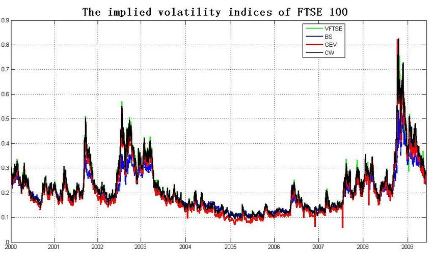
Figure 3 plots the time series of implied volatility indices for the FTSE 100 with the four
different methods (VFTSE, Carr-Wu, GEV, and BS). These four indices show very27
similar patterns with the most obvious visual detail being that the GEV-IV takes on the
smallest values during normal market conditons and the biggest ones during turbulent
conditions. From mid-2003 to mid-2007, the four volatility indices give corresponding
low values, which are mostly below 20%. At the end of 2008, the GEV-IV and CW-IV
peak at around 80% which is similar to the realized volatility in Figure 2. In contrast,
VFTSE peaks at 75% and the BS-IV is the least volatile and peaks at 53%.
Table 2: Summary Statistics of Implied and Realised Volatilities for FTSE 100
Implied Volatility Realised
Volatility
VFTSE BS-IV GEV-IV CW-IV RV
Min 0.0910 0.0954 0.0566 0.0926 0.0512
Max 0.7554 0.5346 0.8229 0.8256 0.7973
Mean 0.2185 0.1982 0.2021 0.2178 0.1831
Std. Dev. 0.1021 0.0717 0.1016 0.1041 0.1155
Skewness 1.5379 1.1900 1.5888 1.6238 2.0594
Kurtosis 6.0321 4.6537 6.4667 6.3989 8.8822
ADF Test # -3.7326 -3.0520 -3.8456 -3.7852 -2.2470
# Augmented Dickey Fuller Test with critical value of -1.942 at 5% significance level (no
constant and time trend)
Table 2 gives the sample statistics of the four implied volatility indices (VFTSE,
Carr-Wu, GEV, and BS) and of the realised volatility of the FTSE-100 The mean of the
VFTSE is 0.2185, while that of the realised volatility is 0.1831. All the other
constructed IV estimates share this property of having a mean greater than the mean of
realised volatility. This is consistent with the findings (see, Anderson and Bondarenko,
2007, and Carr and Wu, 2009) on the negative volatility risk premum which is defined as
the difference between the volatility derived under the P- measure and the volatility
derived under the risk neutral Q-measure. The maximum values for the CW-IV and
GEV-IV are greater than that for the RV while that for the VFTSE it is less at 0.755 and
BS-IV peaks at only 0.53. Their minimum values are all less than 10% , with that for
the GEV-IV at 5.6% being the closest to the minimum of the RV at 5.12%. BS-IV is
much less volatile than the other three volatility indices, and its skewness and kurtosis are
also the smallest of all other IV measures. This fully reflects the assumption of28
log-normality of the model. The RV has kurtosis of 8.82 which is not matched by the
kurtois of any of the IVs. GEV-IV is the closest at 6.46 while the VFTSE has a
relatively low kurtosis of 6.03.
The augmented Dickey-Fuller (ADF) tests (without constant and time trend) in Table 2
show that the four volatility measures and RV all reject the null hypothesis of unit root at
a 5% significance level. This implies that all of these volatility series are stationary.
Also, we apply the Jarque-Bera test (not reported). All five volatility indices reject this
at 5% significance level, indicating none of them is normally distributed. Siriopoulos
and Fassas (2008) also applied the above statistical tests for the VFTSE levels, its
changes and its log changes from February 2000 to May 2008, with similar results.21
Figure 3: The volatility indices of FTSE 100 with the four IV methods:VFTSE,
Carr-Wu IV, GEV-IV, and BS-IV (Jan 2000- June 2009)
The following Figures 5 and 6, respectively, for the implied volatility term structure
21
We also do these tests for the changes and the log changes of the volatility series and find similar results.29 parameter for the GEV-IV model and the time varying implied tail shape parameter, , highlight how GEV-IV produces the smallest values of all the four IVs during normal market conditions while it spikes up rapidly as conditions become turbulent. Using formula (22) for the 30 day horizon GEV-IV and as discussed in Section 4.1 relating to equations (17 and (18), in Figure 5 we see that the registers sudden plunges below 0.5 marking points of abrupt jumps in volatility in September 2001, June 2002, June 2006 and October 2008. The latter gives the lowest point for the implied volatility scale parameter at 0.223 and this coincides with the highest value attained by the GEV-IV. This indicates that the square root of time scaling rule which is true for Gaussian models and one that is used in almost all IV constructions, by permitting linear interpolations of implied variance obtained from option prices of the nearest and second nearest maturity contracts, has substantive implications that warrant closer scrutiny. Figure 5 Option Implied Term Structure Parameter,b, for Scaling GEV-IV Time To Maturity (Jan 2000- June 2009) The implied tail shape parameter, for the GEV-IV model plotted in Figure 6 shows
30

that the maximum value is given by 0 <      < 0.12. This indicates that the      ≈ 0.1
region, large but finite varaince, skewness and kurtosis exists for the GEV RND based
returns through out the sample period. Further,          are by and large a rare events,
with normal conditions with -0.3 <      < 0 being more the norm.      Figure 6 shows that
          during the June/July 2004 correction of the FTSE-100 and then in mid 2005.
From January 2007 to after the Lehman debacle in September 2008,              , showing
market expectations of great turbulence and also large price falls.    During the 2007
period,            in March and June.    In the period after October 2008,     < 0 and with
a very large negative   = - 0.4 occuring in December 2008, marks market expectations of
large upswings in the FTSE-100 in early 2009.     Note, large non-zero values for        result
in increased GEV-IV as skewness and kurtosis also grow.

Figure 6 Option Implied Tail Shape Parameter in GEV-RND Model (Jan 2000-
June 2009)

5.3 Forecasting Realised Volatility with Implied Volatility Indices in FTSE 100
Market
31
The implied volatility is the expectation of future realised market volatility under the risk
neutral measure and hence we have the following relationship (see, Carr and Lee,
2007, Bollerslev, Tauchen, and Zhou, 2008):
(25)
We expect that the implied volatility contains information on ex post realised volatility
defined in (24). In order to verify this, typically linear regressions are run with implied
volatilities as the dependent varable and realised volatility as the independent variable.
We will do this for both the whole sample period and sub-periods.
5.4.1 Estimation for the Whole Sample Period
Univariate Regression
We first run two variants of ordinary least square (OLS) regressions for realised volatility
with the four different IV indices we constructed as respective dependent variables and
also the lagged RV. The first set of regressions are in levels and the second set is in
logarithms of the variables:
(26)
and
(27)
where is the realised volatility at month . stands for the four
volatility indices and lagged realised volatility , respectively.
Christensen and Prabhala (1998) show that overlapping data would exhibit a large
amount of autocorrelation and result in estimation problems and incorrect results.
Therefore, we use non-overlapping RV and IV which are selected from the data once
every month. We choose the last trading day of every month as the observation day.
The implied volatilities (realised volatility) on that day represents the risk neutral
expected volatilities (realised volatility) for the next month. We also use 1 monthYou can also read