Frequency biases in predictions of aviation icing occurrence: What can we learn from climatologies?
←
→
Page content transcription
If your browser does not render page correctly, please read the page content below
Frequency biases in predictions
of aviation icing occurrence:
What can we learn from
climatologies?

Forecasting Research
Technical Report No: 588

22 January 2014
Cyril J. Morcrette (Met Office),
Ben C. Bernstein (Leading Edge Atmospherics, Longmont, Colorado, USA)
and Helen Wells (Met Office)

                                       -1–
       © Crown copyright 2014
Frequency biases in predictions of                              aviation        icing
occurrence:
What can we learn from climatologies?
Cyril J. Morcrette {Met Office, Exeter, UK}

Ben C. Bernstein {Leading Edge Atmospherics, Longmont, Colorado, USA} and

Helen Wells {Met Office, Exeter, UK}

Correspondence to:
Dr Cyril J. Morcrette, Met Office, FitzRoy Road, Exeter, EX1 3PB,
United Kingdom. E-mail: cyril.morcrette@metoffice.gov.uk

Abstract

The prediction of locations where aircraft are susceptible to the accumulation of ice
due to the presence of supercooled liquid water is an important part of the hazard
forecasts provided to aviators. We describe a method for quantitatively assessing the
performance of different icing algorithms by using of model-derived climatologies and
comparing them to climatologies derived from observations. This method helps
identify frequency biases in potential new icing algorithms and helps in their
subsequent development prior to testing in an NWP setting. Our icing-climatology
evaluation method is illustrated by comparing the frequency-of-occurrence biases of
a new icing algorithm to those of the index used operationally. Using the notion that
the actual liquid water content (LWC) encountered by aircraft can be described using
an probability density function describing the fluctuations of the LWC about the
model-predicted grid-box-mean value our new index quantifies the likelihood of
encountering local supercooled liquid water contents above any threshold. Our
evaluation using climatologies then shows that the new index can be tuned to give
unbiased predictions of icing occurrence from a climatological point-of-view. The new
index is shown to capture the variations in icing frequency as a function of month,
height and geographical location as well as the control icing index. However, the new
index has the advantage that its formulation allows for the development of bespoke
icing indices that decouple icing severity and risk. Additionally, the new index can be
interpreted as a probability, allowing it to be incorporated into an ensemble-based
probabilistic forecast.

                                         -2–
© Crown copyright 2014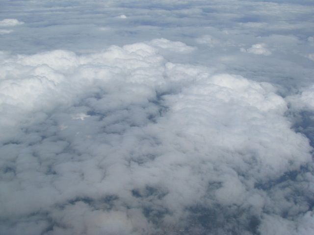
1 Introduction

In the Earth’s atmosphere, water does not necessarily freeze as soon as it is cooled
below 0°C. In the absence of abundant, active ice nuclei, water can exist as a
“supercooled liquid” down to temperatures of around −40°C before homogeneous
nucleation, and freezing, occurs (e.g. Rogers and Yau, 1989). In natural clouds
however, supercooled water is most commonly found at temperatures close to 0°C
and less frequently as temperatures decrease. Using data from a lidar onboard the
space shuttle, Hogan et al. (2004) estimated that, in the latitude range ±60°, there
was liquid water present in around 20% of the clouds whose temperature was
between −10°C and −15°C and that this proportion dropped to essentially zero for
clouds with temperatures colder than −35°C.

When water is in a supercooled liquid state, the introduction of ice nuclei may lead to
the rapid freezing of the liquid onto the nuclei and then onto the newly formed ice
mass. Airplanes, helicopters and other objects such as power lines, antennae and
wind turbines can also act as the surface onto which supercooled liquid water
freezes. The build-up of ice on an aircraft’s structure is known as “aircraft icing” or
simply “icing”. The accumulation of ice on an aircraft’s wings, propellers, fuselage or
external flight instruments can have a negative impact on its manoeuvrability and
performance with potentially catastrophic consequences (e.g. Politovich, 2003; Cole
and Sand, 1991; Lankford, 2001).

Since aircraft icing is due to the presence of supercooled liquid water in the
atmosphere, then meteorologically, the problem becomes one of predicting the
existence of clouds in the right temperature range, then differentiating between those
clouds that are likely to be dominated by supercooled liquid, rather than ice.
Automated icing forecasts are typically produced taking temperature and humidity
information from a numerical weather prediction (NWP) model. As a result the quality
of the icing forecast is very dependent on the realism of the temperature and
humidity which the model predicts will prevail at a particular time and place
(Thompson et al., 1997).

Bernstein et al. (2005) reviewed different icing diagnosis and forecasting techniques.
Some methods, based purely on NWP model temperature and humidity, without
including information about the cloud cover and liquid water content, tended to
overpredict the occurrence of icing and would sometimes predict icing in regions
which were actually cloud-free. To mitigate this issue, Tafferner et al. (2003), Le Bot
(2004) and Bernstein et al. (2005) developed icing indices that combined
temperature and humidity information from short-lead-time NWP forecasts with cloud
observations from satellite and reflectivity information from ground-based radar.
These algorithms all employed a scenario-based approach, while Bernstein et al.
(2005) also used fuzzy logic membership functions to capture some of the inherent
uncertainty and variability in both icing probability and severity. McDonough et al.
(2004) and Wolff et al. (2009) extended this approach to develop forecasts of icing
out to 18 hours.

It is common to evaluate icing forecasts using aircraft observations of icing, such as
pilot reports (PIREPS), since these are a strong, fairly direct indication of the
phenomenon being forecast (Brown et al., 1997). There are issues with using
PIREPS however. Firstly, PIREPS of icing conditions exhibit spatial and temporal
patterns that are artifacts of air-traffic density and the daily and weekly pattern in the
number of flights that occur (Schultz and Politovich, 1992). Secondly, PIREPS of “no
icing” are under-represented because pilots are more likely to report the presence of

                                          -3–
© Crown copyright 2014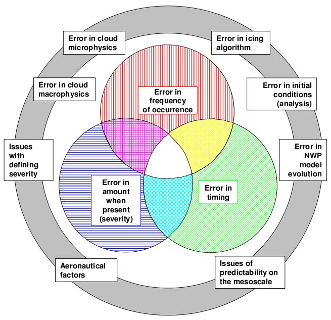
icing rather than its absence. Although it is possible to infer the absence of icing
conditions from some of the other information contained in the PIREPS, any
statistical evaluation of icing algorithms must be done with careful consideration of
these sampling biases (Brown et al., 1997). Finally, PIREPS do not provide an easy
means of assessing the severity of an icing forecast. This is because the PIREPS of
icing severity are subjective in nature and represent a combination of the
meteorological environment, the aircraft type, the ice protection system, how it is
applied, flight history and pilot perception (Sand and Biter, 1997).

Morcrette et al. (2012) discussed the evaluation of cloud cover forecasts and the
different types of cloud forecast errors. Their conclusions can also be applied to the
evaluation of icing forecasts and so Fig. 1 shows a Venn diagram illustrating the
different ways in which an icing forecast can be in error. When assessing the
statistical performance of an icing forecast over a long period, the forecast can be
incorrect due to an error in: i) frequency of occurrence (FOO) of icing conditions, ii)
amount when present (AWP, i.e. the severity of icing when icing is predicted) and iii)
timing. As an example of the different aspects of the icing forecast error, an icing
forecast could over-predict the FOO of generic icing conditions, but under-predict the
AWP, or severity, leading to the FOO of severe icing conditions actually appearing to
be quite accurate. Averaged over a long period, an icing index could also correctly
predict the FOO and the severity in a mean sense, but get the timing wrong, for
example, by consistently predicting icing too early or late in the day.

When assessing the skill of a large number of icing predictions statistically all three
error components will be present (as illustrated by the white region in the centre of
the Venn diagram). In order to improve the performance of an icing prediction
system, one needs to think about the sources of the errors. Inaccuracies in icing
predictions can be due to a variety of causes, as shown around the perimeter of Fig.
1. An icing prediction can turn out to be wrong because of errors in the model’s
microphysics, the model’s grid-resolved condensate amount and fractional cloud
cover or the icing algorithm. It can also be wrong due to errors in the large-scale
thermodynamic state, either because of errors in the model evolution or due to the
analysis used to initialise the forecast. The severity of an icing risk can also appear
wrong due to issues to do with defining severity and the degree to which icing
severity is influenced by aeronautical as well as meteorological factors.

One reason for measuring the skill of any forecast is to compare the relative
performance of two systems. This helps when developing new forecasting methods
as it enables a comparison with the current operational system. Quantitative
measures of relative performance can also be used when deciding to replace an
operational product with a newly-developed one.

This paper argues that it is important to know which aspects of the icing forecast
error a particular evaluation method is sensitive to. Additionally, one should aim to
have an icing-forecast evaluation method that measures these different aspects of
the icing forecast errors. This is because certain measures of skill are very sensitive
to one aspect of the error. If one only considers a single skill metric, one can get a
misleading picture of the relative performance of two forecasting systems. If one
makes improvements to the aircraft icing algorithm, in order to tackle one aspect of
the forecast error but only assesses it using a metric that is very sensitive to another
aspect of the error, which has not changed, then one can be misled as to whether the
changes made to the algorithm have actually improved anything. Icing forecasts can
be evaluated using the Equitable Threat Score (ETS or Gilbert Skill Score, Gilbert
(1884)) which quantify the skill with which observed events were forecast. However
this skill score is very sensitive to timing errors and the double penalty effect. This is

                                          -4–
© Crown copyright 2014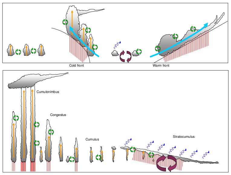
aside from the fact that the Equitable Threat Score turns out not to be equitable
(Hogan et al., 2010).

Since icing indices tend to be so dependent on the model’s prediction of temperature
and humidity (Thompson et al., 1997) then if there is a timing error in the model’s
large-scale flow, for example due to problems with the model’s initial conditions, or
due to the incorrect evolution of the atmosphere caused by problems with the
model’s physical parametrization schemes, then that error will still be present no
matter how the icing forecast algorithm is re-formulated. As a result comparing the
relative performance of two icing algorithms by using the ETS will not be particularly
informative.

So out of the three aspects of the icing forecast error: timing, severity and frequency
of occurrence, it seems that evaluating the frequency of occurrence may be the most
helpful from the point of view of developing and testing potential new aircraft icing
indices.

Bernstein et al. (2007) and Bernstein and Le Bot (2009) describe climatologies of
icing conditions inferred from several years’ worth of surface weather reports, balloon
soundings and model re-analyses. These icing climatologies estimate the frequency
of occurrence of icing conditions geographically and as a function of height and
month of the year for 15 sites around the world (Fig. 2). The patterns found in these
studies compared favourably with large independent datasets of observed icing from
PIREPs over the U.S. and surface observations from mountain sites in Europe.

The Met Office has a seamless forecasting system (Brown et al., 2012), which
means that there is a general circulation model (GCM) configuration which can be
used for operational global NWP and that the same model and choice of
parametrization schemes can be used to perform global climate simulations. This
configuration is known as Global Atmosphere 3.0 (GA3.0, Walters et al., 2011). In
this study, a multi-year simulation of the present-day climate will be used as input to
a variety of icing algorithms. This will enable us to determine the frequency of icing
conditions at the 15 locations documented in the climatologies as predicted by each
algorithm. The various icing algorithms will then be assessed in terms of their ability
to reproduce the site-to-site, monthly and altitude variations of the inferred icing
climatologies derived from indirect observations. The various icing algorithms will be
assessed specifically in terms of the error in their frequency of occurrence (see Fig.
1). That is to say, the icing algorithms will be evaluated in terms of their ability to
predict the frequency of occurrence of the inferred icing climatologies derived from
indirect observations, including their ability to reproduce the site-to-site, monthly and
altitude variations. Although we do not suggest that a new icing algorithm can be
verified solely by using a climatology, we believe that the evaluation of the model-
predicted icing climatology is an important step in assessing the performance of any
new icing algorithms.

One of the important features of GA3.0 compared to the previous global operational
NWP model configuration is the inclusion of the prognostic cloud, prognostic
condensate, cloud scheme (PC2, Wilson et al., 2008a). This scheme has been
shown to lead to an improved representation of cloud in both the climate (Wilson et
al., 2008b) and weather forecasting context (Morcrette et al., 2012). The PC2 cloud
scheme has 5 prognostic variables: liquid and frozen condensate and liquid, frozen
and total cloud fraction. Due to the presence of mixed-phase regions, the total cloud
fraction is not necessarily equal to the sum of the liquid and frozen cloud fractions.

                                          -5–
© Crown copyright 2014
The PC2 scheme calculates sources and sinks for each of these prognostics
variables and advects the updated cloud variables using the model winds. Each of
the following physical processes can modify the cloud fields: short-wave radiation,
long-wave radiation, boundary-layer mixing, precipitation formation (microphysics),
sub-grid-scale convective motions, sub-grid-scale mixing (erosion) and grid-resolved
ascent and adiabatic cooling (Wilson et al., 2008a). The microphysics scheme in the
MetUM (Wilson and Ballard, 1999; Walters et al., 2011) considers a number of
physical processes including homogeneous and heterogeneous freezing,
depositional growth, fall, melting and sublimation of ice. It also includes
autoconversion and accretion of liquid water to rain and riming of liquid, capture of
raindrops by ice and evaporation of rain.
Following Morcrette and Petch (2010), Fig. 3 uses annual-mean global cloud-scheme
process rates to show the relative contribution of each parametrized physical process
to the sources (Fig. 3a) and sinks (Fig. 3b) of liquid water content and to the sources
(Fig. 3c) and sinks (Fig. 3d) of liquid cloud fraction. The PC2 cloud scheme
represents the impact of all these physical processes that can create and remove
cloud and is designed to represent all cloud types: from large-scale cloudiness
associated with synoptic-scale ascent, to the partial cloudiness, and relatively high in-
cloud water contents, associated with convective regimes. Using data from the
quantitative studies of Morcrette and Petch (2010) and Morcrette (2012b), Fig. 4
provides a schematic of the dominant cloud source and sink terms that are acting in
different cloud regimes. In the mid-latitudes, the convection scheme is a source of
cloud in the cold sector of extra-tropical cyclones and along the cold front. Large-
scale ascent is also important along both the cold and warm fronts. Boundary-layer
mixing is an important cloud-formation process in the warm sector. The formation of
precipitation within the cloud, and the cloud erosion associated with the mixing of
clear and cloudy air at cloud edges, are the main sink terms for liquid cloud. When
considering a cross-section from sub-tropical stratocumulus to tropical deep
convection one finds that the stratocumulus cloud decks are replenished by long-
wave cooling from cloud top and boundary-layer mixing. These source processes are
offset by cloud erosion and the microphysical transfer of cloud water to precipitation
which then falls out of the cloud. As the boundary-layer and long-wave cooling
sources diminish, the cloud regime often transitions to broken shallow convective
clouds where the convection scheme becomes a key source term. In the tropics, the
dominant cloud creation process is convection, which is balanced by sinks from
microphysics and cloud erosion.
As one of only two World Area Forecasting Centres (WAFC), the Met Office (referred
to as WAFC-London) provides forecasts of the risk of en-route icing conditions for
use by aviation. The use of the new PC2 cloud scheme in the operational global
forecast model is the perfect opportunity to revisit the icing algorithm currently being
used and to ask whether a better forecast algorithm could be developed that makes
use of the improved temperature, cloud and humidity fields produced by the new
model configuration and which could be incorporated into an ensemble-based
probabilistic forecasting system. The first step in our icing index development
strategy is to consider how a new icing index might be evaluated. This paper
describes a method for evaluating the frequency of occurrence characteristics of
proposed new icing indices. This is demonstrated by developing and testing a series
of hypothetical new icing indices and showing that, from a statistical point of view,
some of them can perform as well as the current operational (control) algorithm.
The current WAFC-London icing algorithm is reviewed in Section 2 before describing
a series of potential new indices of increasing complexity. In section 3 we present a
method for the statistical evaluation of proposed icing indices from a climatological
-6–
© Crown copyright 2014point-of-view and illustrate its use by showing that one of these new indices, which
has a much better scientific basis, can perform as well as the current index, when
assessed against the climatologies. Section 4 provides a discussion. A summary and
conclusions are given in Section 5.
2 Description of icing indices (II)
2.1 Some existing icing indices
Several icing indices (II) are considered in this paper and are listed in Table 2 in
order of increasing complexity. In each case the algorithm starts by assigning the II a
default value of zero to each location in space and time. Then, using data from an
NWP forecast, the algorithm considers each model grid-box at each output time and
checks whether the temperature is in the range of 0 to −20°C. If it is, the numerical
value of the II is set based on information about the local humidity or cloud. Finally,
the algorithm checks whether the II is above a critical value, iicrit. If it is, then the
algorithm is predicting an icing risk. The critical value can be different for each II,
reflecting the statistical properties of each, which depend on how it is defined.
One method of calculating an II is the “Class I” algorithm described by Schultz and
Politovich (1992). For those points whose temperature is between 0 to -20°C, the
icing index is set equal to the relative humidity (RH). This II based on RH is referred
to as II(RH) in Table 2. The icing index currently used in the Met Office/WAFC-
London products is similar to the “Class I” algorithm of Schultz and Politovich (1992).
For grid-points in the right temperature range, the algorithm checks if the three-
dimensional cloud fraction field is greater than zero. If there is cloud present, the
three-dimensional icing index is set to the RH. This index, based on RH if cloud is
present, will henceforth be referred to as II(RHCldPres).
2.2 Some other icing indices
One feature of II(RH) and II(RHCldPres) is that they are both dimensionless and
typically have a value between 0.0 and around 1.0. In practice however, the lower
limit of II(RHCldPres) is determined by the critical RH required for cloud to form in the
model. This critical RH is usually between 0.8 and 0.95 and is generally specified, or
calculated, as part of the fractional cloud cover parametrization scheme. As a result
of II(RH) and II(RHCldPres) being dimensionless and typically having values
between 0.0 and 1.0 they have sometimes been interpreted as a probability.
However, this is not how these indices should be used. This is because there is no
reason why the grid-box-mean RH should directly quantify the chance of
encountering icing conditions within a grid-box. Additionally, although large
supersaturation with respect to liquid is rare in the atmosphere, RH values greater
than 1.0 do have a physical meaning. An II based on RH could in principle report
values greater than 1.0, but these would make no sense if the II is interpreted as a
probability. In practice, the II(RHCldPres) is capped at 1.0, within the icing algorithm
code, prior to being disseminated to WAFC-London for use in producing the icing
forecast.
General circulation models used for global NWP make use of cloud parametrization
schemes to determine the fraction of the model grid-box which is covered by cloud
based on information about the local thermodynamic state (e.g. Smith, 1990) and,
increasingly, using information about the other physical processes occurring at the
same location (e.g. Tiedtke, 1993; Tompkins, 2002; Wilson et al., 2008a; Watanabe
et al., 2009).
-7–
© Crown copyright 2014In the next sub-section, a proposed new icing index is described. This will make use
of information about both the grid-box fractional cloud cover and the grid-box-mean
liquid water content. However, before describing the relatively complex index which
uses both of these inputs, it seems sensible to check whether the same inputs could
be used directly to develop a simpler icing index.
The model grid-box’s cloud fraction (CF), that is the fraction of the grid-box which is
covered by cloud, is an intuitive choice as an input for a potential new II. This will be
referred to as II(CF) and we note that in this case the algorithm is using the generic
cloud fraction, which means it is not distinguishing between condensed water in the
liquid or ice phase. In the MetUM, the liquid cloud fraction (LCF) is available as a
separate variable. This allows us to consider a slightly different index, II(LCF), which
is based on the fraction of the grid-box containing condensate in the liquid phase.
One feature of the PC2 cloud scheme is the relative independence with which the
LCF and liquid water content (LWC) can vary. Although the existence of non-zero
LCF must imply non-zero LWC and vice-versa, the PC2 scheme is able to produce a
wide range of LWC for a given LCF (Wilson et al., 2008b). As a result, it is
reasonable to consider whether using grid-box-mean LWC as an input would
produce a significantly different new II. This will be called II(LWC), where the LWC is
in gm-3 rather than kg kg-1.
For the purposes of developing icing indices, it is useful to consider the minimum
supercooled LWC, qτ, which poses a risk to aviation. Although this minimum value
will vary depending on the aircraft and also depends on the presence of supercooled
large drops, which are not considered here, a value of qτ = 0.1gm-3 seems a sensible
threshold and is consistent with the values reported by Politovich (2003) and with
those used in the wind-tunnel studies of Ide (1999).
To aid comparison with the other II, II(LWC) is normalised by dividing by 2qτ. This
means that II(LWC) will be dimensionless and will have a value of 0.5 if the grid-box-
mean LWC, qcl, is equal to the threshold LWC, qτ.
The grid-box-mean LWC, qcl, is the value of LWC that one would obtain if the
condensed water was distributed evenly across the grid-box. As we have seen
however, the model also predicts the LCF, Cl, so a more sensible variable for use in
an icing index is the mean LWC within the clouds, that is the in-cloud LWC (icLWC),
which is defined as qcl/Cl. This index, which is also normalised by dividing by 2qτ, will
be called II(icLWC).
Even within the cloudy portion of a grid-box however, there is considerable variability
in the amount of condensate. The importance of this variability on the clouds’
radiative impact (Cahalan et al., 1994) has led to the development of radiation
schemes, such as the Monte Carlo Independent Column Approximation (McICA),
which sample this variability (Pincus et al., 2003). From the point of view of
forecasting icing conditions, the variability in sub-grid-scale supercooled LWC is likely
to be very important. Indeed, just because the mean in-cloud LWC is below a given
threshold does not mean that the threshold is not exceeded anywhere within the grid-
box.
By assuming that the sub-grid cloud variability can be described by an analytic
function, Räisänen et al. (2004) generated a sample of sub-grid-scale cloudy
conditions, consistent with the grid-box-mean cloud cover, condensate amount and
some information about the standard deviation of the condensate. These were then
used when performing radiation calculations.
-8–
© Crown copyright 2014In the next sub-section, we use similar ideas about the sub-grid-scale variability in
LWC to develop a new icing index that quantifies the probability of encountering
supercooled LWC above a certain threshold somewhere within the model grid-box.
2.3 A proposed new icing index
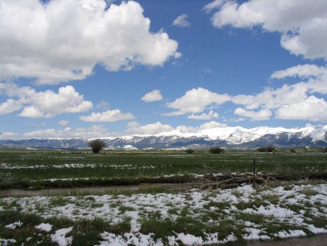
Figure 5 shows some photographs of clouds containing supercooled liquid water. In
an NWP model, these cloud fields could typically be represented by only a single
grid-box in the horizontal. This grid-box would have a single value of fractional cloud
cover, Cl, and a single grid-box mean liquid water content, qcl. There is variability in
the real cloud field however and some parts of the clouds may have a high enough
liquid water content that they pose a risk to aviation while some parts will have much
lower liquid water content. Some portion of the grid-box may be altogether cloud-free.
To demonstrate the use of climatologies in evaluating potential new icing indices, we
have developed a new icing index which aims to estimate the fraction of the model
grid-box that contains local liquid water content, qcl, above a certain threshold, qτ.
Following Räisänen et al. (2004), we assume that within the cloudy part of the grid-
box, the variability in the local water content, qcl, can be described by an analytical
probability density function (PDF), which we will call P(qcl). The mean value of this
PDF is set to the mean in-cloud LWC, calculated by dividing the grid-box mean LWC,
qcl, by the liquid cloud fraction, Cl. Later, it will also be necessary to specify the
fractional standard deviation of the sub-grid variability. This PDF is then integrated
between the limits of the threshold LWC, qτ, and infinity, using some analytical
solutions. This integral will give, F, the fraction of the cloudy region with LWC above
the threshold. The fraction of the sky with LWC above the threshold, or the chance
(χ) of encountering local LWC above the threshold, is then found by multiplying this
integral, F , by the grid-box-mean liquid cloud fraction, Cl:
∞
χ (qτ ) = F (qτ )Cl = Cl ∫ P(qcl )dqcl
qτ
Equation 1
The concept behind the χ icing index is illustrated in Fig. 6 using a gamma PDF, a
mean in-cloud water content of qcl/Cl = 5.0 × 10⁻⁵ kg kg-1 and a fractional standard
deviation, fc = 0.75. The threshold LWC is 1.0 × 10⁻⁴ kg kg-1 and the portion of the
PDF where the local LWC is greater than the threshold, around 10% in this case, is
shaded in Fig. 6a. It is worth noting that although the mean is half the threshold
value, while the mode is smaller still, a part of the cloud is expected to have local
LWC above the threshold value because of the PDF’s long tail. An example of the
variability in local LWC across a model grid-box with a cloud cover of Cl = 0.5 is
shown in Fig. 6b. In this example, there are 200 samples, which are randomly
determined to be cloudy or clear, and if cloudy their LWC is taken from the gamma
PDF. Despite, the cloud only covering 50% of the grid-box and the mean in-cloud
water content being half of the threshold value, around 5% of the grid-box has a local
LWC higher than the threshold. This is a non-negligible amount. It is this aspect of
sub-grid variability in LWC and its link to aircraft icing that we wish to build into our
new algorithm.
The rest of this subsection describes the functional form of the LWC PDF, documents
the parametrization of the standard deviation that will be used in calculating it and
explains the numerical techniques used for integrating Equation 1.
-9–
© Crown copyright 20142.3.1 Justification for using analytical PDF
Ground-based remote-sensing observations of liquid water cloud are used to infer
the sub-grid-scale variability in LWC. The observations were made at the
Atmospheric Radiation Measurement (ARM, Stokes and Schwartz, 1994) or Cloud-
Net (Illingworth et al., 2007) sites at Chilbolton, Darwin, Lindenberg, Murgtal and the
Southern Great Plains (Oklahoma) during the month of April 2007 as described in
(Morcrette et al., 2012). The observed LWC were averaged onto the MetUM grid in
the vertical. The observations were also averaged in time, using the model wind-
speed, for the time it would take a cloud to be advected the length of the grid-box.
This time-averaging creates a horizontal sample comparable to the size of the GCM
grid-boxes used in the simulations described in Section 3.
In order to compare the PDF of LWC from grid-boxes with a large variation in grid-
box mean LWC, the individual LWC observations have been normalised by the
corresponding grid-box mean LWC before calculating the PDF. Figure 7 shows the
observed PDF of LWC within a grid-box, alongside a gamma and log-normal PDF
which have the same mean and standard deviation as the observed PDF. Both
analytical PDFs are a fair representation of the observed distribution, although both
produce a mode smaller than the mean, which is not seen in the observations. The
gamma distribution, however, is better at capturing the probability of the mode.
Using a gamma PDF within an icing algorithm has the advantage that conceptually
the assumptions about sub-grid variability would then be consistent with the cloud-
generator which is used by McICA and which have been included into the MetUM
radiation parametrization scheme (Hill et al., 2011). For completeness, however, we
include the description of the icing index derived using both the gamma and log-
normal PDF assumptions and compare both of them to the observed climatology.
2.3.2 Gamma distribution
The variability in LWC within the cloudy part of the grid-box can be defined by a
gamma distribution given by:
1
P (x ) = x k −1e − x / θ
Γ(k )θ k
Equation 2
where k and θ are the shape and scale parameters respectively. The mean, m, and
variance, v, of the variable x are given by
m = kθ
Equation 3
and
v = kθ 2
Equation 4
which can be re-arranged to give θ and k in terms of m and v:
θ = v/m
Equation 5
and
- 10 –
© Crown copyright 2014k = m /θ
Equation 6
2.3.3 Log-normal distribution
Alternatively, the in-cloud LWC variability can be represented using a log-normal
distribution given by:
(ln( x )− µ )2
1 −
2σ 2
P (x ) = e
x 2πσ 2
Equation 7
where µ and σ are the mean and standard deviation of the logarithm of the variable
x. The mean, m, and variance, v, of the variable x are given by
σ2
µ+
m=e 2
Equation 8
and
( 2
v = eσ − 1 e 2 µ +σ ) 2
Equation 9
which can be re-arranged to give µ and σ in terms of m and v:
1 ⎛ v ⎞
µ = ln(m ) − ln⎜ 2 ln (m )
+ 1⎟
2 ⎝ e ⎠
Equation 10
and
σ = 2 ln(m) − 2µ
Equation 11
2.3.4 Closing the LWC PDF parametrization
Since we are considering the PDF of in-cloud LWC, the mean value of the PDF, m, is
set equal to the mean in-cloud LWC derived from the grid-box mean LWC, qcl, and
grid-box mean liquid cloud fraction, Cl:
q cl
m=
Cl
Equation 12
Now the variance, v, of the PDF, is the square of its standard deviation, s.
Additionally, the fractional standard deviation of the condensate, fc, is defined as the
standard deviation, s, divided by the mean, m, so
2
v = s 2 = (mf c )
Equation 13
In order to complete the parametrization of the sub-grid-scale LWC variability we
need to specify the fractional standard deviation, fc, of the PDF.
Following on from the work of Hill et al. (2012), remote-sensing data collected by
Cloud-Sat, Cloud-Net/ARM and in-situ observations made by atmospheric-research
- 11 –
© Crown copyright 2014aircraft were used by Boutle et al. (2013) to derive a parametrization for the fractional
standard deviation of LWC as a function of grid-box size and cloud cover. This
parametrization takes the form of:
⎧(0.54 − 0.25Cl )φc (x, Cl ) Cl < 1
f c = ⎨
⎩ 0.11φc (x, Cl ) Cl = 1
Equation 14
where
( )
φ (x, Cl ) = (xCl )1/ 3 (0.06 xCl )1.5 + 1
−0.17
Equation 15
and x is the size of the grid-box in kilometres. The variation of fc as a function of
cloud fraction and grid-box size is illustrated in Fig. 8. The Boutle et al. (2013)
parametrization of fc is used here to close the gamma and log-normal PDFs for use in
two new icing algorithms called II(χ-Γ) and II(χ-LN), respectively.
2.3.5 Fraction of cloud with LWC above threshold
Having specified a LWC PDF, P(qcl), the fraction of cloud, F, with a local LWC above
a certain threshold qτ is:
∞
F = ∫ P(q cl )dq cl = 1 − CDF (qτ )
qτ
Equation 16
where CDF is the Cumulative Density Function given by:
qτ
CDF (qτ ) = ∫ P(qcl )dq cl
0
Equation 17
For a gamma distribution, the CDF is given by
1 ⎛ qτ ⎞
CDF (qτ ) = γ ⎜ k , ⎟
Γ(k ) ⎝ θ ⎠
Equation 18
where γ(k, qτ /θ) is calculated from the lower incomplete gamma function, defined as
s −x
∞
xn
γ (s, x ) = x Γ(s )e ∑
n =0 (s + n + 1)
Equation 19
In the icing algorithm, this is calculated by doing the summation up to n = 20. An
example of a gamma distribution and its associated F = 1−CDF is shown in Fig. 9.
Alternatively, if the PDF is defined by using a log-normal distribution then the CDF is
given by:
1 1 ⎛ ln(qτ ) − µ ⎞
CDF = + erf ⎜ ⎟
2 2 ⎜⎝ 2σ 2 ⎟
⎠
Equation 20
where erf is the error function defined as:
- 12 –
© Crown copyright 2014x
2 −t 2
erf (x ) = e dt
π ∫ 0
Equation 21
Using Taylor expansion this can be written as:
erf (x ) =
2 ∞
(− 1)n z 2n+1
π
∑
n =0 n!(2n + 1)
Equation 22
In the icing algorithm this is implemented by expanding up to the 13th order:
2 ⎛ x3 x5 x7 x9 x11 x13 ⎞
erf (x ) = ⎜⎜ x − + − + − + ⎟
π ⎝ 3 10 42 216 1320 9360 ⎟⎠
Equation 23
An example of a log-normal distribution and its associated F = 1−CDF is also shown
in Fig. 9.
The variation in F = 1−CDF as a function of liquid cloud fraction and liquid water
content for a sub-grid variability defined using a gamma and log-normal PDF is
shown in Fig. 10(a and b). In both cases the fractional standard deviation, fc, is
assumed to be 0.75. Multiplying by the liquid cloud fraction gives χ which is shown in
Fig. 10(c and d).
Throughout this paper, χ is calculated using a threshold of qτ = 1.0 × 10⁻⁴ kg kg-1 . If a
different threshold were to be used, we propose that the term χ-LN or χ-Γ should be
followed by the qτ threshold used in calculating it, i.e. χ-Γ(1.0 × 10⁻⁴ ).
3 Calibration of model-derived icing indices using observed climatology
3.1 Method
The icing indices listed in Table 2 and described in Section 2 will be assessed by
comparing their climatologies as a function of location, height and time of the year
against some climatologies inferred from observations. Bernstein et al. (2007) and
Bernstein and Le Bot (2009) produced month-height plots of the frequency of icing
conditions aloft at 15 sites world-wide. The data from these two climatologies are
shown in Fig. 2 while the locations of each of the sites are given in Table 1.
It is worth noting that the vertical axes in Fig. 2 are with respect to sea-level. The
altitude of each site is given in Table 1 and is indicated by the thin black line across
the bottom of each panel. In many cases, the site is near enough to sea-level that the
black line is not discernibly higher than the x-axis. At Guiyang, which is 1074 m
above sea-level, the absence of an icing occurrence below 1 km simply reflects the
altitude of the site. Similarly, Denver, with an altitude of 1655 m, does not have any
icing occurrence below 1 km. The icing that occurs between 1 and 2 km above sea-
level must however all actually be occurring between 1655 and 2000m, that is
between 0 and 345 m above ground level.
For this study, the MetUM has been run as an atmosphere-only climate model,
forced by observed sea-surface temperatures. The simulation starts on 1 Sept 1981
and runs for 20 years and 3 months. The first 3 months are then discarded to allow
for spin-up.
- 13 –
© Crown copyright 2014A detailed description of the package of atmospheric parametrizations used in the
GA3.0 configuration is given by Walters et al. (2011). For our purposes, we note that
the model uses the PC2 cloud scheme (Wilson et al., 2008a,b). The model is run
using the L85 vertical grid, which has 85 vertical levels, 50 of which are below 18km
and the model top is at a height of 85 km. The horizontal resolution is N96, leading to
a regular latitude-longitude grid of 145 × 192 points. For the 15 sites being
considered the mean grid-box dimension is around 138 km.
At each of the 15 sites that appear in the climatologies of Bernstein et al. (2007) and
Bernstein and Le Bot (2009), profiles of temperature, humidity, pressure, density,
liquid cloud fraction, generic cloud fraction and liquid cloud condensate are output
from the model. These are output every 20 minute timestep for the entirety of the 20
year run. The information from all of these thermodynamic profiles is then used to
calculate what each of the 8 icing indices in Table 2 would predict at that place, time
and height.
Then for each site, we go through the 20 years and check whether the icing index is
above a certain threshold. If it is, the icing index is assumed to have “predicted icing
conditions”. We then calculate the frequency of predicted icing conditions for each
height and month, by looking at the entire 20-year period. This analysis considers 11
thresholds in turn: 0.01, 0.02, 0.05, 0.10, 0.20, 0.40, 0.60, 0.80, 0.90, 0.95, 0.98 and
the procedure is repeated for each of the 8 icing indices.
3.2 Results
Figure 11 shows profiles of frequency of icing conditions for each of the icing indices
and each of the thresholds. The profile of observed frequency of icing conditions,
averaged over all the sites and months is shown for comparison. The first thing to
note is that although all the icing indices produce values between 0 and 1, the
distribution of values produced by each index is very different. As a result, the value
of the icing index above which the index should be interpreted as having predicted
icing conditions will be different for each index. Consequently, if one replaces one
index by another within an operational system, the threshold value will also need to
be changed.
As an example the current icing index, II(RHCldPres), reproduces the observed
profile of icing conditions the best when using a critical value of around 0.95
(magenta) and over-predicts the occurrence of icing when using a threshold below
that (Fig. 11b). The index based on generic cloud fraction, II(CF), matches the
observed climatological frequency of icing occurrence quite well when using a
threshold of 0.6 (blue, Fig. 11c) however this leads to an overprediction at heights
below 2 km. II(LCF) and II(LWC) both match the observed profile above 3 km quite
well when using a critical value of around 0.1 (green) although they then overpredict
icing occurrence below that height (Fig. 11d and e). The two version sof the χ index
give very similar results, as is to be expected since the only difference between them
is whether the sub-grid-cloud variability is represented using a log-normal or gamma
PDF.
The two icing indices based on χ also both capture the shape of the icing frequency
profile above 3 km when using a critical value of 0.02 (orange), however they also
both over-predict the frequency of icing conditions below 3 km. This over-prediction
in the frequency of occurrence of icing conditions at lower levels is consistent with
the over-prediction of the frequency of occurrence of low and mid-level liquid cloud
identified by Morcrette et al. (2012) when comparing predictions of cloud cover using
- 14 –
© Crown copyright 2014GA3.0 to observations from ARM and Cloud-Net sites. Consequently, the over-
prediction of icing conditions exhibited by the χ indices is not thought to be a
deficiency of the χ algorithm, but rather, it is related to a cloud bias seen in the host
model. Future developments of the GA configuration, such as changing the
formulation of liquid cloud erosion (Morcrette, 2012a), may improve this bias.
We now investigate the ability of each of the icing indices to reproduce the observed
climatologies in terms of the variation in frequency of occurrence of icing as a
function of location, height and month. For each icing index, we consider the time-
height climatologies shown in Fig. 2, and calculate the bias and root-mean-squared
error (RMSE) between the frequency of occurrence predicted by each index and the
frequency of occurrence inferred from the observations. This comparison is done
using icing index thresholds ranging from 0.01 to 0.99 in steps of 0.01 and is
repeated for each of the icing indices (Fig. 12).
The control icing index II(RHCldPres) has zero bias when using an iicrit value of
around 0.96. II(CF) has zero bias when using a critical value of around 0.62, while
values of 0.10, 0.12 and 0.80 lead to unbiased frequency of occurrence using
II(LCF), II(LWC) and II(icLWC), respectively. The χ-LN and χ-Γ indices have no bias
when using iicrit values of around 0.06. The ability of the icing algorithms to reproduce
the observed climatology can also be quantified by looking at the RMSE in the
frequency of occurrence, hence quantifying the ability of the indices to predict the
correct variation of icing frequency with height and month of the year. All the indices
tend to have lower RMSE as their biases are reduced, however the critical value
which leads to the lowest bias does not lead to the lowest RMSE and vice versa (Fig.
12). Interestingly, the magnitude of the smallest RMSE that can be achieved by each
index is very similar. Additionally, the RMSE associated with an unbiased χ
prediction is comparable to the RMSE associated with an unbiased prediction using
the control algorithm, II(RHCldPres). So by using an appropriate value of iicrit , the χ
indices can perform as well as the operational control index from the point of view of
long-term statistics.
For each icing index, we can then find the iicrit values which lead to unbiased
prediction of icing frequency when compared to climatology when assessed over all
the sites, months and heights. Figure 13 shows the time-height plots of icing
frequency predicted by the control icing index, II(RHCldPres), when using an iicrit of
0.96 to determine that icing conditions are likely. Figure 14 shows the time-height
plots using the new χ-Γ algorithm and an iicrit of 0.06. The climatology produced using
the II(χ-LN) algorithm, and a critical value of 0.06, is very similar to the one produced
using II(χ-Γ) using the same critical value (not shown). The fact that the overall
frequency of occurrence for both model-derived climatologies is comparable to the
observed climatology simply reflects the fact that, in this analysis, the model-derived
indices have been calibrated against the observational data. However, this is the first
time that a potential icing algorithm for use in NWP has been calibrated in this way
and it may prove to be a useful part of the icing index development process.
Visual comparison of the model-predicted icing climatologies (Figs. 13 and 14) with
the observed climatology (Fig. 2) shows that the two icing index climatologies
computed from climate model output are capable of reproducing the broad features
of the variability of icing frequency as a function of height, month and geographical
location.
As before, we note that the vertical axes in Figs. 13 and 14 are with respect to sea-
level. The height of the model orography at the locations used in the climatology
does not necessarily match the height of the true orography. This is due to the desire
- 15 –
© Crown copyright 2014to avoid orographic forcing near the grid-scale, which can compromise the stability of
the numerical model. As a result, the orography is smoothed, however this is not a
trivial exercise as one wishes to maintain the height of important mountain ridges,
while preventing sea points from being raised above sea-level (e.g. Rutt et al., 2006).
The height of the model orography at the model grid-point nearest to each of the
sites is indicated by the thin black line across the bottom of each panel in Figs. 13
and 14. In most cases, the model orography and true orography are within 200 m of
each other. One notable exception is Denver. Since it is only 25 km east of the edge
of the Rocky Mountains the nearest grid point has a height of 2446 m, nearly 800 m
higher than the true orography. As a result, the lowest altitude above sea-level the
140 km grid-length model can predict the occurrence of icing at Denver is 2446 m.
This explains the absence of predicted icing between 1 and 2 km in Figs. 13e and
14e.
4 Discussion
Closer comparison between Figs. 2, 13 and 14 reveals a number of interesting
results. The II(RHCldPres) algorithm fails to predict any icing occurrence in July or
August over Flint, Michigan, despite its existence having been inferred from the
observations. The II(χ-Γ) algorithm does predict some icing over Flint during the
summer, however its occurrence is over too shallow a layer (4-6 km compared to 3-7
km).
Neither of the II do a particularly good job of predicting the summer-time occurrence
of icing over Denver. This is probably due to the model failing to initiate enough
convective storms in the lee of the Colorado Front Range as a result of not
accurately resolving the details of the flow associated with the shape of the
orography. Due to its simplicity, the II(RHCldPres) algorithm performs slightly better
over Denver as it only relies of the presence of some cloud and high RH, rather than
high in-cloud LWC, as is the case for II(χ). The under-estimation of icing frequency
over Sofia in summer, which is also located close to steep orography, is presumably
due to a similar issue concerning the initiation of convective storms. Looking at the
icing frequency predicted at Trappes (Paris), the II(RHCldPres) produces a peak in
the frequency of occurrence in December and January between 1 and 2 km, while
the observations suggest a deeper maximum that extends over several months. The
new χ index is better at capturing this longer-lasting increase in the frequency of icing
occurrence through the autumn and winter months. In the climatologies inferred from
the observations, Wajima and Tateno, on the western and eastern sides of Japan,
exhibit a noticeably different frequency of icing conditions during the winter months of
December, January and February. For the climatologies produced by the model
however, the data for the two locations look more similar to each other, irrespective
of
whether II(RHCldPres) or II(χ) is used. This is again likely to be due to the relatively
coarse horizontal resolution and the smoothed orography which prevents the model
from accurately representing the flow near the Japanese Alps and its impact on the
local meteorology. Looking at the other sites, it seems that the χ algorithm tends to
under-estimate the height up to which icing occurs. This is less evident for
II(RHCldPres). This suggests that it is not the absence of cloud, nor the temperature
range that is preventing χ from predicting the occurrence of icing conditions at higher
levels, but rather the fact that the clouds in the model may have glaciated and that
the condensed water in the clouds is in the solid rather than liquid phase. This issue
with the χ algorithm could be addressed by revisiting the microphysical process rate
involved in the freezing of liquid to ice. Due to the implications that this would have
on the distribution of latent heating, the hydrological cycle and the radiative balance
- 16 –
© Crown copyright 2014of the model, this is beyond the scope of this paper, however it will be considered as
part of the future evaluation of II(χ) in an NWP setting.
One issue with three-dimensional (3D) data, such as the χ indices discussed here, is
how best to present the 3D data as a two-dimensional (2D) field, for example for
displaying on a map. One option is to consider a range of flight levels (e.g. 0 to 3,000
ft) and to search for the maximum value of the icing index within that height range.
The same notion can be used, when considering the whole atmospheric column, to
give the maximum icing index that occurs in the column. This maximum value, either
within a height range or within the whole column, can then be plotted as contours on
a map.
Another way of producing a 2D total column icing index is to use the notion of
maximum/random overlap (MRO) that is commonly used when considering clouds
and radiation in the atmosphere (Geleyn and Hollingsworth, 1979; Räisänen, 1998).
When considering cloud cover on a number of separate model levels, the MRO
algorithm assumes maximum overlap between vertically continuous cloud layers but
random overlap when any cloud layers are separated by some clear sky. If the icing
conditions occurring at different heights do not have any clear sky between them,
then the MRO algorithm will just give the maximum value of the icing index. However,
if the vertical distribution of icing conditions is convex at any point in the profile, then
the MRO algorithm will report a higher value than the simple maximum; hence
accounting for the fact that all the icing conditions are not expected to all be perfectly
aligned in the vertical. In principle, the MRO algorithm can be applied over a finite
depth or over the entire atmospheric column. By applying the MRO algorithm over
the entire depth of the 3D χ indices, we obtain a 2D field, which we call “MRO-χ”.
This can be intepreted as the probability of encountering icing conditions as one flies
from the surface to cruising altitude (or vice versa) while traversing a significant
portion of the horizontal dimension of the grid box, as an aircraft would do during
take-off or landing. Multi-year means of MRO-χ are shown for 4 different months
throughout the annual cycle in Fig. 15. Overall, the maps of MRO-χ produce similar
spatial patterns and seasonal variations as the maps of icing frequencies in Fig. 12 of
Bernstein and Le Bot (2009).
Figure 15 shows that apart from in boreal summer, there are relatively few
occurrences of icing predicted through-out the polar regions. This is due to the 0 to
−20°C temperature range used in the calculation of the icing index and the fact that
the model only has relatively few clouds warmer then −20°C at these high latitudes.
In July by contrast, the model predicts the existence of clouds warmer than −20°C
and lots of icing is predicted through-out the Arctic. This seasonal increase is not
seen in Antarctica, presumably as the higher elevation means that supercooled liquid
water clouds are less common than in the north. All months show an increase in the
frequency of icing occurrence located in the mid-latitude storm tracks as well as a
smaller maximum in the inter-tropical convergence zone. Simulations using a higher
resolution model would be expected to better represent the structures of the tropical
and extra-tropical systems within which these supercooled liquid clouds occur, hence
leading to a better prediction of the location of icing conditions. This is an area for
future work.
5 Summary and Conclusions
As we develop new algorithms that use NWP model output to predict the risk of icing
to aviation, there is the need to quantitatively assess whether one algorithm is better
- 17 –
© Crown copyright 2014than another. However, the error in an icing forecast can take on different forms. An
icing algorithm can give an incorrect forecast either because it predicts the wrong
frequency of occurrence of icing conditions, or because it has predicted the wrong
severity, or because it has got the timing or exact location of the event wrong. One
way of quantitatively comparing icing algorithms is to consider individual forecast and
observed events, populate a contingency table of hits, misses, false-alarms and
correct negatives and calculate a variety of skill scores. This approach however is
very sensitive to timing and location errors and the double-penalty effect.
In this paper we presented a method for evaluating the frequency-of-occurrence
behaviour of different icing indices by comparing the icing predictions produced by a
multi-year atmospheric-model simulation against a climatology of icing occurrence
inferred from observations. This allowed us to evaluate the ability of different icing
indices to reproduce the variation of icing occurrence as a function of location, month
and height. We believe that this kind of quantitative information about climatological-
mean performance can be very useful prior to running detailed icing-prediction case-
studies in an NWP context.
Our icing-climatology evaluation method was illustrated by assessing a number of
increasingly complex icing algorithms building on the rather simple one currently
used operationally. Although the model-produced predictions of icing occurrence are
not perfect, they are certainly encouraging, especially since the model was running
with a relatively coarse horizontal resolution of around 140 km. Indeed, we showed
that from the point-of-view of an icing-occurrence climatology our new χ index, which
quantifies the chance of encountering local supercooled liquid water content above a
certain threshold, performs as well as the control icing index.
One aspect of the χ algorithm is that it relies on the model correctly predicting the
phase of the condensate. However, it may be that the phase of the condensate is not
always correct in the model, for example, because the microphysics scheme is too
efficient at converting liquid to ice. As the model’s microphysics scheme is developed
and improved, this is likely to directly feed in to improvements to the χ indices,
although it will be necessary to revisit the values of iicrit. It may also be worth
considering the possible benefits of lowering the value of −20°C used in defining the
temperature range over which the algorithms calculate the icing indices. Future work
should also involve a comparison between the model-predicted icing indices and in-
situ aircraft observations of supercooled liquid water.
We have shown, that one of the advantages of the two χ algorithms is that they have
a better physical basis than the relative humidity-based icing indices. This is because
the χ indices aim to predict the fraction of a given region that is likely to contain
amounts of supercooled liquid water contents above a value that is deemed to be a
threat to aircraft.
The second advantage of the formulation of the χ algorithms is that they can provide
icing indices that clearly, and separately, account for both icing severity and risk. The
χ icing index is likely to be of use to decision-makers involved in the operation of a
broad range of airplanes, helicopters and wind turbines. The threshold LWC, qτ,
which was here set to 1.0 × 10⁻⁴ kg kg−1, can be modified to any value, based on
information provided by the end-user. Information from the decision-makers,
including their tolerance to false alarms and misses, can also be used when deciding
on the critical value of the index above which it is deemed that there is an icing risk.
The χ algorithms described here, combined with information about the end-users’
susceptibility to supercooled LWC and cost-loss ratio, would allow the development
- 18 –
© Crown copyright 2014of bespoke icing indices which are physically meaningful, mathematically traceable
and best suited to their needs.
Finally, the χ algorithms have the important advantage that they predict a probability
of encountering significant amounts of supercooled LWC. As such, they are perfectly
suited to incorporating into an ensemble-based probabilistic forecasting system and
this is an area of active research.
Acknowledgements
Thanks are due to Jon Petch and Roy Kershaw for comments relating to an earlier
version of this document and to Greg Thompson for his encouragement during a very
useful discussion. Concerning the data used in Fig. 7, the observations from Darwin,
Murgtal and the Southern Great Plains were obtained from the Atmospheric
Radiation Measurement (ARM) Program, funded by U. S. Department of Energy; the
observations from Chilbolton were obtained by the Chilbolton Facility for Atmospheric
and Radio Research, which is mainly funded by the U.K. Natural Environment
Research Council and the observations from Lindenberg were obtained by the
Lindenberg Meteorological Observatory, which is operated by Deutscher
Wetterdienst, Germany’s National Meteorological Service.
References
Bernstein, B., McDonough, F., Politovich, M., Brown, B., Ratvasky, T., Miller, D.,
Wolff, C., and Cunning, G. (2005). Current icing potential (CIP): Algorithm description
and comparison with aircraft observations. J. Appl. Meteor., 44, 118132.
Bernstein, B. C. and Le Bot, C. (2009). An inferred climatology of icing conditions
aloft, including supercooled large drops. Part II: Europe, Asia and the Globe. J. Appl.
Meteor. Climatol., 48, 1503–1526.
Bernstein, B. C., Wolff, C. A., and McDonough, F. (2007). An inferred climatology of
icing conditions aloft, including supercooled large drops. Part I: Canada and
Continental United States. J. Appl. Meteor. Climatol., 46, 1857–1878.
Boutle, I. A., Abel, S. J., Hill, P. G., and Morcrette, C. J. (2013). Spatial variability of
liquid cloud and rain: observations and microphysical effects. Q. J. Roy. Meteor.
Soc., ?, ? DOI: 10.1002/qj.2140.
Brown, A., Milton, S., Cullen, M., Golding, B., Mitchell, J., and Shelly, A. (2012).
Unified modeling and prediction of weather and climate: a 25 year journey. B. Am.
Meteorol. Soc., 93, 1865–1877. DOI:10.1175/BAMS-D-12-00018.1.
Brown, B. G., Thompson, G., Buintjes, R. T., Bullock, R., and Kane, T. (1997).
Intercomparison of in-flight icing algorithms. Part II: Statistical verification results.
Weather and Forecasting, 12, 890–914.
Cahalan, R. F., Ridgway, W., Wiscombe, W. J., Bell, T. L., and Snider, J. B. (1994).
The albedo of fractal stratocumulus clouds. J. Atmos. Sci., 51, 2434–2455.
Cole, J. and Sand, W. (1991). Statistical study of aircraft icing accidents. Proc. 29th
Aerospace Sci. Mtg. Reno, Nevada, Amer. Inst. Aero. Astro., Washington D.C., AIAA
91-0558.
- 19 –
© Crown copyright 2014You can also read


