Global Inflation Dynamics in the Post-Crisis Period: What Explains the Twin Puzzle? - Working Paper/Document de travail 2014-36
←
→
Page content transcription
If your browser does not render page correctly, please read the page content below
Working Paper/Document de travail
2014-36

Global Inflation Dynamics in the Post-Crisis
Period: What Explains the Twin Puzzle?

by Christian Friedrich
Bank of Canada Working Paper 2014-36

                                        August 2014

      Global Inflation Dynamics in the Post-Crisis
        Period: What Explains the Twin Puzzle?

                                              by

                                   Christian Friedrich

                          International Economic Analysis Department
                                         Bank of Canada
                               Ottawa, Ontario, Canada K1A 0G9
                                  cfriedrich@bankofcanada.ca

   Bank of Canada working papers are theoretical or empirical works-in-progress on subjects in
       economics and finance. The views expressed in this paper are those of the author.
             No responsibility for them should be attributed to the Bank of Canada.

ISSN 1701-9397                                 2                         © 2014 Bank of Canada
Acknowledgements

I would like to thank, without implicating, Michael Ehrmann, Benoit Mojon, Filippo
Ferroni, Robert Lavigne, Rose Cunningham, Mark Kruger, Michael Francis, Danilo
Leiva-Leon for valuable comments on the paper and Bryce Shelton for excellent
assistance in the data collection process. I would also like to thank all seminar
participants at the Banque de France, the Bank of Canada, the Graduate Institute Geneva
and all conference participants at the 6th NAFTA Central Banks Conference on the North
American Economy: Outlook and Challenges for Economic Policy.

                                          ii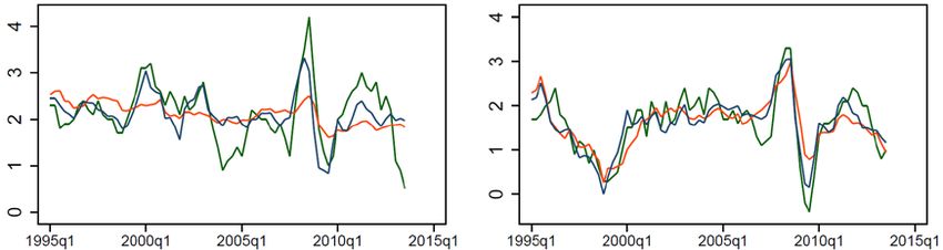
Abstract

Inflation dynamics in advanced countries have produced two consecutive puzzles during
the years after the global financial crisis. The first puzzle emerged when inflation rates
over the period 2009–11 were consistently higher than expected, although economic
slack in advanced countries reached its highest level in recent history. The second puzzle
– still present today – was initially observed in 2012, when inflation rates in advanced
countries were weakening rapidly despite the ongoing economic recovery. This paper
specifies a global Phillips curve for headline inflation using inflation expectations by
professional forecasters and a measure of economic slack at the global level over the
period 1995q1–2013q3. Phillips curve data points in the period after the global financial
crisis show a significantly different but consistent pattern compared to data points in the
period before or during the crisis. In the next step, potential explanatory variables at the
global level are assessed regarding their ability to improve the in-sample fit of the global
Phillips curve. The analysis yields three main findings. First, the standard determinants
can still explain a sizable share of global inflation dynamics. Second, household inflation
expectations are an important addition to the global Phillips curve. And third, the fiscal
policy stance helps explain global inflation dynamics. When taking all three findings into
account, it is possible to closely replicate global inflation dynamics over the post-crisis
period.

JEL classification: E31, E5, F41
Bank classification: Inflation and prices; International topics; Fiscal policy

                                        Résumé

La dynamique de l’inflation au sein des pays avancés a donné lieu à deux énigmes, qui se
sont succédé après la crise financière mondiale. La première apparaît au moment où, de
2009 à 2011, les taux d’inflation étaient systématiquement plus élevés que prévu tandis
que le niveau des capacités excédentaires atteignait, de mémoire récente, un sommet. La
seconde énigme persiste à ce jour : malgré la reprise, l’inflation connaît un
affaiblissement rapide pour la première fois en 2012. Dans son étude, l’auteur spécifie
tout d’abord une courbe de Phillips mondiale de l’inflation nominale en s’appuyant sur
les anticipations d’inflation de prévisionnistes professionnels, ainsi qu’une mesure des
capacités excédentaires à l’échelle internationale pour la période allant du
1er trimestre 1995 au 3e trimestre 2013. Après la crise, les points de données de la courbe
présentent une forme homogène sensiblement différente de la forme épousée avant ou
pendant la crise. L’auteur évalue ensuite l’aptitude de plusieurs variables explicatives à
améliorer l’adéquation statistique sur l’échantillon pour la spécification choisie de la
courbe de Phillips. De son analyse se dégagent trois conclusions importantes. 1) Les
déterminants habituels permettent encore d’interpréter une bonne partie de la dynamique
de l’inflation à l’échelle internationale. 2) Les anticipations d’inflation des ménages sont
un apport important à la courbe de Phillips mondiale. 3) L’orientation de la politique

                                             iii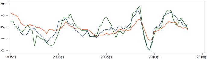
budgétaire aide à expliquer le comportement de l’inflation dans le monde. La prise en
compte de ces trois observations rend possible une reproduction plus fidèle de la
dynamique de l’inflation dans l’après-crise.

Classification JEL : E31, E5, F41
Classification de la Banque : Inflation et prix; Questions internationales; Politique
budgétaire

                                            iv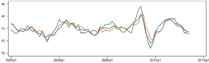
1        Introduction
Inflation dynamics in advanced countries have been largely puzzling over the recent past. While
inflation rates fell sharply during the global financial crisis and thus behaved as expected, their
subsequent post-crisis evolution is much harder to align with economic theory. In fact, two
distinct puzzles have emerged. The first puzzle is defined by the observation that inflation rates
over the period 2009-2011 were consistently higher than expected, even though economic slack
in advanced countries was at its highest level in recent history. The second puzzle emerged from
2012 onwards, when inflation rates in many advanced countries were weakening rapidly despite
the ongoing economic recovery.
    The first puzzle was initially raised by Williams (2010) in the context of the United States
and later expanded to advanced countries in general by WEO (2013). The puzzle concerns
the fact that inflation rates have remained very stable following the financial crisis – despite
rising levels of unemployment. The key explanatory factors cited in WEO (2013) were stable
inflation expectations arising from successfully established inflation-targeting regimes and a
long-term decline in the slope of the Phillips curve, i.e., an increasingly weaker sensitivity of
inflation to economic slack. The main conclusion of the analysis was that as long as central
bank independence was maintained, inflation would evolve around the inflation target.
    The second puzzle emerged more recently. During 2012, inflation rates in advanced coun-
tries suddenly started falling and have remained substantially below target since. In light of
these developments, the IMF has recently issued a warning about the risk of global deflation.1
Although most advanced economies still face substantial amounts of economic slack (especially
in Europe), it is specifically puzzling why the phenomenon of falling inflation rates occurs at a
time when economic slack in many countries is dissipating gradually.
    In this paper, I contribute to the literature by reconciling the two puzzles at the international
level and examining a broad set of common explanations for both. I start with the specifica-
tion of a global Phillips curve that explains the dynamics of headline inflation using inflation
expectations and a measure of economic slack at the global level over the 1995q1-2013q3 period.
It turns out that all the Phillips curve data points during the post-crisis period, defined as the
time after 2009q4, show a consistent but significantly different pattern than data points before
or during the crisis period. In the next step, a variety of potential explanatory variables are
assessed in terms of their ability to improve the in-sample fit of the Phillips curve. The analysis
yields three main findings. First, the standard determinants can explain a sizable share of global
inflation dynamics. Second, household inflation expectations are an important addition to the
global Phillips curve. Moreover, household inflation expectations appear to be more volatile
than inflation expectations by professional forecasters and most likely are a proxy for energy
and food price dynamics. And third, the government budget balance helps predict inflation dy-
namics as well. When all three findings are taken into account, it is possible to closely replicate
global inflation dynamics over the post-crisis period.
    While this paper explicitly deals with global inflation dynamics in the post-crisis period, it is
not the first one to examine global inflation. Although only a few papers specify a global Phillips
curve explicitly, there is a large body of academic literature that incorporates international
elements in domestic Phillips curves (see Eickmeier and Pijenburg (2013) and references cited
therein). The typical paper in this literature uses a standard Phillips curve framework and
augments it with international variables, such as import-price inflation and a global measure of
weighted (e.g., by GDP, Purchasing Power Parity (PPP), or trade) output gaps/unit labor costs.
    1
        See Lagarde (2014).

                                                 2
Although several authors find a statistically significant impact of these global determinants on
domestic inflation rates, the findings are often only marginally significant and usually not very
robust to the sample selection.2
Papers that study global inflation dynamics more explicitly are Ciccarelli and Mojon (2005),
Hakkio (2009), Monacelli and Sala (2009), and Mumtaz and Surico (2012).3 The findings of this
smaller body of literature indicate that common components of industrial production, unem-
ployment rates, nominal wages, short- and long-term interest rates, the yield curve, and money
aggregates may be important determinants. Longer-term trends, such as sectoral trade open-
ness, have also been associated with the common elements of inflation. However, none of the
above papers discusses inflation dynamics in the post-crisis years.
The remainder of the paper is organized as follows. Section 2 defines the two inflation puz-
zles and characterizes global inflation dynamics. Section 3 contains the core of the paper and
consists of three subsections. The first sets up a global Phillips curve and explains that standard
determinants are not able to sufficiently account for global inflation dynamics in the post-crisis
period. A second subsection discusses a list of variables that could potentially explain the weak
post-crisis fit, and a third subsection identifies those variables from the list that yield the best
statistical fit. Section 4 then provides an interpretation of the findings and examines their ro-
bustness. Finally, Section 5 concludes.
2 Characterizing Global Inflation Dynamics
2.1 Defining the Two Inflation Puzzles
The first inflation puzzle was initially raised in the U.S. context. As pointed out in the in-
troductions of Ball and Mazumder (2011) and Gordon (2013), the first reference to a “missing
deflation puzzle” dates back to Williams (2010), who mentioned in a public speech that, “based
on the experience of past severe recessions,” he would have expected “inflation to fall by twice
as much as it has”. Subsequently, several authors took up the puzzle notion and tried to pro-
vide an empirical explanation for its occurrence – most of them used a version of the U.S.
Phillips curve as the underlying tool. Ball and Mazumder (2011) provide two modifications
of the Phillips curve. First, the authors measure core inflation with the weighted median of
consumer price inflation across industries, and second, they allow the slope of the Phillips curve
to change with the level and variance of inflation. Murphy (2014) discusses a similar line of ar-
guments and suggests that the time-varying slope of the Phillips curve is driven by sticky-price
and sticky-information approaches to price adjustments. By including a measure of uncertainty
about regional economic conditions, Murphy argues that the recent path of inflation is explained
well. A different approach is taken by Gordon (2013) who uses the “triangle model” from the
early 1980s to explain away the missing deflation puzzle for the United States. The triangle
model expresses current U.S. inflation with backward-looking inflation expectations, a measure
of economic slack to capture demand-side developments and a measure of energy-price shocks to
account for supply-side dynamics. When the model is estimated from the early 1960s to 1996,
it predicts the U.S. inflation rate in 2013q1 within 0.5 percentage points – without changing the
2
In a very recent paper, Medel et al. (2014) study the information content of global inflation dynamics for the
prediction of national inflation rates in 31 countries. Their findings indicate that, especially in recent years, there
is predictive content contained in the international inflation measure, but its impact on national inflation rates is
very heterogeneous.
3
Table A1 in the Appendix shows a more detailed description of these papers.
3slope of the Phillips curve over time. Gordon also argues that the predictions improve when
the (total) unemployment rate is replaced by an explicit measure for short-term unemployment.
Finally, Coibion and Gorodnichenko (2013) discuss the absence of disinflation dynamics in the
United States over the years 2009-2011. By using household inflation expectations as a measure
of inflation expectations in the Phillips curve, the authors manage to re-establish the Phillips
curve relationship for the United States since the 1960s.
The theoretical literature has also discussed potential explanations for the first puzzle. The
performance of DSGE models in describing inflation dynamics over the global financial crisis
and the early post-crisis period has been criticized by Hall (2011) and King and Watson (2012).
Del Negro et al. (2014) challenge these critiques by including financial frictions in a standard
DSGE model. The resulting model predicts a sharp contradiction in economic activity, along
with a modest and protracted decline in inflation following the period of financial stress at the
end of 2008. In addition, Gilchrist et al. (2013) provide evidence for a channel leading from firm
balance sheets to inflation dynamics. The authors demonstrate that firms with “weak” balance
sheets increase their prices significantly in order to generate required revenues, and firms with
strong balance sheets lower their prices in order to maintain their customer base. This finding
helps explain inflation dynamics in the United States during the crisis itself, as well as during the
early post-crisis period. Finally, Christiano et al. (2014) examine the dynamics of a broad set of
economic variables in the United States over the crisis and the post-crisis period. The authors
identify four shocks that can describe the features of the data well: a consumption wedge to
proxy the zero lower bound, a financial wedge to describe credit market frictions, a technology
shock that captures the decline of total factor productivity, and a government consumption
shock. The authors conclude that the fall in total factor productivity and the rise in the cost of
working capital were important factors that kept U.S. inflation high over the crisis.
The generalization of the first puzzle to the international level was then undertaken in WEO
(2013). Here, it was observed that inflation rates in advanced countries remained very stable fol-
lowing the financial crisis despite continuously rising unemployment rates. The key explanatory
factors cited were stable inflation expectations arising from successfully established inflation-
targeting regimes and a long-term decline in the slope of the Phillips curve, i.e., an increasingly
weaker sensitivity of inflation to economic slack. The main conclusion of the chapter is that as
long as central bank independence is maintained, inflation will evolve around the target.
Figure 1 documents the presence of the first puzzle for a broad set of advanced countries.
The bars indicate the deviation of quarterly headline inflation – measured on a year-on-year
basis – from the mean value of the implicit or explicit inflation target of the associated central
bank. The blue bars describe the deviation of the average inflation rate over the period 2009q4-
2011q4. It turns out that all countries, with the exception of Switzerland, Japan and Ireland,
have exhibited positive or only slightly negative deviations from the target during the first part
of the post-crisis period. Figure 1 also shows that at the beginning of the first puzzle period
(i.e., in 2009), annual real GDP growth across all sample countries amounted to 3.58%. Hence,
above-target inflation rates occurred at a time when economic growth was at its lowest level in
recent history and one would rather expect deflationary pressures to occur.
The second puzzle emerged more recently. From 2012 onwards, inflation rates in the same
set of advanced countries suddenly started falling and have remained substantially below target
since. This development is indicated by the red bars that show the deviation of average inflation
from target for the period 2012q1-2013q3. It turns out that most countries have experienced
a clearly negative deviation over the second part of the post-crisis period. Although most ad-
4Figure 1: Illustration of the Two Puzzles
3 p.p.
Average Annual Real GDP Growth:
in 2009: -3.58 %
in 2012: 0.35 %
Avg. Deviation of Inflation from Target
2
1
0
-1
-2
Puzzle 1: 2009q4-2011q4 Puzzle 2: 2012q1-2013q3
-3
Note: Inflation targeters enter with the center of their target. The targets are 2% in all cases but the following ones: Australia
(2.5%), Iceland (2.5%), Korea (3%), and Norway (2.5%). The average deviation is calculated for each of the two subsamples
separately.
vanced economies still face substantial amounts of economic slack (especially in Europe), it is
specifically puzzling why the phenomenon of falling inflation rates occurs at a time when the
economic recovery had set in and economic slack is gradually dissipating in a large number of
countries. Figure 1 shows that at the beginning of the second puzzle period (i.e., in 2012), annual
real GDP growth across all sample countries amounted to 0.35%. Although highly discussed
in policy circles, this puzzle has not yet received much attention in the academic literature.
The most closely related papers are Svensson (2013) and Ferroni and Mojon (2014). Svensson
(2013) describes a similar experience for the case in Sweden, where inflation rates have been
below target since 1997. He argues that keeping inflation rates below target for an extended
period of time results in a 0.8 percentage point higher unemployment rate in Sweden over the
period 1997-2011. Ferroni and Mojon (2014) examine the predictive content of global inflation
for domestic inflation with a sample ranging until 2013. Using a variety of potential forecasting
models, the authors find that this is indeed the case. In the next step, the authors try to identify
the underlying forces at both the domestic and the global levels by specifying a VAR with sign
restrictions that identify two domestic (supply and demand) and two global shocks (commodity
prices and world demand). The authors specifically find that global supply-side factors, e.g.,
commodity prices, are most likely not the main driver of inflation dynamics after 2009. Instead,
the authors argue that falling inflation rates in 2008-2009, and during the second puzzle period,
are caused by demand shocks – with relative contributions of global and domestic shocks varying
by country and time.
Finally, to sum up the findings from the literature and the evidence from Figure 1, it can be
seen that both inflation puzzles appear in a broad set of advanced countries and seem to be even
stronger for countries other than the United States. Therefore, the next subsection combines
the information contained in national inflation rates to construct a “global” inflation rate.
52.2 Constructing Measures of Global Inflation
“Global” inflation dynamics in this paper are based on national inflation data from 25 advanced
countries over the period from 1995q1 to 2013q3.4 National inflation rates are obtained by
computing year-on-year growth rates of the individual Consumer Price Index (CPI) for each
country. The data are obtained from the OECD and come in quarterly frequency. Global
inflation rates are shown separately for headline and core inflation, where core inflation is defined
as headline inflation purged of food and energy prices. Largely based on Ciccarelli and Mojon
(2005), I use the following three methods to identify global inflation:
• A static factor model: The first approach here is the standard approach in the literature.
It relies on the first common factor of national inflation rates. The underlying (static)
factor model can be written as:
Xi,t = Λk,i × Fk,t + Ui,t (1)
Equation (1) expresses national inflation rates (Xi,t ) in terms of a set of orthogonal vari-
ables, the common factors (Fk,t ), with k = 1, 2, ..., K. I extract the resulting variable that
captures the largest common variation, the first common factor F1,t . The factor model
also produces factor loadings Λk,i , which range from 0 to 1, and quantify the importance
of the first common factor for each country. Finally, Ui,t represents the country-specific or
idiosyncratic part of the variation in Xi,t , which cannot be explained by the first common
factor. National inflation rates are standardized by subtracting their individual mean and
dividing by their standard deviation before entering the factor model.
• An unweighted average: The second approach is based on the unweighted arithmetic
mean of all national inflation rates. For comparison purposes with the factor model, the
resulting global inflation series is standardized as well.
• A PPP weighted average: Finally, the third approach is based on a weighted arith-
metic mean of national inflation rates, where the weights constitute world PPP shares
(normalized to 1 among all sample countries) obtained from the WEO database. Again,
the resulting global inflation series is standardized by subtracting the mean and dividing
by its standard deviation.
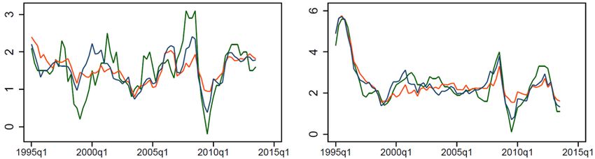
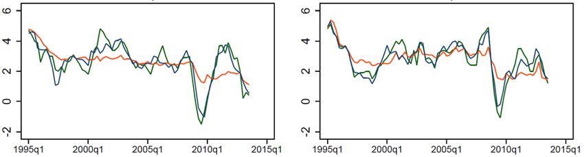
Figure 2 shows the results. The global inflation rates obtained using any of the three ap-
proaches are very similar. The following observations emerge: First, headline inflation is more
volatile than core inflation (note the different scales in the two plots), especially during the ac-
tual crisis period. Second – in line with the first puzzle – the period 2009-2011 shows a sustained
upward movement in both inflation concepts. Third – in line with the second puzzle – more
recently, all measures of global inflation show a clear downward trend.
The remainder of this paper deals with the specification of a global Phillips curve based on
global headline inflation and the factor approach as the aggregation technique.5 In order to
explain global inflation dynamics with global determinants, all potential explanatory variables
4
I hereby follow the convention of the literature to use the “global” terminology but keeping the focus on
advanced countries only (see Ciccarelli and Mojon (2005) for example). The sample countries correspond to
the ones presented in Figure 1 and comprise Australia, Austria, Belgium, Canada, Denmark, Finland, France,
Germany, Greece, Iceland, Ireland, Israel, Italy, Japan, Korea, Luxembourg, Netherlands, New Zealand, Norway,
Portugal, Spain, Sweden, Switzerland, the United Kingdom and the United States.
5
The robustness of the results to alternative aggregation techniques is examined in Section 4.2.
64
Figure 2: Global Headline (left) and Core (right) Inflation
3
2
2
1
0
0
-2
-1
-2
-4
1995q1 2000q1 2005q1 2010q1 2015q1 1995q1 2000q1 2005q1 2010q1 2015q1
Date Date
Headline Inflation, 1st Factor Headline Inflation, unw. Avg. Core Inflation, 1st Factor Core Inflation, unw. Avg.
Headline Inflation, w. Avg. Core Inflation, w. Avg.
are aggregated from the national to the global level using the same methods as shown above.
However, not all potential explanatory variables are available for the full set of sample countries
and, with only a very few exceptions, I include only those national variables in the aggregation
process that cover the entire sample period.6
3 Specifying a Global Phillips Curve
The goal of this section is to specify a global Phillips curve and specifically examine the impact
of the crisis on its structure. The first subsection presents the shape of the standard Phillips
curve before, during and after the crisis and discusses the relationship between the previously
identified puzzles. The second subsection presents a large set of potential explanations for the
puzzles and introduces a strategy to test for the most likely one(s). Finally, the third subsection
discusses the outcome of the tests and specifies an augmented global Phillips curve.
3.1 The Global Phillips Curve with Standard Determinants
Following the identification of a global inflation rate in Section 2.2, this subsection aims to
explain global inflation using standard determinants from the literature. In order to specify
a global Phillips curve for global headline inflation, I largely follow the steps of Coibion and
Gorodnichenko (2013) who specify a Phillips curve in the U.S. context. First, I calculate a mea-
sure of global “surprise” inflation that is obtained by subtracting global inflation expectations
from the previously obtained global headline inflation series based on the first common factor.
The global measure of inflation expectations is derived in the exact same way and is based on
national series of inflation expectations by professional forecasters for the next calendar year,
provided by Consensus Economics. Second, as a measure of economic slack, I calculate a global
unemployment rate – again based on the first factor of national unemployment rates. Finally, I
plot both variables in a scatter plot with the inflation surprise measure on the vertical and the
measure of economic slack on the horizontal axis.
6
Appendix Table A2 presents the exact country composition that underlies each of the global determinants.
7Figure 3: The Global Phillips Curve I
2
2001q2
2008q2
2008q1 2008q3
2001q1 2011q2
2003q1
2011q1
2011q32011q4
1
2007q4 2001q3
2000q3 2005q3 2012q1
2006q2
2003q3
2001q4 2002q4 2004q4 2010q4
2000q4
2002q1 2003q2
2003q4
2008q4 2005q1
2000q2 2005q2
2004q2
2005q4 2004q3
2006q1
Surprise Inflation
2000q1 2010q2
2006q3 2010q3
2012q3
2007q1 2002q3 1999q4 2012q2 2012q4
0
2007q2 2010q1
2002q2
2009q1
2006q4
2007q3
1999q3 2009q4
2004q1 1999q2 2013q3
1998q4 1996q4
2009q2
2013q1
1999q1 2013q2
-1
1996q3
1998q31998q2 1997q4
1997q3 1996q2
2009q3
1997q1
1998q1 1995q4
1997q2
1996q1
-2
1995q2
1995q1
1995q3
-2 -1 0 1 2
Unemployment Rate, 1st Factor
Note: Surprise Inflation = Difference between the 1st factor of headline inflation and the 1st factor of inflation expectations by
professional forecasters for the next calendar year.
Figure 4: The Global Phillips Curve II
2
2001q2
2008q2
2008q3 2008q1
2011q2 2001q1
2003q1
2011q1
2011q3
2011q4
1
2001q3 2007q4
2012q1 2005q3 2000q3
2006q2
2010q4 2003q3 2004q4
2002q4 2001q4 2000q4
2003q4 2003q2 2002q1
2004q2 2005q2
2005q1 2000q2 2008q4
2005q42006q1
Surprise Inflation
2004q3
2010q2 2000q1
2010q3 2006q3
2012q3
2012q4 2012q2 1999q4
2002q3 2007q1
0
2010q1 2007q2
2002q2
2009q1
2006q4
2007q3
2009q4 1999q3
2013q3 2004q1 1999q2
1996q4 1998q4
2009q2
2013q1
2013q2 1999q1
-1
1996q3
1998q2
1997q4 1998q3
1996q2 1997q3
2009q3
1997q1
1995q4 1998q1
1997q2
1996q1
-2
1995q2
1995q1
1995q3
-2 -1 0 1 2
OECD Output Gap, 1st Factor
Note: Surprise Inflation = Difference between the 1st factor of headline inflation and the 1st factor of inflation expectations by
professional forecasters for the next calendar year.
8Based on Figure 3, which shows the results, we can make the following observations:
• First, there is a negative long-run relationship between the two variables during the pre-
crisis period from 1995q1 to 2007q3 (blue line).
• Second, the relationship in the crisis period is fairly similar to the pre-crisis period between
2007q4 and 2009q3 (green line).
• And third, most importantly, the entire post-crisis period, 2009q4-2013q3, shows a signif-
icantly different, but consistent, pattern with a steeper slope and a higher intercept term
(red line).
The third observation in particular requires a more detailed discussion. Evidence so far has
suggested that there are two distinct puzzles at work, one with inflation rates for the period
2009-2011 that are too high and one with inflation rates from 2012 onwards that are too low.
However, Figure 3 now reveals that surprise inflation in the entire post-crisis period is consis-
tently more sensitive to changes in economic slack and consistently higher for reasons unrelated
to economic slack. Hence, the two puzzles discussed so far can be combined into a single one,
which I henceforth term the “Twin Puzzle.” Using the unemployment rate as a measure of
economic slack has the advantage that data are available at a quarterly frequency. However,
since the Phillips curve is mostly specified using an output gap, Figure 4 shows the same rela-
tionship using the output gap as the measure of economic slack. While the result confirms the
findings in Figure 3 (this time with a prior for a positive slope), the output gap measure has
a major drawback. As output gap data for most of the sample countries are available only at
annual frequency, the data have to be linearly interpolated to a quarterly frequency. Hence, the
observations align more closely around the regression lines, suggesting an even better fit.
Next, we can use the above findings to specify an econometric model for global inflation.
The starting point is a simple Phillips curve equation that corresponds to Figure 3. By moving
inflation expectations to the right-hand side and assigning the coefficient β, global headline
inflation (πt ) is expressed in Equation (2) in terms of global inflation expectations (πte ), and the
global unemployment rate (unempt ). Finally, εt represents an error term.
πt = α + βπte + γunempt + εt (2)
Specification 1 in Table 1 shows the estimated coefficients of the baseline specification, and
Figure 5 illustrates the resulting in-sample fit. As already expected from observing Figure
3, the standard Phillips curve relationship – containing inflation expectations by professional
forecasters (PFC) and the unemployment rate – does not do very well in predicting inflation
during the post-crisis period. When examining Figure 5 more closely, however, it turns out
that the in-sample prediction does a fairly good job in capturing the higher-frequency dynamics
during this period. The only problem seems to be a level and a scaling difference from around
2009 onwards. Equation (3) therefore introduces a Post-Crisis Dummy (Dpct ) that takes on the
value of 1 during the period 2009q4-2013q3 and 0 elsewhere:
πt = α + βπte + γunempt + ψDpct + δπte × Dpct + θunempt × Dpct + εt (3)
9Table 1: The Baseline Specification With and Without Post-Crisis Dummy
Dependent Variable:
(1) (2) (3) (4) (5)
Headline Inflation
Unemployment Rate -0.54*** -0.64*** -0.96*** -0.95*** -0.93***
(0.00) 0 (0.00) (0.00) (0.00)
Inflation Expectations by PFC, next year 0.71*** 1.00 1.01*** 1.00 0.97***
(0.00) (.) (0.00) (.) (0.00)
Post-Crisis Dummy 2.99*** 2.98*** 3.32***
(0.00) (0.00) (0.00)
Unemployment Rate x Post-Crisis Dummy -1.47*** -1.48*** -1.54***
(0.00) (0.00) (0.00)
Infl. Exp. By PFC x Post-Crisis Dummy 0.68***
(0.00)
Observations 75 75 75 75 75
R-squared 0.52 0.78 0.80
Note: P-Values in parentheses. Constant not reported. The stars indicate significance levels (also in all subsequent tables):
*** pFigure 6: In-Sample Fit With a Post-Crisis Dummy
4
2
0
-2
-4
1995q1 2000q1 2005q1 2010q1 2015q1
Date
Actual Inflation Baseline with Post-Crisis Dummy
Note: Actual Inflation = 1st factor of headline inflation. Baseline Specification = In-sample fit for the
standard global Phillips curve specification, containing the unemployment rate and inflation expec-
tations by professional forecasters. Post-Crisis Dummy = Level and interaction terms of a dummy
taking on the value of 1 over 2009q4-2013q3.
confirmed here that adding and interacting the post-crisis dummy with the standard Phillips
curve determinants remarkably improves the in-sample fit over the post-crisis period. Finally,
Specifications 2 and 4 in Table 1 show that the results are fairly similar when constraining the
coefficient on inflation expectations, β, to be equal to 1 (as was implicitly the case in Figure
3). Especially when looking at Specification 3, it turns out that inflation expectations receive a
coefficient close to 1, even in the unconstrained case.
Before moving on and testing which variable(s) could be underlying the post-crisis dummy, it
is helpful to conduct a historical decomposition for the determinants contained in Specification
5. The contributions of the individual determinants are calculated by combining the estimated
coefficients with the values of the underlying variables at each point in time. Figure 7 shows the
result. Inflation expectations by professional forecasters played the most important role in the
second half of the 1990s. The introduction of inflation targeting made agents and, hence, also
professional forecasters revise their inflation expectations downward. On the other hand, global
inflation dynamics in the 2000s were mostly driven by contributions of the unemployment rate.
The crisis itself was then characterized by falling inflation expectations, while unemployment
had not fully reacted yet. However, this changes significantly in the post-crisis period. Whereas
inflation expectations by professional forecasters play a key role from mid-2009 to 2011, most of
the post-crisis period is driven by a different variable. The high importance of the interaction
term between the crisis dummy and the unemployment rate suggests that the effect is closely
related to economic slack – however, it could also proxy for crisis-related dynamics in other vari-
ables. Finally, Figure 7 shows that the post-crisis dummy has shifted inflation in the post-crisis
period up by a significant amount.
114
2
0
-2
-4 Figure 7: Contributions of Individual Determinants – Post-Crisis Dummy
Post-Crisis Dummy PFC Infl. Exp.
PFC Exp. Interaction Unemp. Rate
Unemp. Interaction Constant
Residual
-6
1995q1 2000q1 2005q1 2010q1 2013q3
3.2 Potential Explanatory Variables to Augment the Global Phillips Curve
The previous subsection has shown that adding a post-crisis dummy to the standard Phillips
curve specification significantly improves the fit during the entire period. The goal of this subsec-
tion is to give an economic meaning to the post-crisis dummy and to determine if it potentially
proxies for another variable. Since the crisis and the post-crisis periods brought a substantial
number of structural changes, the list of potential explanatory variables is long. In order to
structure the analysis, I group them in the following five categories: additional measures of
inflation expectations, additional measures of economic slack, policies and policy uncertainty,
commodity prices, and financial variables. Table 2 shows all candidate variables and their place-
ment into the categories.7
(i) Additional Measures of Inflation Expectations: Inflation expectations differ pri-
marily along the following two dimensions:
• forecasting entity (i.e., surveys among professional forecasters, surveys among households,
or expectations calculated from financial market data); and
• forecasting horizon (e.g., next calendar year or 1, 5, 10 years ahead). In general, we expect
that inflation expectations generated by professional forecasters over the longer term are
closer to central bank targets, and that inflation expectations by households over the short
term are more affected by current inflation rates.
7
Summary statistics are shown in Table A3 in the Appendix.
12The role of household inflation expectations is of particular interest in the context of the global
Phillips curve. Coibion and Gorodnichenko (2013) suggest that household inflation expectations
are good proxies for inflation forecasts by small firms. The authors argue that using these ex-
pectations yields a stable Phillips curve relationship for the United States and therefore solves
the first part of the post-crisis puzzle (i.e., inflation dynamics during 2009-2011). Unfortunately,
there is no internationally consistent series for inflation expectations by households. I therefore
use data from two different sources and treat each of them as separate variables.8 Expectations
by households appear to be more volatile, especially in the United States, and are also more
elevated compared with inflation expectations by professional forecasters – even more so during
the post-crisis period.
(ii) Additional Measures of Economic Slack: Owing to the annual frequency of in-
ternational output gap measures, this paper relies primarily on the unemployment rate as the
measure of economic slack in the Phillips curve. Under certain assumptions, output gaps and
unemployment gaps can be used interchangeably. However, in the presence of a jobless recovery
or prolonged periods of slack, traditionally measured output gaps may not align well with un-
employment gaps. Further, additional measures of economic slack, such as labor compensation
measures or unit labor costs, might become more important in times of crises.
(iii) Policies and Policy Uncertainty: The global financial crisis was followed by an
unprecedented amount of fiscal and monetary easing, possibly raising uncertainty.
• Fiscal Policy: In this paper, fiscal policy is represented by the variable Net Lending/Bor-
rowing of the General Government in % of GDP, henceforth referred to as the “government
budget balance.” Economic theory suggests that fiscal policy affects inflation dynamics
through the measure of economic slack. However, in the presence of a deep and prolonged
recession, this standard relationship could change, and large government budget deficits
could have an additional direct effect on inflation, over and above the unemployment
rate/output gap measure.
• Unconventional Monetary Policy: The adoption of unconventional monetary policies could
lead to price increases, not only in asset markets but also in goods markets.
• Inflation Expectation Uncertainty: Inflation expectations from professional forecasters
usually refer to the next calendar year. One could therefore expect an improvement in the
forecasts towards the end of the year.
(iv) Commodity Prices: Although the previous literature has shown that inflation expec-
tations, especially by households, are highly correlated with commodity-price dynamics (with a
lag), the additional inclusion of energy and food prices in the Phillips curve might improve the
fit – even more so when inflation expectations are focused on the long term.
(v) Financial Variables: A number of theoretical papers discuss the impact of financial
frictions (e.g., Christiano et al., 2014; Del Negro et al., 2014) and firm balance sheets (e.g.,
8
Inflation expectations by U.S. households are from the Michigan Survey of Consumers and are based on the
question: “By about what percent per year do you expect prices to go up or down, on the average, during the
next 12 months?” Inflation expectations by European households are provided by the OECD for 11 countries in
our sample and are based on the question: “By comparison with the past 12 months, how do you expect that
consumer prices will develop in the next 12 months?” Possible answers range from “increase more rapidly” to
“fall” in five steps and are converted into an overall index.
13Table 2: Description of Potential Explanatory Variables
# Category/Variable Description Source
Inflation Expectations
BL Professional Forecasters, next Inflation expectations by professional forecasters for the next calendar year Consensus
calendar year Economics
1 Headline Inflation, backward- Average of headline inflation during the last 4 quarters OECD, BoC
looking Calculations
2 Core Inflation, backward-looking Average of core inflation over the last 4 quarters OECD, BoC
Calculations
3 US Households, 1 year-ahead Inflation expectations by US households based on the question: "By what Surveys of
percent do you expect prices to go up, on the average, during the next 12 Consumers, Univ. of
months?" Michigan
4 US Households, 5+ years-ahead Inflation expectations by US households based on the question: "By about Surveys of
what percent per year do you expect prices to go up or down, on the average, Consumers, Univ. of
during the next 5 to 10 years?" Michigan
5 European Households, 1 year- Index for inflation expectations by European households based on the OECD
ahead question "By comparison with the past 12 months, how do you expect that
consumer prices will develop in the next 12 months?" Possible answers range
from "increase more rapidly" to "fall" in 5 steps.
6 Professional Forecasters, 5 Inflation Expectations by Professional Forecasters in 5 Years Consensus
calendar years from now Economics
7 Professional Forecasters, 10 Inflation Expectations by Professional Forecasters in 10 Years Consensus
calendar years from now Economics
8 Market-based, over the next 5 Difference between yields of inflation-indexed bonds and non-indexed bonds Bloomberg, BoC
years Calculations
9 Market-based, over the next 10+ Difference between yields of inflation-indexed bonds and non-indexed bonds Bloomberg, BoC
years Calculations
Measures of Economcic Slack
BL Unemployment Rate The unemployment rate in percent OECD
10 Output Gap Interpolated quarterly values of annual output gap estimates from the OECD OECD
11 Unemployment Gap Cyclical component of the unemployment rate, obtained using an HP filter
OECD, BoC Calc.
12 Real GDP Gap Cyclical component of a real GDP index, obtained using an HP filter OECD, BoC Calc.
13 Industry Production Gap Cyclical component of an industry production index, obtained using an HP
OECD, BoC Calc.
filter
14 Industry Production Growth YoY growth rate of an industry production index OECD
15 Unit Labor Cost Growth YoY growth rate of an index of unit labor costs OECD
16 Labor Compensation Growth YoY growth rate of an index of labor compensation OECD
Policies and Policy Uncertainty
17 Gov. Budget Balance General government net lending/borrowing in % of GDP, interpolated to IMF
quarterly frequency
18 Growth of QE-Quantities Growth of QE quantities in % of GDP; in levels for Figure 7C, in growth rates Dahlhaus, Hess,
for the empirical analysis. Reza (2014)
19 Inflation Expectations Uncertainty Standard deviation across the individual mean forecasts/inflation Consensus
expectations by professional forecasters in the next calendar year (first Economics
variable in the list)
Commodity Prices
20 Oil Price YoY growth rate of Brent Index. Intercontinental
Exchange
21 Energy Prices YoY growth rate of energy prices IMF
22 Food Prices YoY growth rate of food prices IMF
Financial Variables
23 Financial Market Uncertainty VIX Index Chicago Board
Options Exchange
(CBOE)
24 Credit Growth YoY growth rate of credit to private non-fianncial sector in % of GDP BIS
25 Stockmarket Growth YoY growth rate of the MSCI World index Bloomberg
26 Real Estate Price Growth YoY growth rate of a real estate index (res. property, all dwellings) BIS
BL = Baseline Specification
14Gilchrist et al., 2013) on output and inflation dynamics during the global financial crisis. In ad-
dition, Borio et al. (2013) have recently shown empirically that accounting for cyclical financial
variables can improve the estimation of potential output and the output gap. Hence, financial
variables could indeed be important drivers of inflation dynamics. I therefore examine the role
of stock market prices, real estate prices and private credit in helping to predict global inflation.
In addition, the VIX index is also tested, since uncertainty about financial developments could
be an important driver of global inflation dynamics.
3.3 What Explains the Twin Puzzle at the Global Level?
To better understand the shift in inflation dynamics, I begin by estimating the baseline spec-
ification, which contains the unemployment rate and inflation expectations from professional
forecasters for the next calendar year (results were shown in Specification 1 of Table 1). I then
re-estimate the model with the addition of each of the 26 potential explanatory variables listed in
Table 2 to optimally match the structural shift during the post-crisis period observed in Figure
3. The corresponding functional form for the analysis is given by Equation (4):
πt = α + βπte + γunempt + ψV arXt + δπte × V arXt + θunempt × V arXt + εt (4)
where V arXt is the variable to be tested as a potential determinant that could be responsible
for the post-crisis level and slope shift. Hence, each candidate variable is included as it is, as an
interaction term with the unemployment rate and as an interaction term with the expectations
by professional forecasters. The resulting specifications are evaluated using the (lowest) Mean
Squared Error (MSE) for the following four intervals:9
• the entire sample period (1995q1-2013q3);
• the entire post-crisis period (2009q4-2013q3);
• the period of the first puzzle (2009q4-2011q4); and
• the period of the second puzzle (2012q1-2013q3).
Table 3 shows the results. The potential explanatory variables are ordered according to the
MSEs of their underlying specifications over the entire sample period from the lowest to the
highest.10 The variable with the lowest MSE of all the candidate variables is the measure of
inflation expectations by European households over the next 12 months (MSE of 0.50). Inter-
estingly, this variable is followed by a measure of inflation expectations by U.S. households over
the same time frame (MSE of 0.55). The variables that follow this selection in turn are the
growth rates of real estate prices (MSE of 0.56), as well as the growth rates of food and energy
prices (both have an MSE of 0.57).
9
As some of the intervals are very short, the MSE is calculated without a degree of freedom adjustment. This
overstates the MSE in absolute terms but it does not affect its ordering as in all cases the same number of variables
is included in the regression
10
In the remainder of this section, the MSE associated with each variable refers to the MSE of the underlying
specification including this variable; i.e., the baseline specification plus the variable under examination.
15Table 3: Potential Explanatory Variables Ordered by Mean Squared Error
Variable added 1995q1-2013q3 2009q4-2013q3 2009q4-2011q4 2012q1-2013q3
Infl. Exp. European Households, 1 year-ahead 0.50 0.43 0.52 0.29
Infl. Exp. US Households, 1 year-ahead 0.55 0.68 0.78 0.52
Real Estate Price Growth 0.56 0.79 0.89 0.63
Growth Rate of Food Prices 0.57 0.76 0.76 0.76
Growth Rate of Energy Prices 0.57 0.75 0.80 0.67
Real GDP Gap 0.58 0.60 0.75 0.31
Industry Production Gap 0.58 0.60 0.70 0.42
Growth Rate of Oil Price 0.59 0.77 0.83 0.70
Government Budget Balance 0.60 0.78 0.83 0.70
Unit Labor Cost Growth 0.60 0.87 1.03 0.60
Infl. Exp. for Core Inflation, backward-looking 0.60 0.73 0.72 0.74
Industry Production Growth 0.60 0.77 0.93 0.50
Output Gap 0.60 0.90 1.04 0.66
Credit Growth 0.60 0.83 1.02 0.48
Stock Market Growth 0.60 0.87 1.08 0.51
QE-Quantities 0.62 0.84 1.00 0.51
Infl. Exp. by Professional Forecasters, 5 years from now 0.63 0.80 0.90 0.66
Labor Compensation Growth 0.63 0.75 0.89 0.51
Infl. Exp. by Financial Markets, over the next 5 years 0.64 0.75 0.93 0.42
Infl. Exp. by US Households, 5+ years-ahead 0.64 0.73 0.89 0.44
Infl. Exp. by Professional Forecasters, 10 years from now 0.64 0.83 0.98 0.59
Financial Market Uncertainty 0.65 0.88 1.06 0.56
Unemployment Gap 0.65 0.84 1.01 0.53
Inflation Expectations Uncertainty 0.65 0.90 1.07 0.62
Infl. Exp. for Headline Inflation, backward-looking 0.66 0.90 1.10 0.55
Infl. Exp. by Financial Markets, over the next 10+ years 0.66 0.85 1.01 0.58
Memorandum
Baseline 0.69 0.93 1.11 0.62
Table 4: Derivation of the Augmented Baseline Specification
Dependent Variable:
(1) (2) (3) (4)
Headline Inflation
Unemployment Rate -0.37*** -0.33*** -0.91*** -0.75***
(0.00) (0.00) (0.00) (0.00)
Inflation Expectations by PFC, next year 0.30*** 0.34*** 0.51*** 0.47***
(0.00) (0.00) (0.00) (0.00)
Inflation Expectations by HH, 12 months 0.64*** 0.58*** 0.54*** 0.49***
(0.00) (0.00) (0.00) (0.00)
Unemp. Rate x Infl. Exp. by HH 0.12
(0.12)
Infl. Exp. By PFC x Infl. Exp. by HH 0.07
(0.23)
Budget Bal. in % of GDP -0.61*** -0.50***
(0.00) (0.00)
GR of World Energy Prices 0.70***
(0.00)
Observations 75 75 75 75
R-squared 0.75 0.74 0.82 0.86
Note: P-Values in Parentheses. Constant not reported.
16When looking at the (entire) post-crisis period, the MSE-reducing effect of household infla-
tion expectations becomes even more pronounced. Over the entire post-crisis sample, inflation
expectations by European households reach an MSE of 0.43, while the next variables, two mea-
sures of economic slack, reach an MSE of 0.6. The effect clearly originates from the first part
of the post-crisis period: while European household inflation expectations have an MSE of 0.52
here, the next variable reaches an MSE of 0.70 during 2009q4 and 2011q4. U.S. household
inflation expectations show a slightly higher MSE but still score fourth highest among all the
potential explanatory variables in the entire crisis period (MSE of 0.68), as well as sixth highest
(MSE of 0.78) in the first part of the post-crisis period. European household inflation expecta-
tions still dominate the list of potential explanatory variables in the second part of the post-crisis
period (MSE of 0.29); however, the difference with respect to the next candidate variable be-
comes smaller (the real GDP gap with an MSE of 0.31). Given their high but relatively constant
trajectory, U.S. household inflation expectations over the next 12 months have a higher MSE
now and score relatively lower among all potential explanatory variables (MSE of 0.52). In-
terestingly, the measure of U.S. household inflation expectations 5 years ahead turns out to be
better during this period. It ranks fifth among all the candidate variables and reaches an MSE
of 0.44.
Specifications 1 and 2 in Table 4 present the results after European household inflation ex-
pectations have been added to the baseline specification. There are two ways in which European
household expectations can be included in the specification. First, by adding the two interac-
tion terms as originally shown in Equation (4) and represented by Specification 1. Since it turns
out that abstracting from both interaction terms yields only a marginally lower fit, the second
approach, as shown in Specification 2, is to add only the level term to the baseline specification.
Figure 8 plots the corresponding in-sample fit and indicates that there is only a small dif-
ference between the two approaches. Finally, the figure also includes actual global inflation for
comparison. Although the two models that include household expectations show a similar in-
sample fit, they are less precise around the peak of global inflation during the post-crisis period.
The next section will therefore examine whether there is another variable that can account for
the higher inflation trajectory during the period in question.
In addition to European household inflation expectations, Figure A1 in the Appendix repli-
cates the analysis for U.S. household inflation expectations – the variable that had the second-
lowest MSE in Table 3 (see Specifications 1 and 2 in Appendix Table A4 for details). As expected
from the MSE, the in-sample fit of U.S. household inflation expectations is lower. Although the
in-sample prediction mirrors the spike in inflation rates during the post-crisis period, there still
seems to be a scaling difference. In addition, U.S. household inflation expectations have re-
mained largely constant over the post-crisis period, yielding an overprediction of inflation rates
at the end of the period.
The analysis so far has shown that household inflation expectations, and especially the
measure based on household inflation expectations from 11 European countries, improve the
in-sample fit of global inflation significantly. This was the case for both the specification with
interaction terms and the specification without interaction terms. When comparing the in-
sample predictions with the global inflation series in Figure 8, however, it turned out that
the curves containing household inflation expectations have some difficulties in tracking global
inflation around its peak in mid-2011.
17Figure 8: European Household Inflation Expectations added to the Baseline Specification
4
2
0
-2
-4
1995q1 2000q1 2005q1 2010q1 2015q1
Date
Actual Inflation Baseline with HH Exp. (Int.)
Baseline with HH Exp. (No Int.)
Note: Actual Inflation = 1st factor of headline inflation. Baseline Specification = In-sample fit for the
standard global Phillips curve specification, containing the unemployment rate and inflation expec-
tations by professional forecasters. HH Exp. = 1st factor of inflation expectations by households over
the next 12 months. Int. = Interaction terms between HH Exp. and the two standard determinants.
Figure 9: Comparing the Best Specification with the Post-Crisis Dummy
4
2
0
-2
-4
1995q1 2000q1 2005q1 2010q1 2015q1
Date
Actual Inflation Augmented Baseline Specification
Baseline with Post-Crisis Dummy
Note: Actual Inflation = 1st factor of headline inflation. Augmented Baseline Specification = In-sample
fit for the standard global Phillips curve specification, containing the unemployment rate and inflation
expectations by professional forecasters, plus the following three variables: household inflation
expectations, the budget balance in percent of GDP and energy price growth - all global and without
interactions. Post-Crisis Dummy = Level and interaction terms of a dummy taking on the value of 1
over 2009q4-2013q3.
18Table 5: Adding a Second Variable Conditional on Household Expectations
Variable added 1995q1-2013q3 2009q4-2013q3 2009q4-2011q4 2012q1-2013q3
Government Budget Balance 0.42 0.27 0.32 0.20
Growth Rate of Energy Prices 0.44 0.34 0.38 0.28
Growth Rate of Oil Price 0.45 0.35 0.39 0.28
Growth Rate of Food Prices 0.46 0.42 0.42 0.43
Infl. Exp. US Households, 1 year-ahead 0.47 0.45 0.48 0.40
Output Gap 0.48 0.40 0.45 0.34
Infl. Exp. by Professional Forecasters, 5 years from now 0.49 0.44 0.48 0.39
Inflation Expectations Uncertainty 0.49 0.40 0.48 0.27
QE-Quantities 0.50 0.46 0.51 0.36
Stock Market Growth 0.50 0.48 0.58 0.31
Infl. Exp. by Financial Markets, over the next 5 years 0.50 0.45 0.53 0.33
Unemployment Gap 0.50 0.40 0.49 0.25
Real GDP Gap 0.50 0.46 0.54 0.32
Financial Market Uncertainty 0.50 0.42 0.50 0.29
Infl. Exp. by US Households, 5+ years-ahead 0.51 0.43 0.51 0.31
Infl. Exp. by Professional Forecasters, 10 years from now 0.51 0.47 0.52 0.38
Industry Production Gap 0.51 0.48 0.56 0.34
Labor Compensation Growth 0.51 0.47 0.53 0.37
Infl. Exp. by Financial Markets, over the next 10+ years 0.51 0.44 0.52 0.31
Unit Labor Cost Growth 0.51 0.48 0.56 0.34
Industry Production Growth 0.51 0.45 0.54 0.31
Infl. Exp. for Headline Inflation, backward-looking 0.52 0.49 0.59 0.33
Credit Growth 0.52 0.46 0.54 0.32
Real Estate Price Growth 0.52 0.46 0.54 0.33
Infl. Exp. for Core Inflation, backward-looking 0.52 0.45 0.52 0.36
Table 6: Adding a Third Variable Conditional on Household Expectations and the Budget
Balance
Variable added 1995q1-2013q3 2009q4-2013q3 2009q4-2011q4 2012q1-2013q3
Growth Rate of Energy Prices 0.38 0.27 0.32 0.19
Growth Rate of Oil Price 0.39 0.28 0.32 0.20
Credit Growth 0.39 0.29 0.32 0.24
Infl. Exp. for Headline Inflation, backward-looking 0.39 0.23 0.24 0.21
Infl. Exp. by Professional Forecasters, 5 years from now 0.39 0.31 0.33 0.28
Real Estate Price Growth 0.40 0.28 0.31 0.23
Infl. Exp. for Core Inflation, backward-looking 0.40 0.28 0.32 0.23
Infl. Exp. US Households, 1 year-ahead 0.40 0.27 0.30 0.21
Infl. Exp. by Professional Forecasters, 10 years from now 0.41 0.28 0.30 0.26
Output Gap 0.42 0.28 0.33 0.21
Real GDP Gap 0.42 0.28 0.31 0.23
Stock Market Growth 0.42 0.26 0.30 0.19
Growth Rate of Food Prices 0.42 0.30 0.34 0.24
Infl. Exp. by Financial Markets, over the next 10+ years 0.42 0.26 0.30 0.20
Unemployment Gap 0.42 0.28 0.33 0.22
Financial Market Uncertainty 0.42 0.25 0.29 0.20
Infl. Exp. by Financial Markets, over the next 5 years 0.42 0.26 0.30 0.19
Unit Labor Cost Growth 0.42 0.25 0.29 0.19
QE-Quantities 0.42 0.26 0.30 0.19
Labor Compensation Growth 0.42 0.28 0.34 0.19
Infl. Exp. by US Households, 5+ years-ahead 0.42 0.26 0.30 0.19
Inflation Expectations Uncertainty 0.42 0.28 0.33 0.20
Industry Production Growth 0.42 0.26 0.31 0.19
Industry Production Gap 0.42 0.27 0.32 0.20
Since this suggests that another variable may be a relevant driver of global inflation dynamics
as well, the set of candidate variables is examined a second time – this time conditional on the
baseline specification and European household inflation expectations. Since Figure 8 indicated
19You can also read