Global sensitivity analysis of GEOS-Chem modeled ozone and hydrogen oxides during the INTEX campaigns - Atmos. Chem. Phys
←
→
Page content transcription
If your browser does not render page correctly, please read the page content below
Atmos. Chem. Phys., 18, 2443–2460, 2018
https://doi.org/10.5194/acp-18-2443-2018
© Author(s) 2018. This work is distributed under
the Creative Commons Attribution 4.0 License.

Global sensitivity analysis of GEOS-Chem modeled ozone and
hydrogen oxides during the INTEX campaigns
Kenneth E. Christian1,a , William H. Brune1 , Jingqiu Mao2 , and Xinrong Ren3,4
1 Department  of Meteorology and Atmospheric Science, Pennsylvania State University, University Park, PA, USA
2 Department  of Chemistry and Biochemistry and Geophysical Institute, University of Alaska at Fairbanks,
Fairbanks, AK, USA
3 Department of Atmospheric and Oceanic Science, University of Maryland, College Park, MD, USA
4 Air Resources Laboratory, National Oceanic and Atmospheric Administration, College Park, MD, USA
a now at: Center for Global and Regional Environmental Research & Department of Chemical and Biochemical

Engineering, University of Iowa, Iowa City, IA, USA

Correspondence: Kenneth E. Christian (kenneth-christian@uiowa.edu)

Received: 14 July 2017 – Discussion started: 26 July 2017
Revised: 14 November 2017 – Accepted: 21 December 2017 – Published: 19 February 2018

Abstract. Making sense of modeled atmospheric composi-            1   Introduction
tion requires not only comparison to in situ measurements
but also knowing and quantifying the sensitivity of the model     Air quality and atmospheric composition for the United
to its input factors. Using a global sensitivity method involv-   States and the North American continent is at an intersection
ing the simultaneous perturbation of many chemical trans-         between competing drivers. On one hand, emissions controls
port model input factors, we find the model uncertainty for       and cleaner burning fuel sources have resulted in a significant
ozone (O3 ), hydroxyl radical (OH), and hydroperoxyl radical      decrease in US NOx (NOx ≡ NO + NO2 ) emissions (e.g.,
(HO2 ) mixing ratios, and apportion this uncertainty to spe-      de Gouw et al., 2014). On the other, for many locations, espe-
cific model inputs for the DC-8 flight tracks corresponding to    cially in the western US, air quality has not improved propor-
the NASA Intercontinental Chemical Transport Experiment           tionally to these emissions reductions, in part due to transport
(INTEX) campaigns of 2004 and 2006. In general, when un-          from Asia (Verstraeten et al., 2015; Lin et al., 2017). Clearly,
certainties in modeled and measured quantities are accounted      a better understanding of the complicated processes govern-
for, we find agreement between modeled and measured ox-           ing atmospheric composition for North America will be vital
idant mixing ratios with the exception of ozone during the        in making informed regulatory decisions.
Houston flights of the INTEX-B campaign and HO2 for the              Correctly modeling atmospheric composition is a diffi-
flights over the northernmost Pacific Ocean during INTEX-         cult endeavor but one of great importance. Oxidants are of
B. For ozone and OH, modeled mixing ratios were most sen-         particular interest and importance when it comes to tropo-
sitive to a bevy of emissions, notably lightning NOx , vari-      spheric chemical modeling and applications relating to both
ous surface NOx sources, and isoprene. HO2 mixing ratios          health and climate change including ozone, which has dele-
were most sensitive to CO and isoprene emissions as well as       terious environmental and human health effects, and the hy-
the aerosol uptake of HO2 . With ozone and OH being gener-        droxyl radical (OH), which largely determines the lifetimes
ally overpredicted by the model, we find better agreement be-     of volatile organic compounds (VOCs) and species like car-
tween modeled and measured vertical profiles when reducing        bon monoxide and methane. Thus, in trying to understand
NOx emissions from surface as well as lightning sources.          current and future air chemical processes, oxidants are a wor-
                                                                  thy place to start.
                                                                     Modeling the composition of the atmosphere is compli-
                                                                  cated, notwithstanding the fact that model inputs, such as
                                                                  emissions, chemical reactions, and transport are not perfectly

Published by Copernicus Publications on behalf of the European Geosciences Union.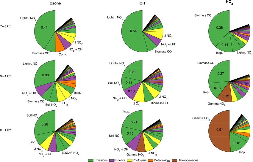
2444                                                              K. E. Christian et al.: INTEX-NA global sensitivity analysis

understood and cannot be perfectly represented in computer          Consortium on Atmospheric Transport and Transformation
models. To make sense of these shortcomings, sensitivity and        (ICARTT). The INTEX-NA (INTEX-North America) part of
uncertainty analyses are useful tools in both determining the       the ICARTT campaign took place in two phases: INTEX-A
robustness of modeled results and identifying and quantify-         (summer 2004) and INTEX-B (spring 2006). The INTEX-
ing sources of error. Generally, sensitivity analyses fall into     A campaign sought to characterize the air chemistry of the
two main camps: local and global. Local sensitivity analyses        eastern and central United States and Canada and was based
involve the perturbation of individual model inputs one at a        out of Pease Air National Guard Base in Portsmouth, New
time over a prescribed segment of the input space. Global           Hampshire and MidAmerica Airport/Scott Air Force Base in
sensitivity analyses, however, feature the simultaneous per-        western Illinois (St. Louis, Missouri metropolitan area). Af-
turbation of multiple inputs across the breadth of their uncer-     ter INTEX-A, which characterized the air composition of the
tainty ranges (Rabitz and Aliş, 1999; Saltelli et al., 2008).      continent, INTEX-B sought to study both the North Pacific
The advantage of these simultaneous perturbations is that           background and Asian outflow, and Mexican outflow over
nonlinear interactions between model factors are allowed to         the Gulf of Mexico. These flights were based out of Hous-
propagate in global sensitivity analysis, an important advan-       ton, Texas; Honolulu, Hawaii; and Anchorage, Alaska.
tage considering the nonlinear nature of the interactions be-          Through a global sensitivity analysis of modeled oxidants
tween emissions, chemistry, and meteorology that underlie           during INTEX, we aim to meet a few goals. The first one is
atmospheric composition modeling.                                   to determine the uncertainty in modeled results arising from
   With the computationally expensive nature of running             uncertainty in the model inputs. The second goal is to de-
chemical transport models (CTMs) such as the GEOS-Chem              termine which of these inputs are most responsible for the
(Goddard Earth Observing System – Chemistry) model used             uncertainty in the modeled results. The third goal is to de-
in this study, global sensitivity methods, which require hun-       termine which perturbations to the model allow for a better
dreds of model runs to provide meaningful statistical results,      match to in situ observations collected during the campaigns.
have been unsurprisingly lacking from the literature, save for      In allowing for the calculation of model uncertainties and
some recent work (Brewer et al., 2017; Christian et al., 2017).     sensitivities to many input factors, a global sensitivity anal-
Instead, the sensitivity analyses of GEOS-Chem modeled re-          ysis is well suited for these objectives. Knowing the model
sults have either used local methods in which the factor of         sensitivities will provide direction not only for future model
interest is perturbed individually and compared to the model        improvements but also for identifying the most impactful di-
state without this perturbation or the GEOS-Chem adjoint            rections for future research.
(Henze et al., 2007). These local and adjoint tests have been
completed for a variety of emissions (e.g., Fiore et al., 2002,
2005; Guerova et al., 2006; Jaeglé et al., 2005; Mao et al.,        2     Methods
2013b; Xu et al., 2013; Qu et al., 2017), meteorological (Wu
et al., 2007; Heald et al., 2010), and chemical factors (Mao        In the following section, we briefly describe the methods em-
et al., 2013a; Newsome and Evans, 2017). While adjoint              ployed in this study. For a more detailed description, please
methods have improved our understanding of atmospheric              refer to Christian et al. (2017).
processes and helped in ascertaining various emissions, there
are some drawbacks when compared to global sensitivity              2.1    Model
methods. For one, without perturbing factors across the en-
tirety of their uncertainty ranges, adjoint sensitivity analy-      We use in this study the default GEOS-Chem model (v9-02),
ses do not provide a complete picture of model uncertainty.         a widely used global chemical transport model (Bey et al.,
Additionally, adjoint sensitivity methods can only provide          2001). There are a few different resolutions available to mod-
model sensitivities for one model output or cost function at        elers, but to facilitate the construction of our sensitivity en-
a time. With global sensitivity analyses, we can calculate          semble, we used the coarser horizontal resolution of 4◦ × 5◦ .
model sensitivities for a variety of different model outputs        Model resolution is an important consideration for chemi-
and domains for negligible additional computational cost.           cal transport models, but the errors associated with resolu-
The drawback for this flexibility in global sensitivity anal-       tion choices are usually less than those coming from chem-
yses is the high computational cost of creating hundreds of         istry, meteorology, and emissions (Wild and Prather, 2006).
chemical transport model runs. Considering the popularity of        In general, there were typically small differences between
adjoint and other sensitivity analysis methods, we see value        modeled results using either 4◦ × 5◦ or 2◦ × 2.5◦ resolutions
in exploring this different and complementary method.               (Figs. S1, S2, S3, and S4 in the Supplement) but we illustrate
   To gain a better grasp of air chemical processes over North      in our results where this is not the case.
America, and the regions both up- and downwind of the con-             Our GEOS-Chem model runs were driven by the Modern-
tinent, various academic and governmental entities took part        Era Retrospective Analysis for Research (MERRA) meteo-
in the NASA-sponsored Intercontinental Chemical Transport           rological model for INTEX-A, while the INTEX-B model
Experiment (INTEX) campaigns, part of the International             runs were driven by GEOS-5 (Goddard Earth Observing Sys-

Atmos. Chem. Phys., 18, 2443–2460, 2018                                              www.atmos-chem-phys.net/18/2443/2018/
K. E. Christian et al.: INTEX-NA global sensitivity analysis                                                                      2445

tem). This difference is due to GEOS-5 model availability          (HOx ≡ OH + HO2 ) reaction (Mao et al., 2013a). Not only
not extending far enough back in time to facilitate its inclu-     is there uncertainty in the rate of this uptake, but there is also
sion in the INTEX-A runs. When comparing modeled results           uncertainty in the product of this reaction, and whether or not
for INTEX-B running MERRA, there were extremely small              H2 O2 is produced instead of or alongside H2 O. In this study,
differences between the modeled results using either mete-         we generally find small differences between these possibili-
orological model. As uncertainties are not published for the       ties.
meteorological models, we define our meteorological uncer-
tainties as the average of the monthly standard deviations of      2.2    Global sensitivity analysis
the difference between GEOS-4 and GEOS-5 meteorologi-
cal fields for 2005, a year of featuring meteorological data       The random sampling – high dimensional model representa-
availability from both models.                                     tion (RS-HDMR) (Rabitz and Aliş, 1999; Li et al., 2001) is
   Generally, the model ensemble made use of the default           a global sensitivity analysis method used in conjunction with
emissions inventories. For many industrialized regions, in-        other air chemistry studies (Chen and Brune, 2012; Chen
cluding much of North America, Europe, and east Asia, the          et al., 2012; Christian et al., 2017). The method involves
regional emissions inventories overwrote the default Emis-         the simultaneous perturbation of model factors across their
sion Database for Global Atmospheric Research (EDGAR)              respective uncertainties. Instead of randomly sampling the
or REanalysis of the TROpospheric chemical composi-                input space as prescribed, we sample using a quasi-random
tion (RETRO) fields. Lightning NOx is treated through the          number sequence (Sobol, 1976). Quasi-random sampling al-
scheme of Price and Rind (1992) with close to a factor of 2        lows for a more efficient sampling of the input space, facil-
greater lightning NOx yield over the midlatitudes compared         itating reliable results with fewer runs. Following common
to the tropics (500 mol flash−1 vs. 260 mol flash−1 ). The dif-    practice, we discarded a set of initial values when creating
ferential between the treatment of tropical and midlatitudinal     the quasi-random sequence, in our case the first 512, as a
NOx yields was created to match observations (Huntrieser           spinup.
et al., 2007, 2008; Hudman et al., 2007). Recent research             Previous sensitivity analyses implementing the HDMR
has questioned the arbitrary geographic boundary in light-         method or its variations often use thousands of model runs.
ning NOx yields and shows the sensitivity of regions around        With CTMs like GEOS-Chem, this computational cost is
the tropical/midlatitude boundary to this treatment (Zhang         prohibitive. Instead, we limit our ensemble to 512 model
et al., 2014; Travis et al., 2016). We show in our results where   runs. As seen in Lu et al. (2013) and this study, we find the
this is a consideration. Transport of stratospheric ozone into     sensitivity results to converge after a few hundred runs, sup-
the troposphere is parameterized by the Synoz algorithm            plying confidence in the indices calculated here.
(McLinden et al., 2000) in which 500 Tg yr−1 of ozone is              Conceptually, the HDMR method describes the modeled
advected through the tropopause.                                   output as a collection of polynomials relating the model out-
   Uncertainties in emissions in this study ranged from fac-       put to the inputs, both individually and collectively.
tors of 2 to 3 with higher uncertainties in biomass and soil                          n
                                                                                      X                  X
emissions. This higher uncertainty is due to the wide range of     f (x) = f0 +             fi (xi ) +           fij (xi , xj )
                                                                                      i=1                1≤i≤n
values in the literature, (e.g., Jaeglé et al., 2005; Schumann
and Huntrieser, 2007; Vinken et al., 2014). While some of                 + . . . + f12...n (x1 , . . ., xn )                       (1)
the uncertainties in these emissions are correlated in reality,
we treat all the emitted species within these emissions in-           Here, f0 is the zeroth-order component, a constant equiv-
ventories individually in this analysis. This treatment allows     alent to the mean (Eq. 2) (where s represents the model run
for the pinpointing of the individual species or processes re-     and N represents the total number of model runs), fi (xi ) is
sulting in model uncertainty. We assume uncertainties of a         the first-order effect corresponding to the independent effect
factor of 2 for lightning NOx (Liaskos et al., 2015), biogenic     of the input xi on the output (Eq. 3) (where i = 1, 2, . . . , n,
VOC (Guenther et al., 2012), stratospheric–tropospheric ex-        where n is the number of factors included in the analysis),
change of ozone, default and regional anthropogenic, ship,         and fij corresponds to the second-order effect on the output
and methyl bromoform emissions.                                    of inputs xi and xj working cooperatively to influence the
   Chemical rate uncertainties came from NASA’s Jet Propul-        output (where i = 1, 2, . . . , n; j = 1, 2, . . . , n; and i 6= j ),
sion Laboratory (JPL) evaluation (Sander et al., 2011). For        down to the nth-order effect on the output by all the inputs
the most part, chemical rate uncertainties are lower than          working cooperatively (Rabitz and Aliş, 1999).
those of emissions inventories, at around 20–30 % for many
                                                                             N
chemical kinetic and photolysis rates. Uncertainty in the rate            1 X
                                                                   f0 ≈         f (x s )                                            (2)
of aerosol particle uptake of the hydroperoxyl radical (HO2 )             N s=1
(gamma HO2 ) was assumed to be a factor of 3. In the case                       ki
of gamma HO2 , we use the default model treatment in which
                                                                                X
                                                                   fi (xi ) ≈         αri ϕr (xi )                                  (3)
γHO2 = 0.2 (Jacob, 2000) and yields H2 O, a terminal HOx                        r=1

www.atmos-chem-phys.net/18/2443/2018/                                                     Atmos. Chem. Phys., 18, 2443–2460, 2018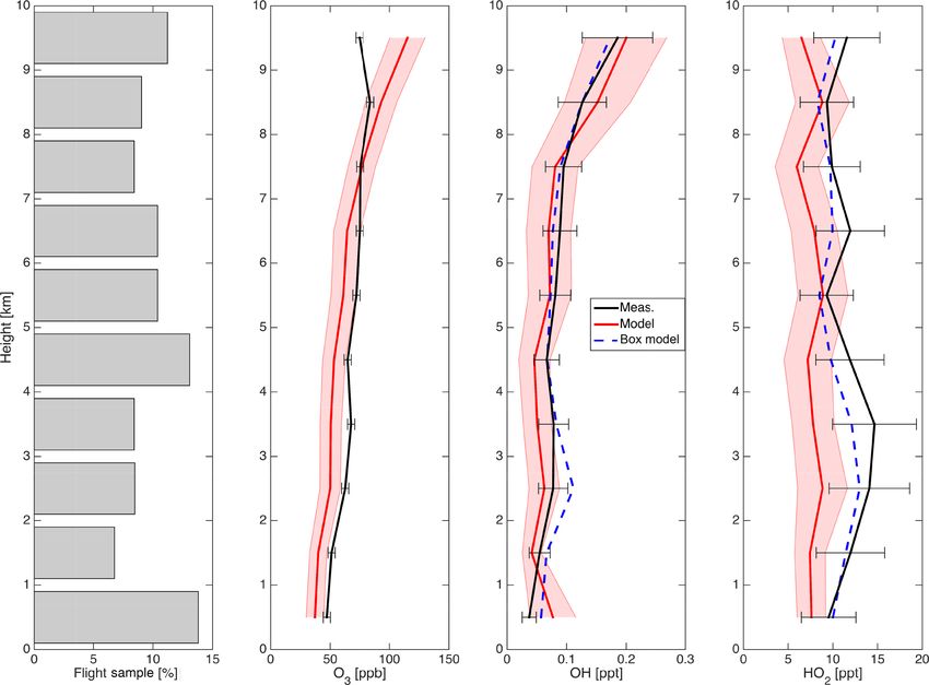
2446                                                                                    K. E. Christian et al.: INTEX-NA global sensitivity analysis

Table 1. Factors included in INTEX-A random sampling – high dimensional model representation (RS-HDMR) analysis and their respec-
tive uncertainties. OC is organic carbon, MP is methyl hydroperoxide, and MO2 is methyl peroxy radical. Uncertainties are expressed as
multiplicative factors, except as noted in meteorological factors.

                        Factor                                                   Uncertaintya              Factor                     Uncertaintya
                        Emissions                                                                          Photolysis
                        Biomass CO, NOx , OC                                                               j [BrNO3 ]                             1.4f
                                                                                            3.0c
                        Soil NOx                                                                           j [CH2 O]                              1.4f
                        Methyl bromoform (CHBr3 )                                                          j [H2 O2 ]                             1.3f
                        EPA (USA) CO, NH3 , NOx                                                            j [HNO3 ]                              1.3f
                                                                                              2.0
                        Street (east Asian) CO, NH3 , NOx , SO2                                            j [HOBr]                               2.0f
                        Ship NOx                                                                           j [NO2 ]                               1.2f
                        Isoprene                                                            2.0d           j [O3 ]                                1.2f
                        Lightning NOx                                                       2.0e           Meteorology
                        Kinetics                                                                           Cloud mass flux                       1.5h
                        k[HNO2 ] [OH]                                                        1.5f          Relative humidity                    5 %i
                        k[HNO3 ] [OH]                                                        1.2f          Soil wetness                       8.8 %g
                        k[HO2 ] [HO2 ]                                                1.15/1.2b,f          Specific humidity                    5 %i
                        k[HO2 ] [NO]                                                       1.15f           Temperature                        1.8 Kg
                        k[MO2 ] [HO2 ]                                                       1.3f          Heterogeneous
                        k[MO2 ] [NO]                                                       1.15f           Gamma HO2                              3.0f
                        k[NO2 ] [OH]                                                         1.3f
                        k[O3 ] [HO2 ]                                                      1.15f
                        k[O3 ] [NO]                                                         1.1f
                        k[OH] [CH4 ]                                                        1.1f
                        k[OH] [HO2 ]                                                       1.15f
                      a At 1σ uncertainty confidence. b High-pressure limit/low-pressure limit uncertainties. c Jaeglé et al. (2005). d Guenther et
                      al. (2012). e Liaskos et al. (2015). f Sander et al. (2011). g GEOS-5 – GEOS-4. h Ott et al. (2009). i Heald et al. (2010).

                                                                                           creation of sensitivity indices for each input (Eq. 5). While
   Here, ϕ represents orthonormal polynomials, ki represents                               sensitivity indices can similarly be found for the functions
the orders of the polynomials fitted for each input, and α                                 relating to the second- and higher-order interactions between
is the constant coefficient for each polynomial. Similarly to                              inputs, these indices need more model runs than presented
Eq. (3), polynomials created to represent second- and higher-                              here for meaningful results. The end result of the sensitiv-
order effects such as fij (xi , xxj ) are created using orthonor-                          ity index calculations is a series of sensitivity indices repre-
mal polynomials and constant coefficients. For a more de-                                  senting the portion of the output variance attributable to each
tailed description of the calculation of the orthonormal basis                             input factor with the residual portion attributable to second-
polynomials (ϕ) and the constant coefficients (α), refer to Li                             and higher-order factor–factor interactions (Eq. 6).
et al. (2002, 2003).                                                                          V (fi (xi ))
   With each component function being orthogonal, the total                                Si =                                                          (5)
variance can be split into a summation of the variances of all                                V (f (x)))
                                                                                              n
the polynomials in Eq. (3) (e.g., Li et al., 2010). For example,                              X
                                                                                           1=    Si + higher-order sensitivities                         (6)
              n                                                                                   i=1
              X                        X
V (f (x)) =         V (fi (xi )) +           V (fij (xi , xj ))                            To focus the RS-HDMR analysis on the most important
              i=1                    1≤i≤n                                                 model inputs, we completed a preliminary Morris method
          + . . . + V (f12...n (x1 , . . ., xn )),                              (4)        sensitivity test (Morris, 1991) for both the INTEX-A and
                                                                                           INTEX-B domains, including any factor within around 15 %
where V (fi (xi )) represents the variance of the first-order ef-                          of the most sensitive factor for ozone, OH, or HO2 . Using the
fect due to the input xi and so forth. Normalizing the indi-                               Morris method as a preliminary step in RS-HDMR tests is a
vidual variances in Eq. (4) by the total variance results in the                           common practice in multiple RS-HDMR sensitivity studies

Atmos. Chem. Phys., 18, 2443–2460, 2018                                                                              www.atmos-chem-phys.net/18/2443/2018/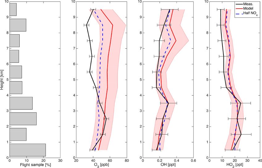
K. E. Christian et al.: INTEX-NA global sensitivity analysis                                                                                             2447

Table 2. Factors included in INTEX-B RS-HDMR analysis and their respective uncertainties. OC is organic carbon, MP is methyl hydroper-
oxide, and MO2 is methyl peroxy radical. Uncertainties are expressed as multiplicative factors, except as noted in meteorological factors.

                    Factor                                                   Uncertaintya              Factor                       Uncertaintya
                    Emissions                                                                          Photolysis
                    Biomass CO, NH3 , NOx , OC                                                         j [CH2 O]                                  1.4f
                                                                                        3.0c
                    Soil NOx                                                                           j [H2 O2 ]                                 1.3f
                    Methyl bromoform (CHBr3 )                                                          j [HNO3 ]                                  1.3f
                    EDGAR NOx                                                                          j [HOBr]                                   2.0f
                    EMEP (European) NOx                                                                j [MP]                                     1.5f
                    EPA (USA) CO, NOx                                                     2.0          j [NO2 ]                                   1.2f
                    Street (east Asian) CO, NH3 , NOx , SO2                                            j [O3 ]                                    1.2f
                    Ship NOx                                                                           Meteorology
                    Strat–trop exchange O3                                                             Cloud fraction                      8.5 %g
                    Isoprene                                                            2.0d           Cloud mass flux                            1.5h
                    Lightning NOx                                                       2.0e           Relative humidity                          5 %i
                    Kinetics                                                                           Soil wetness                        8.8 %g
                    k[HNO3 ] [OH]                                                      1.2f            Specific humidity                    5 %i
                    k[HO2 ] [HO2 ]                                              1.15/1.2b,f            Temperature                        1.8 Kg
                    k[HO2 ] [NO]                                                     1.15f             U wind                        0.71 ms−1g
                    k[MO2 ] [HO2 ]                                                       1.3f          Heterogeneous
                    k[MO2 ] [NO]                                                       1.15f           Gamma HO2                               3.0f
                    k[MP] [OH]                                                           1.4f          Gamma NO2                               3.0f
                    k[NO2 ] [OH]                                                        1.3f           Henry’s law HOBr                       10.0f
                    k[O3 ] [HO2 ]                                                      1.15f
                    k[O3 ] [NO]                                                         1.1f
                    k[O3 ] [NO2 ]                                                      1.15f
                    k[OH] [CH4 ]                                                        1.1f
                    k[OH] [HO2 ]                                                       1.15f
                  a At 1σ uncertainty confidence. b High-pressure limit/low-pressure limit uncertainties. c Jaeglé et al. (2005). d Guenther et
                  al. (2012). e Liaskos et al. (2015). f Sander et al. (2011). g GEOS-5 – GEOS-4. h Ott et al. (2009). i Heald et al. (2010).

(Ziehn et al., 2009; Chen et al., 2012; Lu et al., 2013). This                          the model ensemble were spun up 9 months before the first
prescreening process resulted in 39 factors being included in                           flight for the respective campaigns.
the RS-HDMR analysis for INTEX-A and 47 for INTEX-B
(Tables 1 and 2, respectively).                                                         2.2.2      Calculation of sensitivity indices

                                                                                        RS-HDMR sensitivity indices were calculated using graph-
2.2.1   Uncertainties
                                                                                        ical user interface – HDMR (GUI-HDMR), a free MAT-
                                                                                        LAB package (http://www.gui-hdmr.de) (Ziehn and Tomlin,
Before perturbing the inputs and running the model, the                                 2009). As in Christian et al. (2017), in running GUI-HDMR,
next step was to create the uncertainty distributions for the                           the inputs were scaled according to their percentiles within
prescreened model inputs using the uncertainties listed ear-                            their respective uncertainty distributions and the correlation
lier in the methods section and in Tables 1 and 2. For the                              method option was applied (Kalos and Whitlock, 1986; Li
majority of the factors, we used lognormal uncertainty dis-                             et al., 2003).
tributions where the standard deviations were determined
by σ = (f − 1/f )/2 (Gao et al., 1995; Yang et al., 1995)                               2.3     Measurements
where f is the published uncertainty factor. Normal distri-
butions were used for some meteorological factors (relative                             The NASA DC-8 carried a suite of state-of-the-science in-
and specific humidity, soil wetness, and temperature). To al-                           struments during both INTEX-A and INTEX-B (Singh et al.,
low model perturbations’ time to spread globally, all runs in                           2006, 2009). For comparison to the modeled HOx mixing

www.atmos-chem-phys.net/18/2443/2018/                                                                           Atmos. Chem. Phys., 18, 2443–2460, 2018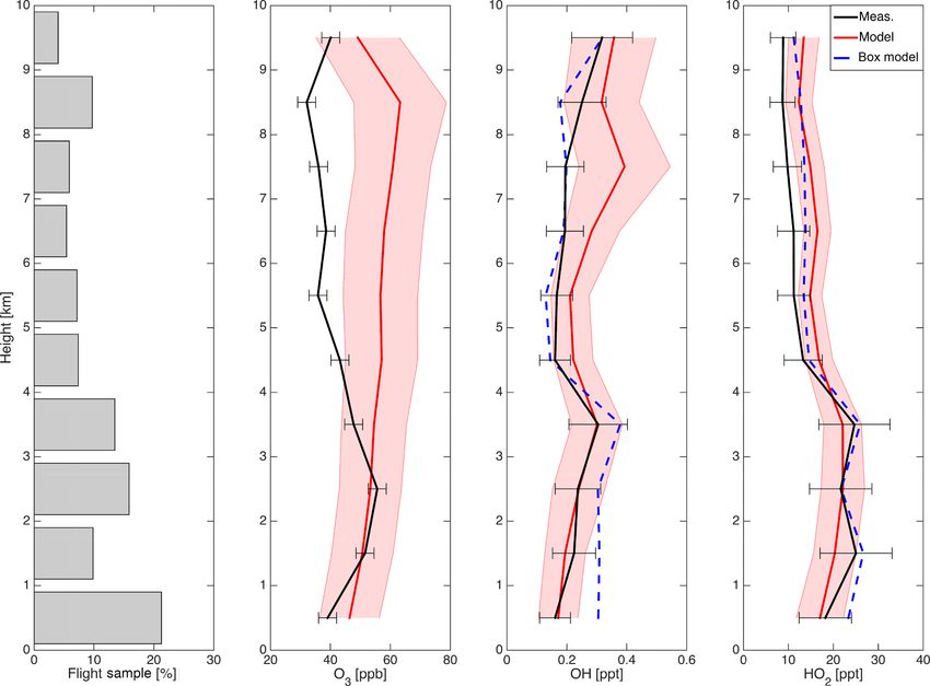
2448                                                              K. E. Christian et al.: INTEX-NA global sensitivity analysis

ratios, we compare to the measurements taken by Pennsylva-
nia State University’s Airborne Tropospheric Hydrogen Ox-
ides Sensor (ATHOS) (Brune et al., 1998). In this instrument,
HOx is measured using laser-induced fluorescence (LIF).
Ozone mixing ratios were measured by NASA-LaRC (Lan-
gley Research Center) using nitric oxide chemiluminescence
(Weinheimer et al., 1994).
   Interferences in OH and HO2 measurements are a concern
with ATHOS and other measurement techniques (Ren et al.,
2004; Fuchs et al., 2011; Mao et al., 2012). Typically these        Figure 1. Map of INTEX-A & INTEX-B flights.
interferences are less than a factor of 2 for HO2 and between
a factor of 1.2 and 3 for OH. Interferences in OH and HO2
are mostly a concern in the boundary layer above forested or        Mexico and the North Pacific (Fig. 1) in the spring of 2006.
urban environments as they occur in the presence of alkenes         In both campaigns, the aircraft sampled the troposphere at a
or aromatics. For much of the middle to upper troposphere           variety of altitudes from the surface to near the tropopause
and the marine domains sampled in much of INTEX-B, these            (bar graphs in Figs. 2, 3, 4, and 5). In INTEX-B, the results
interferences will be negligible.                                   are split into three separate domains outlined in Fig. 1 and
                                                                    named according to the city in which the flights were based:
2.4    Box model
                                                                    Houston, Texas; Honolulu, Hawaii; and Anchorage, Alaska.
In contrast to our previous study, we also analyze oxi-
                                                                    3.1     Uncertainty
dant mixing ratios calculated by a time-dependent zero-
dimensional box model providing an additional comparison            3.1.1    INTEX-A
to both the chemical transport model and the measurements.
In this modeling approach, HOx mixing ratios are calculated         For ozone and OH, GEOS-Chem modeled mixing ra-
using a model constrained by other trace gas measurements           tios were consistently higher than measurements (Fig. 2).
measured aboard the DC-8 and are integrated until the box           Throughout the vertical column, GEOS-Chem modeled
model reaches a consistent diurnal steady state. At a min-          ozone was around 10 ppb greater than measurements. For
imum, the model is constrained by ozone, CO, NO2 , non-             OH, modeled and measured values were similar close to the
methane hydrocarbons, acetone, methanol, temperature, dew           surface, but the disagreement widened higher, with modeled
and frost point of water, pressure, and calculated photolysis       values being a factor of ∼ 1.6 greater than measurements
frequencies (Ren et al., 2008). These model calculations are        around 6 km. Unlike GEOS-Chem, the box model generally
available alongside the measurements in the NASA Langley            agreed with the measured OH profiles, suggesting that the
archives for the campaigns. For a more detailed description         model errors for OH are likely arising outside of the chemical
of the box model, please refer to Crawford et al. (1999), Ol-       mechanism, such as emissions sources. In contrast to ozone
son et al. (2004), and Ren et al. (2008).                           and OH, measured HO2 profiles were generally greater than
                                                                    the model ensemble, with the widest disagreement coming
2.5    Comparison of modeled and measured results
                                                                    close to the surface. Unlike OH, HO2 profiles modeled by
Allowing for the comparison of the model ensemble to the            the box model generally agreed with GEOS-Chem more than
aircraft observations, modeled results were output in 1 min         they did with the measurements. This model–model agree-
intervals along the DC-8 flight track using the Planeflight op-     ment suggests that either the model errors may be arising
tion within GEOS-Chem. With a relatively coarse horizontal          from the largely similar chemistry of the two models or
resolution chosen, it is a concern that GEOS-Chem would             the measurements are incorrect, perhaps due to peroxy rad-
miss meso- to synoptic-scale features that could be important       ical interference. The agreement between GEOS-Chem and
for correctly modeling oxidant abundances. With our analy-          ATHOS HOx profiles presented here is different than in Hud-
sis averaging over many flights, many of these differences          man et al. (2007) due to errors found in the calibration of the
would be averaged out.                                              measurements (Ren et al., 2008). At all altitudes, there were
                                                                    small differences between the finer 2◦ × 2.5◦ and the coarser
                                                                    4◦ × 5◦ ensemble. Specifically, these differences were less
3     Results                                                       than 4 ppb for ozone, a few hundredths of a ppt for OH, and
                                                                    less than 1 ppt for HO2 .
During INTEX-A, the NASA DC-8 primarily sampled the                    Part of this disagreement in mixing ratios could be at-
eastern half of the United States and Canada during the sum-        tributed to uncertainties in the modeled values. We find 1σ
mer of 2004. In contrast to the mostly continental study area       uncertainties for the modeled oxidant mixing ratios to range
of INTEX-A, INTEX-B largely took place over the Gulf of             from 19 to 23 % for ozone, 27 to 36 % for OH, and 18 to

Atmos. Chem. Phys., 18, 2443–2460, 2018                                              www.atmos-chem-phys.net/18/2443/2018/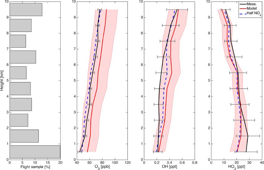
K. E. Christian et al.: INTEX-NA global sensitivity analysis                                                                    2449

Figure 2. Vertical profiles of median modeled (red) and measured     Figure 3. Vertical profiles of median modeled (red) and measured
(black) ozone, OH, and HO2 for INTEX-A flight data binned by         (black) ozone, OH, and HO2 for Houston-based INTEX-B flight
kilometer. Gray bar graph shows percent of flight data within each   data binned by kilometer. Gray bar graph shows percent of flight
vertical bin. Shaded regions represent 1σ of the model ensemble;     data within each vertical bin. Shaded regions represent 1σ of the
error bars on measurements are uncertainty at 1σ confidence. Blue    model ensemble; error bars on measurements are uncertainty at 1σ
line represents results from the box model (Ren et al., 2008).       confidence. Blue line represents results from the box model.

37 % for HO2 in the different vertical bins. When taking into           Unlike GEOS-Chem, the box model tended to better agree
account both uncertainties in model input factors and mea-           with measurements higher in the troposphere for OH (Fig. 3).
surements, we find there to be overlap between all the oxi-          In the case of OH mixing ratios, the box model was around
dant profiles. This overlap shows that the uncertainties in the      a factor of 2 greater than measurements in the first vertical
model and measurements can explain the difference between            bin and around 30 % greater up to 4 km. Higher than 4 km,
the model and measured profiles.                                     the box model and measurements largely agreed. For HO2
                                                                     mixing ratios, the box model was greater than observations
3.1.2   INTEX-B Houston                                              at all heights but was marginally closer than GEOS-Chem to
                                                                     the measured profile.
The vertical profiles for ozone, OH, and HO2 all follow a
                                                                        Model ozone uncertainty was largely altitude independent,
similar pattern: general agreement between measured and
                                                                     running between 19 and 21 % below 8 km. Uncertainty in
modeled mixing ratios near the surface turning to model
                                                                     modeled OH was between 28 and 40 %, with uncertainty on
overestimation above 4 km or so (Fig. 3). In the case of
                                                                     a percentage basis ranging highest near the surface and above
ozone, the model–measurement gap persists even when ac-
                                                                     7 km (Fig. 3). Model HO2 uncertainty followed a similar ver-
counting for measurement uncertainty, especially from 5 km
                                                                     tical pattern to OH with the highest uncertainty coming near
higher. As a consequence of this model overprediction of
                                                                     the surface (∼ 30 %) and lower in the middle troposphere
ozone, OH and HO2 both are also overpredicted by GEOS-
                                                                     (18–20 % from 3 km up to 8 km).
Chem above 4–5 km, but unlike ozone, there is overlap at all
levels between the measured and modeled values when un-
                                                                     3.1.3   INTEX-B Honolulu
certainties in both are taken into account. Generally, there are
small differences between the median of the 4◦ × 5◦ model
                                                                     Vertically, uncertainty in ozone is nearly altitude indepen-
ensemble and a finer resolution 2◦ × 2.5◦ run; however, there
                                                                     dent, ranging between 17.5 and 20.5 % (1σ ) (Fig. 4). While
are some larger differences between these two possibilities,
                                                                     GEOS-Chem on average comes close to the average mea-
with ozone mixing ratios being reduced by 7–9 ppb above
                                                                     sured values, the model fails in matching the measured pro-
5 km in the finer resolution. Conversely, below 5 km, the
                                                                     file shape. Near the surface, GEOS-Chem is around 12 ppb
finer resolution run produces higher OH mixing ratios (about
                                                                     less than measured values. This underprediction shifts to
0.06 ppt or ∼ 30 % higher), roughly on the order of the 1σ
                                                                     overprediction around 4 km, with the model overpredict-
model uncertainty. Differences between HO2 profiles using
                                                                     ing 25–30 ppb around 9–10 km. This under- and overpredic-
either model resolution were within a few ppt at all altitudes
                                                                     tion by the model at low and high altitudes is outside the
and within 1 ppt in most of the vertical bins.
                                                                     model and measurement uncertainties. Differences between
                                                                     the finer 2◦ × 2.5◦ and the coarser 4◦ × 5◦ ensemble were
                                                                     smaller than these model–measurement disagreements. At

www.atmos-chem-phys.net/18/2443/2018/                                                 Atmos. Chem. Phys., 18, 2443–2460, 2018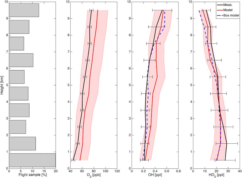
2450                                                                K. E. Christian et al.: INTEX-NA global sensitivity analysis

                                                                      the model around 10 ppb, with the difference between mod-
                                                                      eled and measured values maxing out at 17 ppb around 4 km.
                                                                      Except for near the surface where the model was around
                                                                      0.04 ppt too high and above 8 km, GEOS-Chem generally un-
                                                                      derrepresented OH by a couple hundredths of a ppt. These
                                                                      differences are within the model and measurement uncer-
                                                                      tainty. HO2 mixing ratios showed some of the widest dis-
                                                                      agreement between modeled and measured values, with the
                                                                      model being anywhere from 1.6 ppt short near the surface to
                                                                      upwards of 6.8 ppt between 3 and 4 km. In this domain, we
                                                                      found small differences in oxidant mixing ratios between the
                                                                      finer 2◦ ×2.5◦ and the coarser 4◦ ×5◦ ensemble. Specifically,
                                                                      modeled ozone was around 0–4 ppb higher in the fine reso-
                                                                      lution case, OH 1–3 hundredths of a ppt higher in the fine
                                                                      resolution case, and HO2 mixing ratios within a few tenths
                                                                      of a ppt.
Figure 4. Vertical profiles of median modeled (red) and measured
(black) ozone, OH, and HO2 for Honolulu-based INTEX-B flight
                                                                         Compared to GEOS-Chem, the box model performs better
data binned by kilometer. Gray bar graph shows percent of flight      in matching the measured OH and HO2 mixing ratio profiles.
data within each vertical bin. Shaded regions represent 1σ of the     In particular, while still somewhat underpredicting HO2 mix-
model ensemble; error bars on measurements are uncertainty at 1σ      ing ratios, the box model does match the shape of the mea-
confidence. Blue line represents results from the box model.          sured HO2 profile unlike GEOS-Chem (Fig. 5). Because of
                                                                      this relatively close match between the box model and the
                                                                      measurements, the disagreement between GEOS-Chem and
nearly every altitude, the ozone mixing ratios were within            the measurements could be arising outside of the chemical
10 ppb with no consistent positive or negative bias.                  kinetics. Conversely, the box model may be better matching
   In contrast to ozone, the uncertainty in OH mixing ratios is       the measured profile just due to its lack of aerosol uptake
high and vertically variable (Fig. 4). From 0 to 3 km, uncer-         of HO2 . In the Arctic, the aerosol uptake of HO2 is a major
tainty is roughly around 32–36 % before increasing through            loss pathway for HO2 (Whalley et al., 2015). Without this
the middle troposphere to 38–40 %. For all altitudes, mea-            loss pathway, the box model may have artificially high HO2
sured and model values were within each other’s uncertainty           mixing ratios.
range. The box model agreed well with OH measured mixing                 Uncertainty in modeled ozone mixing ratios was relatively
ratios, especially above 5 km with more modest agreement              low, ranging between 13 and 20 %. In contrast, uncertainties
and slight overprediction below. Between the finer 2◦ × 2.5◦          in both OH and HO2 mixing ratios were considerable, rang-
and the coarser 4◦ × 5◦ ensemble we found generally higher            ing between 34 and 57 % for OH and 21 and 40 % for HO2
OH mixing ratios but within a few hundredths of a ppt.                (Fig. 5). This higher uncertainty is in part a product of the
   Compared to OH, uncertainty in HO2 mixing ratios is                very low mixing ratios modeled in this northern domain with
lower but follows the same pattern of increasing with alti-           OH mixing ratios being less than a tenth of a ppt for most
tude (Fig. 4). We find uncertainty rising from 16–20 % be-            of the vertical column and modeled HO2 mixing ratios in a
tween the surface and 4 km to between 23 and 30 % from                range between 6 and 9 ppt.
5 km higher. Generally, GEOS-Chem replicated the mea-
sured HO2 mixing ratio profile within a couple ppt. Differ-           3.1.5   Takeaways from uncertainties
ences between the finer and coarser resolution choices re-
                                                                      Despite the geographic range of the regions presented here,
sulted in differences around or less than 2 ppt below 9 km.
                                                                      there are many similarities to highlight. For instance, uncer-
Like OH, the box model generally agreed well with mea-
                                                                      tainties in GEOS-Chem modeled mixing ratios for ozone,
sured HO2 mixing ratios. The overall agreement between the
                                                                      OH, and HO2 were largely similar. As a rule of thumb, un-
oxidant profiles in this domain may be attributable to the re-
                                                                      certainties in ozone mixing ratios were around 20 %, OH be-
duced surface emissions sources in this remote central Pacific
                                                                      tween 25 and 40 %, and HO2 between 20 and 35 %. Also, for
domain.
                                                                      most regions, when uncertainties in both GEOS-Chem and
3.1.4   INTEX-B Anchorage                                             measurements are taken into account, there is general agree-
                                                                      ment between oxidant mixing ratios with the exception of
In contrast to the previous regions analyzed here, measured           ozone profiles in the higher-altitude Houston-based INTEX-
ozone, OH, and HO2 mixing ratios were generally greater               B flights and ozone in a few other vertical bins in the Pacific
than GEOS-Chem modeled values in nearly every vertical                INTEX-B flights.
bin (Fig. 5). Ozone mixing ratios were underpredicted by

Atmos. Chem. Phys., 18, 2443–2460, 2018                                                www.atmos-chem-phys.net/18/2443/2018/
K. E. Christian et al.: INTEX-NA global sensitivity analysis 2451
Near the surface where modeled aerosol concentrations
are greatest, HO2 is most sensitive to the aerosol uptake of
HO2 and isoprene emissions (Si = 0.28 and 0.25, respec-
tively) (Fig. 2). This sensitivity to aerosol uptake is reduced
higher in the troposphere with biomass CO (Si = 0.26 at
3–4 km and Si = 0.18 between 7 and 8 km), lightning NOx
(Si = 0.12 at 7–8 km), and isoprene emissions (Si = 0.15 be-
tween 3 and 4 km and Si = 0.26 between 7 and 8 km) being
the dominant sources of the uncertainty above 3 km. As un-
certainty in gamma HO2 is not limited to just the rate of the
reaction but also to the product, we examined the modeled
profiles in a model run having gamma HO2 producing H2 O2
rather than H2 O. With small differences generally around or
less than half a ppt for HO2 and likewise small differences
for OH and ozone, HO2 and the other oxidants are rather
insensitive to this difference. Sensitivity to isoprene emis-
Figure 5. Vertical profiles of median modeled (red) and measured
(black) ozone, OH, and HO2 for Anchorage-based INTEX-B flight
sions is roughly altitude independent. As isoprene’s lifetime
data binned by kilometer. Gray bar graph shows percent of flight is shorter than the timescales to allow consequential trans-
data within each vertical bin. Shaded regions represent 1σ of the port past the boundary layer, the sensitivity of HO2 to iso-
model ensemble; error bars on measurements are uncertainty at 1σ prene emissions in the middle to free troposphere is almost
confidence. Blue line represents results from the box model. certainly due to chemistry relating to secondary and higher-
order isoprene products such as the photolysis of formalde-
hyde and acetaldehyde.
3.2 Sensitivities
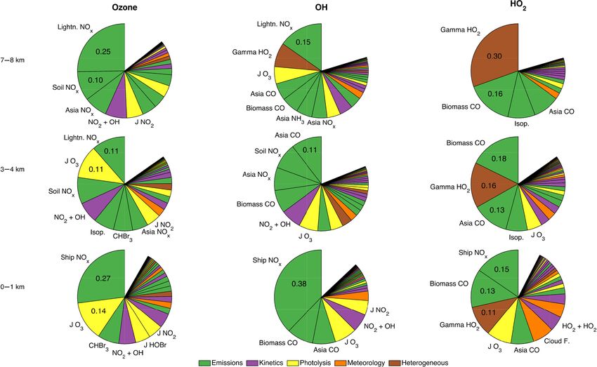
3.2.2 INTEX-B Houston
To explore from where the model–measurement disagree-
ments may be coming, Figs. 6, 7, 8, and 9 show the median As with INTEX-A, ozone is largely sensitive to NOx emis-
first-order sensitivity indices across INTEX-A and regional sion inventories, specifically soil NOx near the surface and
INTEX-B flights for ozone, OH, and HO2 . As the sensitivi- lightning NOx from 3 km higher (Fig. 7). In contrast to the
ties of ozone, OH, and HO2 varied with altitude, we show the height dependencies in the emissions inventories’ sensitiv-
analysis for the 0–1 km, 3–4 km, and 7–8 km vertical bins. ities, sensitivity to chemical factors was generally altitude
The “missing” portion of the pies represents the portion of independent with sensitivities to k[NO2 + OH] ranging be-
the model variance not explained by uncertainties in individ- tween Si values of 0.07 and 0.09, and j [NO2 ] and j [O3 ]
ual factors (rather factor–factor interactions). between 0.03 and 0.08. For emission factors, in the low-
est 1 km, apart from soil NOx emissions (Si = 0.28), we
3.2.1 INTEX-A
also find isoprene emissions (Si = 0.08) and EDGAR NOx
Generally, ozone was most sensitive to emissions, particu- emissions (Si = 0.07) having Si values greater than 0.05.
larly NOx and isoprene (Fig. 6). Near the surface, ozone was From 3 to 4 km higher, lightning NOx becomes the dominant
most sensitive to the EPA-NEI (Environmental Protection source of uncertainty, with Si values of 0.30 around 4 km
Agency – National Emissions Inventory) NOx emissions and and higher between 7 and 8 km (Si = 0.41). In these higher-
isoprene (Si = 0.21 and 0.20, respectively). A few kilome- altitude bins, we also find ozone to have greater sensitivity to
ters up, this sensitivity to surface NOx emissions is replaced biomass CO emissions with Si values of 0.07 between 3 and
by sensitivity to lightning NOx (Si = 0.28 and 0.30 for 3– 4 km, and Si = 0.09 between 7 and 8 km.
4 km and 7–8 km, respectively). Sensitivity to chemical fac- Similar to ozone, while we find OH to be most sensitive
tors such as the NO2 + OH reaction rate and the NO2 photol- to emissions sources, the sensitivity to these sources is alti-
ysis rate were largely altitude independent (Si between 0.08 tude dependent (Fig. 7). Near the surface, OH is most sen-
and 0.13 for k[NO2 + OH]; Si = 0.07 − 0.08 for j [NO2 ]). sitive to isoprene and soil NOx emissions sources (Si val-
Sensitivities for OH largely mirrored those of ozone ues of 0.21 and 0.15, respectively). Chemical factors such
(Fig. 6). As photolysis of ozone in the presence of water va- as k[NO2 + OH], aerosol uptake of HO2 , and j [NO2 ] also
por leads directly to the production of OH, this is unsurpris- had Si values greater than 0.05 (0.09, 0.08, and 0.07, respec-
ing. In addition to NOx and isoprene emissions mentioned tively). Higher, lightning NOx becomes the dominant source
with ozone, we also find OH above 3 km to be sensitive to of uncertainty for OH mixing ratios with Si values of 0.21 in
CO emissions, especially from biomass burning (Si = 0.16 the 3–4 km bin and 0.54 for the 7–8 km bin.
between 3 and 4 km and Si = 0.10 between 7 and 8 km). For HO2 mixing ratios, near the surface, we find gamma
HO2 to be responsible for about half of the model uncertainty
www.atmos-chem-phys.net/18/2443/2018/ Atmos. Chem. Phys., 18, 2443–2460, 20182452 K. E. Christian et al.: INTEX-NA global sensitivity analysis
Figure 6. First-order sensitivity indices for median flight track ozone, OH, and HO2 for INTEX-A flights. Legend categories are defined in
Table 1. Sensitivity indices are labeled in pie slices for factors for which Si ≥ 0.10.
(Si = 0.51), with isoprene emissions being the only other indices ranging between 0.10 and 0.15 between the surface
factor with Si >0.05 (Si = 0.16) (Fig. 7). This dominance and 5 km. The NO2 + OH reaction rate also had sensitivity
by gamma HO2 , though, is restricted to near the surface indices at about 0.07 at most altitudes.
where aerosol concentrations are highest. In fact, higher than OH mixing ratios were largely sensitive to the same factors
3 km, we find biomass CO emissions to become the domi- as ozone (Fig. 8). Near the surface, OH was largely sensitive
nant source of uncertainty (Si = 0.27 for 3–4 km, Si = 0.38 to ship NOx emissions (Si = 0.38), both biomass and east
for 7–8 km). Sensitivity to isoprene emissions is similar be- Asian CO, j [O3 ], k[NO2 + OH], and j [NO2 ] (Si = 0.09,
tween 3–4 and 7–8 km with Si values of 0.13 and 0.14, re- 0.08, 0.08, 0.06, and 0.05, respectively). Above 3 km, there
spectively. is no single factor that overwhelmingly contributes to the un-
certainty, but CO and NOx emissions, along with the photol-
3.2.3 INTEX-B Honolulu ysis rate of ozone and the NO2 + OH reaction rate, all had Si
values greater than 0.05 for the higher-altitude bins.
Like the Houston flights, HO2 mixing ratios were largely
For the flights based out of Honolulu, near-surface ozone was
sensitive to CO emissions, NOx emissions, and aerosol up-
most sensitive to surface emissions sources in the first verti-
take of HO2 ; only sensitivity to aerosol uptake is reversed
cal kilometer with ship NOx (Si = 0.27) and methyl bromo-
vertically with higher sensitivities coming in the upper tro-
form emissions (Si = 0.07) and a variety of chemical fac-
posphere rather than near the surface (Si = 0.10, 0.16, and
tors such as the ozone photolysis rate (j [O3 ] (Si = 0.14),
0.30 for 0–1, 3–4, and 7–8 km vertical bins) (Fig. 8). This is
k[NO2 + OH] (Si = 0.06), j [HOBr] (Si = 0.05), j [NO2 ]
a result of the modeled aerosol concentrations being highest
(Si = 0.05)) (Fig. 8). Higher, ozone becomes sensitive to
near the surface for the Houston flights and highest in the
other emissions sources, especially lightning NOx (Si = 0.11
upper reaches of the troposphere for the Honolulu flights.
and 0.25 at 3–4 km and 7–8 km, respectively), and to a lesser
extent, soil, and east Asian NOx and isoprene emissions.
These latter emissions sources are noteworthy as they illus- 3.2.4 INTEX-B Anchorage
trate the sensitivity of this region to nonlocal upwind emis-
sion sources, as there are not any appreciable isoprene or soil Near the surface, ozone sensitivity was dominated by ship
NOx emissions over the remote north-central Pacific. In addi- NOx emissions (Si = 0.52) and to a much lesser extent pho-
tion to emissions sources, ozone also showed moderate sensi- tolysis of HOBr (Si = 0.06). Higher, a host of emissions
tivity to chemical factors. In particular, the photolysis rate of factors become more important, with bromoform emissions
ozone, in spite of its low uncertainty (20 %), had sensitivity (Si = 0.11 for 3–4 km and Si = 0.09 for 7–8 km), soil NOx
Atmos. Chem. Phys., 18, 2443–2460, 2018 www.atmos-chem-phys.net/18/2443/2018/K. E. Christian et al.: INTEX-NA global sensitivity analysis 2453 Figure 7. First-order sensitivity indices for median flight track ozone, OH, and HO2 for INTEX-B flights originating from and terminating in Houston. Legend categories are defined in Table 2. Sensitivity indices are labeled in pie slices for factors for which Si ≥ 0.10. Figure 8. First-order sensitivity indices for median flight track ozone, OH, and HO2 for INTEX-B flights originating from and terminating in Honolulu. Legend categories are defined in Table 2. Sensitivity indices are labeled in pie slices for factors for which Si ≥ 0.10. www.atmos-chem-phys.net/18/2443/2018/ Atmos. Chem. Phys., 18, 2443–2460, 2018
2454 K. E. Christian et al.: INTEX-NA global sensitivity analysis
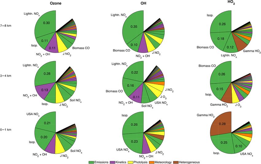
Figure 9. First-order sensitivity indices for median flight track ozone, OH, and HO2 for INTEX-B flights originating from and terminating
in Anchorage. Legend categories are defined in Table 2. Sensitivity indices are labeled in pie slices for factors for which Si ≥ 0.10.
(Si = 0.10 and 0.11 for 3–4 and 7–8 km, respectively), and the inputs, it raises the question: which ensemble members
lightning NOx (Si = 0.13 at 7–8 km) (Fig. 9). Chemical fac- fit the measured profiles best? With 512 model runs with var-
tors such as k[NO2 + OH] and j [NO2 ] also were responsible ious perturbations of the inputs, some members did come
for between 6 and 8 % of the uncertainty for both the 3–4 km much closer to matching the measured profiles. In the fol-
and 7–8 km altitude bins. lowing subsections, we describe the commonalities among
Like ozone, OH was overwhelmingly sensitive to ship these better-performing ensemble members’ perturbations to
NOx emissions (Si = 0.50), with this one factor being re- NOx emissions and aerosol uptake.
sponsible for around half the model uncertainty (Fig. 9). At
3–4 km, this sensitivity to ship NOx emissions is replaced by 3.3.1 NOx emissions
CO emissions from east Asia and biomass burning and soil
NOx (Si = 0.11 for east Asian CO, Si = 0.09 for biomass For all the regions presented here, GEOS-Chem modeled
CO and soil NOx ). From 3 km higher, OH mixing ratios are and measured ozone and OH profiles have closer agreement
most sensitive to the aerosol uptake of HO2 (Si = 0.14 at 3– with lower lightning NOx emissions than those emitted by
4 km, Si = 0.29 at 7–8 km). default. In examining the closest 25 model ensemble mem-
At all but the highest altitudes, modeled HO2 mixing ra- bers for each region and oxidant, we find reductions in their
tios were overwhelmingly sensitive to the aerosol uptake of lightning NOx emissions anywhere from ∼ 25 % for Anchor-
HO2 (gamma HO2 ) with this one factor contributing around age INTEX-B ozone and OH, INTEX-A ozone, and Hon-
half the model uncertainty (Si = 0.49 at 0–1 km, Si = 0.57 olulu INTEX-B OH, to around a factor of 2 reduction for
at both 3–4 and 7–8 km) (Fig. 9). This dominance of gamma INTEX-A OH, Houston INTEX-B ozone and OH, and Hon-
HO2 on HO2 mixing ratios has been noted before in the sim- olulu INTEX-B ozone. Considering GEOS-Chem tended to
ilar ARCTAS-A (Arctic Research of the Composition of the overpredict ozone and OH, especially at higher altitudes, it
Troposphere from Aircraft and Satellites) domain (Christian is unsurprising there is better agreement with lower lightning
et al., 2017). NOx emissions.
The vertical profiles of NO and NO2 (Fig. S5) somewhat
3.3 Discussion of results corroborate this overestimation of NOx emissions in INTEX-
A and can explain the overestimate of ozone. In INTEX-A,
Broadly speaking, measured and GEOS-Chem modeled ox- we found modeled NO2 to be consistently greater than their
idant profiles agreed to some extent in most of the cases respective measured values. Near the surface, this difference
outlined here. However, with 512 model runs for each cam- can be anywhere between 50 % and factor of 2 or greater for
paign representing various combinations of perturbations to NO2 with the greatest difference on an absolute basis near
Atmos. Chem. Phys., 18, 2443–2460, 2018 www.atmos-chem-phys.net/18/2443/2018/K. E. Christian et al.: INTEX-NA global sensitivity analysis 2455
Figure 10. Vertical profiles of median modeled (red) and measured Figure 11. Vertical profiles of median modeled (red) and measured
(black) ozone, OH, and HO2 INTEX-A flight data binned by kilo- (black) ozone, OH, and HO2 Houston-based INTEX-B flight data
meter. Gray bar graph shows percent of flight data within each ver- binned by kilometer. Gray bar graph shows percent of flight data
tical bin. Shaded regions represent 1σ of the model ensemble; error within each vertical bin. Shaded regions represent 1σ of model en-
bars on measurements are uncertainty at 1σ confidence. Blue line semble; error bars on measurements are uncertainty at 1σ confi-
represents EPA-NEI and lightning NOx emissions reduced by 50 %. dence. Blue line represents EPA-NEI and lightning NOx emissions
reduced by 50 %.
the surface (0–1 km) and on a percentage basis in the mid- altitude disagreement in ozone mixing ratios for the Houston-
dle troposphere (between 5 and 7 km). In contrast to INTEX- based INTEX-B flights.
A NO2 mixing ratios, NO was underpredicted by the model In addition to lightning NOx , the Pacific flights of INTEX-
with the exception of the first vertical kilometer. With high B were also sensitive to ship NOx emissions, especially
NO2 and low NO, the model steady-state ozone concentra- for the near-surface vertical bins. For ozone, the 25 best-
tions would be elevated, as ozone concentrations are gener- matching model ensemble members had higher ship NOx
ally proportional to the [NO2 ] / [NO] ratio (e.g., Chameides emissions (65 % greater for Honolulu and 25 % greater for
and Walker, 1973). In the Houston-based INTEX-B flights, Anchorage flights). Since ozone was underpredicted by the
we found NO2 to have modeled mixing ratios greater than model in conjunction with NOx (Figs. S7 and S8), increasing
those measured between the surface and 1 km and above NOx emissions would presumably ameliorate some of this
5 km (Fig. S6). Between 5 and 9 km, NO and NO2 mixing model–measurement disagreement. While this strong sensi-
ratios are between 10 and 25 ppt too high in the model com- tivity to shipping emissions was not found during the ARC-
pared to measurements. TAS campaign, this difference is likely a result of the more
This model NOx overestimate is similar to results found in southerly direction, and thus more maritime domain, of the
Travis et al. (2016) for the SEAC4 RS campaign. In the case INTEX-B flights out of Anchorage, rather than the more
of Travis et al. (2016), GEOS-Chem more closely matched continental flights of the ARCTAS campaign. Model treat-
observations when the United States regional NOx emissions ment of ship emissions is unique in comparison to other an-
were reduced by a factor of 2. The blue lines in Figs. 10 and thropogenic sources. In order to approximate the complex
11 illustrate the better model–measurement agreement, es- and nonlinear chemistry within ship exhaust plumes, NOx
pecially for ozone, when both EPA-NEI and lightning NOx emissions are modified and partitioned via the PARAmeter-
emissions are reduced by a factor of 2 for INTEX-A and ization of emitted NOx (PARANOX) scheme into not only
Houston-based INTEX-B flights. In the case of lightning NOx emissions but also directly as ozone (Vinken et al.,
NOx , this factor of 2 reduction is similar to the difference 2011). Clearly, both the ship emissions and their immediate
between modeled lightning NOx production in the tropics vs. treatment are an important consideration, especially for near-
the midlatitudes (north of 23◦ N for North America). surface ozone and OH over remote maritime domains such as
For the INTEX-A flights, this reduction in NOx emissions the northern Pacific Ocean.
eliminates much of the model–measurement disagreement, Underprediction of ozone and HOx is a persistent prob-
especially for ozone, but unlike INTEX-A, the Houston- lem in this northern domain and largely mirrors previously
based INTEX-B GEOS-Chem model–measurement dis- published studies involving the ARCTAS campaign, a field
agreement is not fully bridged for ozone, especially in the up- campaign that took place over the North American Arctic in
per troposphere. This persistent disagreement suggests that April of 2008 (Jacob et al., 2010; Alvarado et al., 2010). For
lightning NOx emissions are not solely to blame for the upper the same flights, we similarly find model underprediction of
www.atmos-chem-phys.net/18/2443/2018/ Atmos. Chem. Phys., 18, 2443–2460, 20182456 K. E. Christian et al.: INTEX-NA global sensitivity analysis
NOx mixing ratios, especially above 2 km (Fig. S8). Under- the modeled and measured values. In agreement with Travis
prediction of NOx mixing ratios would explain some of the et al. (2016), we find better model–measurement agreement
underprediction of ozone mixing ratios. for ozone with lower USA EPA-NEI emissions. With mod-
eled ozone mixing ratios being most sensitive to lightning
3.3.2 Aerosol uptake NOx in the middle and upper troposphere, we find similarly
better model–measurement agreement with lower lightning
As for the aerosol uptake of HO2 , the sensitivity of HO2 mix- NOx emissions for both INTEX-A and INTEX-B Houston
ing ratios to this factor has been noted before (Martin et al., flights (Figs. 10 and 11). Recent work with parameterizing
2003; Mao et al., 2010; Christian et al., 2017) but mostly in the nonlinear chemistry within lightning plumes in GEOS-
the Arctic where low NOx mixing ratios and lower tempera- Chem has found summertime Northern Hemisphere ozone
tures lead to longer HO2 lifetimes. Indeed, we found greater and NOx concentrations to decrease (Gressent et al., 2016),
sensitivity to this factor in the Anchorage-based INTEX-B so it is possible that improving the parameterization of light-
flights, the northernmost domain analyzed here. However, we ning NOx may remedy some of this disagreement in future
also find similar sensitivities for HO2 mixing ratios in differ- GEOS-Chem versions.
ent vertical bins for the other regions presented here. Like a For some locations and altitudes, aerosol particle uptake of
similar study for a North American Arctic campaign (Chris- HO2 can be responsible a large portion of uncertainty in HO2
tian et al., 2017), we also consistently find better agreement mixing ratios. In the case of the Anchorage-based INTEX-B
between HO2 modeled and measured mixing ratios when flights, gamma HO2 was solely responsible for around half
aerosol uptake of HO2 rates is reduced from its default rate of the uncertainty in HO2 mixing ratios. While this sensitivity is
0.20. In the case of the 25 best-fitting ensemble member pro- not unexpected considering aerosol uptake of HO2 has been
files, we find rates of anywhere between 0.133 for Honolulu shown to be important in poleward regions (Martin et al.,
INTEX-B, 0.085 for Houston INTEX-B, 0.069 for INTEX- 2003; Mao et al., 2010; Whalley et al., 2015; Christian et al.,
A, and 0.064 for Anchorage INTEX-B. For most of these 2017), we also find considerable sensitivity to this factor in
cases, where we found greatest sensitivity to gamma HO2 , more southerly locations as well (Figs. 6, 7, 8, and 9). Similar
we also found HO2 underprediction by GEOS-Chem. Thus, to previous work for the ARCTAS campaign, we also find in
lower uptake rates alleviate some of this difference. all the regions presented here that lower uptake rates pro-
It is also possible that some of the underprediction of HO2 duce better model–measurement agreement (between 0.06
by the model could be attributed to missing HO2 sources and 0.13 depending on the region as opposed to the default
or interferences in the measurements from peroxy radicals 0.20). With varied locations showing sensitivity to gamma
(Fuchs et al., 2011). As this interference requires the pres- HO2 , it appears that in order to model HO2 with accuracy
ence of alkenes or aromatics, it is more of a consideration and certainty, aerosol uptake needs to be well accounted for
near the surface and VOC emissions sources. While this is a and understood.
consideration for the near-surface HO2 model underestima- While the sensitivity results were different depending on
tion in INTEX-A, it is not a major consideration for INTEX- the domain, the picture is similar from a distance. Emissions
B since much of that campaign took place over more remote tended to be the dominant source of uncertainty for the mod-
maritime regions. eled oxidants presented here, even for remote maritime do-
mains. In all the cases, near-surface ozone and OH are most
sensitive to surface emissions sources, especially NOx and,
4 Conclusions to a lesser extent, isoprene. We find similar sensitivities to
lightning NOx above 3 km. For HO2 , carbon monoxide emis-
We have presented a global sensitivity analysis of GEOS- sions, especially from biomass burning, and isoprene emis-
Chem modeled oxidants for the time period and flight tracks sions are the dominant emissions uncertainty sources. De-
of the INTEX-NA field campaigns. Uncertainties and sen- spite their considerably lower uncertainty, chemical factors
sitivities of modeled ozone, OH, and HO2 were calculated such as kinetic rate coefficients, especially the NO2 + OH
and shown in Figs. 6, 7, 8, and 9. In general, as evidenced reaction rate, and photolysis rates, such as those of ozone
by the small “missing” portion in the sensitivity graphs, we and NO2 , also were responsible for a considerable portion
find model uncertainty to be overwhelmingly explained by of the uncertainty. This is noteworthy considering uncertain-
uncertainties in individual factors, with uncertainty arising ties in these chemical factors tend to be much lower than
from factor–factor interactions typically less than 15 % of those for emissions sources (∼ 20–30 % vs. factors of 2–3
the total uncertainty. This suggests that uncertainties aris- for emissions). This highlights the value in not only reducing
ing from nonlinear interactions between factors are gener- emissions uncertainties but also in making more laboratory
ally small for the cases presented here. While there remains measurements to provide more certainty for chemical fac-
some disagreement between modeled and measured oxidant tors, even those thought to be well known.
mixing ratios (Figs. 2, 3, 4, and 5), these differences were
generally within the combined uncertainty ranges of both
Atmos. Chem. Phys., 18, 2443–2460, 2018 www.atmos-chem-phys.net/18/2443/2018/You can also read