Global soil organic carbon removal by water erosion under climate change and land use change during AD 1850-2005 - Biogeosciences
←
→
Page content transcription
If your browser does not render page correctly, please read the page content below
Biogeosciences, 15, 4459–4480, 2018
https://doi.org/10.5194/bg-15-4459-2018
© Author(s) 2018. This work is distributed under
the Creative Commons Attribution 4.0 License.

Global soil organic carbon removal by water erosion under climate
change and land use change during AD 1850–2005
Victoria Naipal1 , Philippe Ciais1 , Yilong Wang1 , Ronny Lauerwald2,3 , Bertrand Guenet1 , and Kristof Van Oost4
1 Laboratoire des Sciences du Climat et de l’Environnement, CEA CNRS UVSQ, Gif-sur-Yvette 91191, France
2 Department  of Geoscience, Environment and Society, Université Libre de Bruxelles, Brussels, Belgium
3 Department of Mathematics, College of Engineering, Mathematics and Physical Sciences,

University of Exeter, Exeter, UK
4 Université catholique de Louvain, TECLIM – Georges Lemaître Centre for Earth and Climate

Research, Louvain-la-Neuve, Belgium

Correspondence: Victoria Naipal (victoria.naipal@lsce.ipsl.fr)

Received: 8 December 2017 – Discussion started: 23 January 2018
Revised: 29 June 2018 – Accepted: 9 July 2018 – Published: 20 July 2018

Abstract. Erosion is an Earth system process that transports         mospheric CO2 and LUC. This additional erosional loss de-
carbon laterally across the land surface and is currently ac-        creases the cumulative global carbon sink on land by 2 Pg of
celerated by anthropogenic activities. Anthropogenic land            carbon for this specific period, with the largest effects found
cover change has accelerated soil erosion rates by rainfall and      for the tropics, where deforestation and agricultural expan-
runoff substantially, mobilizing vast quantities of soil organic     sion increased soil erosion rates significantly. We conclude
carbon (SOC) globally. At timescales of decennia to mil-             that the potential effect of soil erosion on the global SOC
lennia this mobilized SOC can significantly alter previously         stock is comparable to the effects of climate or LUC. It is
estimated carbon emissions from land use change (LUC).               thus necessary to include soil erosion in assessments of LUC
However, a full understanding of the impact of erosion on            and evaluations of the terrestrial carbon cycle.
land–atmosphere carbon exchange is still missing. The aim
of this study is to better constrain the terrestrial carbon fluxes
by developing methods compatible with land surface mod-
els (LSMs) in order to explicitly represent the links between        1   Introduction
soil erosion by rainfall and runoff and carbon dynamics. For
this we use an emulator that represents the carbon cycle of a        Carbon emissions from land use change (LUC), recently esti-
LSM, in combination with the Revised Universal Soil Loss             mated as 1.0±0.5 Pg C yr−1 , form the second largest anthro-
Equation (RUSLE) model. We applied this modeling frame-              pogenic source of atmospheric CO2 (Le Quéré et al., 2016).
work at the global scale to evaluate the effects of potential        However, their uncertainty range is large, making it difficult
soil erosion (soil removal only) in the presence of other per-       to constrain the net land–atmosphere carbon fluxes and re-
turbations of the carbon cycle: elevated atmospheric CO2 ,           duce the biases in the global carbon budget (Goll et al., 2017;
climate variability, and LUC. We find that over the period           Houghton and Nassikas, 2017; Le Quéré et al., 2016). The
AD 1850–2005 acceleration of soil erosion leads to a total           absence of soil erosion in assessments of LUC is an impor-
potential SOC removal flux of 74 ± 18 Pg C, of which 79 %–           tant part of this uncertainty, as soil erosion is strongly con-
85 % occurs on agricultural land and grassland. Using our            nected to LUC (Van Oost et al., 2012; Wang et al., 2017).
best estimates for soil erosion we find that including soil ero-        The expansion of agriculture has accelerated soil ero-
sion in the SOC-dynamics scheme results in an increase of            sion by rainfall and runoff significantly, mobilizing around
62 % of the cumulative loss of SOC over 1850–2005 due                783 ± 243 Pg of soil organic carbon (SOC) globally over the
to the combined effects of climate variability, increasing at-       past 8000 years (Wang et al., 2017). Most of the mobilized
                                                                     SOC is redeposited in alluvial and colluvial soils, where it

Published by Copernicus Publications on behalf of the European Geosciences Union.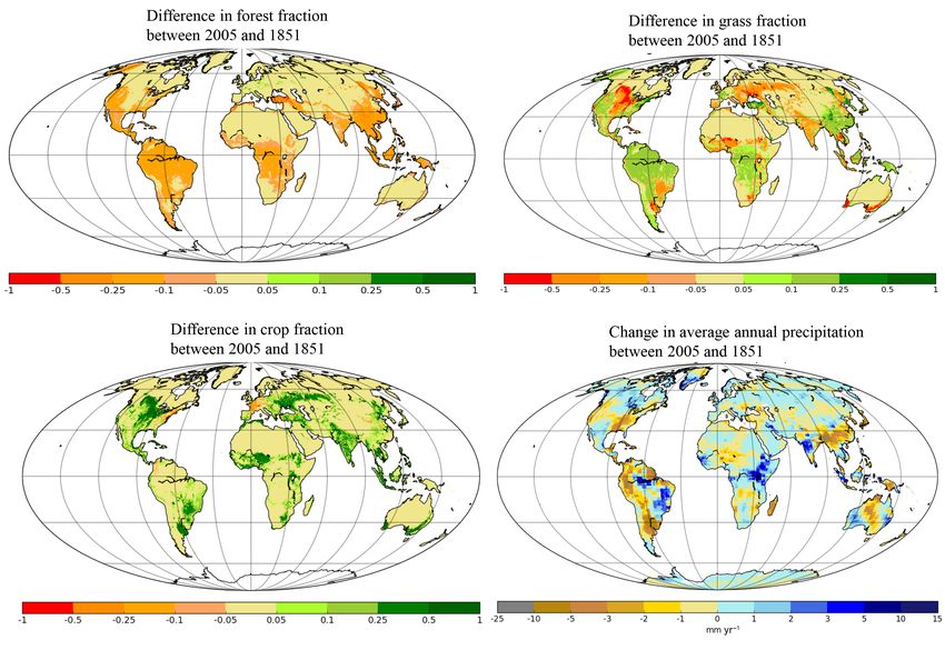
4460                                                    V. Naipal et al.: Global soil organic carbon removal by water erosion

is stabilized and buried for decades to millennia (Hoffmann        carbon dynamics models at different spatial and temporal
et al., 2013a, b; Wang et al., 2017). Together with dynamic        scales. Some studies coupled process-oriented soil erosion
replacement of removed SOC by new litter input at the erod-        models with carbon turnover models calibrated for specific
ing sites, and the progressive exposure of carbon-poor deep        micro-catchments on timescales of a few decades to a mil-
soils, this translocated and buried SOC can lead to a net car-     lennium, (Billings et al., 2010; Van Oost et al., 2012; Nadeu
bon sink at the catchment scale, potentially offsetting a large    et al., 2015; Wang et al., 2015a; Zhao et al., 2016; Bouchoms
part of the carbon emissions from LUC (Berhe et al., 2007;         et al., 2017). Other studies focused on the application of par-
Bouchoms et al., 2017; Harden et al., 1999; Hoffmann et al.,       simonious erosion–SOC-dynamics models using the Revised
2013a; Lal, 2003; Stallard, 1998; Wang et al., 2017).              Universal Soil Loss Equation (RUSLE) approach together
   On eroding sites, soil erosion keeps the SOC stocks below       with sediment transport methods at regional or continental
a steady state (Van Oost et al., 2012) and can lead to substan-    spatial scales (Chappell et al., 2015; Lugato et al., 2016; Yue
tial CO2 emissions in certain regions (Billings et al., 2010;      et al., 2016; Zhang et al., 2014). However, the modeling ap-
Worrall et al., 2016; Lal, 2003). CO2 emission from soil ero-      proaches used in these studies apply erosion models that still
sion can take place during the breakdown of soil aggregates        require many variables and data input that is often not avail-
by erosion and during the transport of the eroded SOC by           able at the global scale or for the past or the future time pe-
runoff and later also by streams and rivers.                       riod. These models also run on a much higher spatial reso-
   LUC emissions are usually quantified using bookkeeping          lution than LSMs, making it difficult to integrate them with
models and LSMs that represent the impacts of LUC activ-           LSMs. The study of Ito (2007) was one of the first studies to
ities on the terrestrial carbon cycle (Le Quéré et al., 2016).     couple water erosion to the carbon cycle at the global scale,
These impacts are represented through processes leading to         using a simple modeling approach that combined the RUSLE
a local imbalance between net primary productivity (NPP)           model with a global ecosystem carbon cycle model. How-
and heterotrophic respiration, ignoring lateral displacement.      ever, there are several unaddressed uncertainties related to his
Currently, LSMs consider only the carbon fluxes following          modeling approach, such as the application of the RUSLE at
LUC resulting from changes in vegetation, soil carbon, and         the global scale without adjusting its parameters.
sometimes wood products (Van Oost et al., 2012; Stocker et            Despite all the differences between the studies that cou-
al., 2014). The additional carbon fluxes associated with the       pled soil erosion to the carbon cycle, they all agree that soil
human action of LUC from the removal and lateral transport         erosion by rainfall and runoff is an essential component of
of SOC by erosion are largely ignored.                             the carbon cycle. Therefore, to better constrain the land–
   In addition, the absence of lateral SOC transport by ero-       atmosphere and the land–ocean carbon fluxes, it is neces-
sion in LSMs complicates the quantification of the human           sary to develop new LSM-compatible methods that explic-
perturbation of the carbon flux from land to inland waters         itly represent the links between soil erosion and carbon dy-
(Regnier et al., 2013). Recent studies have been investigat-       namics at regional to global scales and over long timescales.
ing the dissolved organic carbon (DOC) transfers along the         Based on this, our study introduces a 4-D modeling ap-
terrestrial–aquatic continuum in order to better quantify CO2      proach that consists of (1) an emulator that simulates the car-
evasion from inland waters and to constrain the lateral car-       bon dynamics like in the ORCHIDEE LSM (Krinner et al.,
bon flux from the land to the ocean (Lauerwald et al., 2017;       2005), (2) the Adjusted Revised Universal Soil Loss Equa-
Regnier et al., 2013). They point out that an explicit repre-      tion (Adj.RUSLE) model that has been adjusted to simulate
sentation of soil erosion and transport of particulate organic     global soil removal rates based on coarse-resolution data in-
carbon (POC) – in addition to DOC leaching and transport           put from climate models (Naipal et al., 2015), and (3) a spa-
– in future LSMs is essential to be able to better constrain       tially explicit representation for LUC. This approach repre-
the flux from land to ocean. This is true, since the transfer of   sents explicitly and consistently the links between the pertur-
POC from eroded SOC forms an important part of the carbon          bation of the terrestrial carbon cycle by elevated atmospheric
inputs to rivers.                                                  CO2 and variability (temperature and precipitation change),
   The slow pace of carbon sequestration by soil erosion and       the perturbation of the carbon cycle by LUC, and the effect
deposition (Van Oost et al., 2012; Wang et al., 2017) and          of soil erosion at the global scale.
the slowly decomposing SOC pools require the simulation               The main goal of our study is to use this new modeling
of soil erosion at timescales longer than a few decades to         approach to determine the potential effects of long-term soil
fully quantify its impacts on the SOC dynamics. This, and          erosion by rainfall and runoff without deposition or transport
the high spatial resolution that soil erosion models typically     on the global SOC stocks under LUC, climate variability, and
require, complicates the introduction of soil erosion and re-      increasing atmospheric CO2 levels. In order to be able to de-
lated processes in LSMs that use short time steps (≈ 30 min)       termine if global soil erosion is a net carbon source or sink,
for simulating energy fluxes and require intensive computing       it is essential to study first how soil erosion, without depo-
resources.                                                         sition or transport, interacts with the terrestrial carbon cycle.
   Previous approaches used to explicitly couple soil erosion      Therefore, we also aim to understand the links between the
and SOC turnover have been applying different erosion and          different perturbations to the carbon cycle in the presence of

Biogeosciences, 15, 4459–4480, 2018                                                     www.biogeosciences.net/15/4459/2018/
V. Naipal et al.: Global soil organic carbon removal by water erosion                                                        4461

soil erosion and to identify relevant changes in the spatial      temperature conditions controlling litter and soil carbon de-
variability of SOC stocks under erosion.                          composition over time. All the processes that determine sur-
                                                                  face and soil temperature and soil moisture are calculated by
                                                                  the ORCHIDEE LSM on a 30 min time step. Such a time
2     Materials and methods                                       step is needed for coupled simulations with a climate model
                                                                  but makes the LSM model CPU intensive. However, there
2.1    Modeling framework concept
                                                                  is no need for such high-temporal-resolution calculations
We used the LSM ORCHIDEE-MICT (Guimberteau et al.,                of “fast” carbon and energy fluxes to account for erosion-
2018; Zhu et al., 2016) (in the following simply referred         induced effects on SOC stocks. The addition of erosion is
to as ORCHIDEE) to construct a carbon emulator that de-           here supposed to impact only carbon pools and to have no
scribes the carbon pools and fluxes exactly as in ORCHIDEE        feedbacks on soil moisture, soil temperature, and photosyn-
(Fig. 1a). MICT stands for aMeliorated Interactions between       thesis. Therefore, we decided to use the emulator concept
Carbon and Temperature, and this version of ORCHIDEE              rather than incorporating erosion processes directly into OR-
has several major modifications and improvements for espe-        CHIDEE. For each carbon pool the stock and all the incom-
cially the high latitudes.                                        ing and outgoing fluxes are derived at a daily time step from
   ORCHIDEE has eight biomass pools, four litter pools, of        a single simulation performed with the ORCHIDEE LSM.
which two are aboveground and two are belowground, and            Based on the daily output stock and fluxes, the values of the
three SOC pools for each land cover type (Fig. 1a). It has        turnover rates are calculated and archived together with the
been extensively validated using observations on energy, wa-      input fluxes to build the emulator. Then, the emulator can be
ter, and carbon fluxes at various eddy-covariance sites, and      run to simulate the dynamics of all pools over long timescales
with measurements of atmospheric CO2 concentration (Piao          without having to recompute carbon fluxes at each time step.
et al., 2009). The land cover types are represented by 12 plant   In this way the emulator reduces the computation time of the
functional types (PFTs) and an additional type for bare soil.     complex ORCHIDEE model significantly and allows us to
A total of 10 PFTs represent natural vegetation and 2 repre-      easily add and study erosion-related processes affecting the
sent agricultural land (C3 and C4 crop). The turnover times       carbon dynamics of the soil. Our main objective here is to
for each of the PFT-specific litter and SOC pools depend on       present a tool able to evaluate erosion-related carbon fluxes
their residence time modified by local soil texture, humidity,    at global scale using a state-of-the-art LSM output and to es-
and temperature conditions (Krinner et al., 2005). The loss of    timate the drivers of carbon erosion at the global scale.
biomass and litter carbon by fire is represented by the param-       ORCHIDEE also includes crop harvest, defined as the har-
eterization of the Spitfire model from Thonicke et al. (2011)     vest of aboveground biomass of agricultural PFTs and calcu-
in the full ORCHIDEE model and currently cannot be modi-          lated based on the concept of the harvest index (HI) (Krinner
fied in our version of the emulator. Carbon losses by fire here   et al., 2005). The HI is defined as the yield of crop expressed
are considered to contribute directly to the CO2 emissions        as a fraction of the total aboveground dry matter production
from land.                                                        (Hay, 1995). ORCHIDEE uses a fixed HI for crop of 0.45.
   At face value, the emulator merely copies the ORCHIDEE         However, Hay (1995) showed that the HI has increased sig-
carbon pool dynamics, and for each new atmospheric CO2            nificantly since 1900 for C3 crops such as wheat. In the emu-
and climate scenario a new run of the original LSM is re-         lator, and also in the full ORCHIDEE model, the carbon bal-
quired to build the emulator. The emulator thus reproduces        ance of agricultural lands is sensitive to crop harvest. Based
exactly the carbon pool dynamics of the full LSM. The             on this we use the findings of Hay (1995) to change the HI
change in carbon over time for each pool of the original          of C3 crops to be temporally variable over the period 1850–
model is represented in the emulator by the following gen-        2005 in the emulator, with values ranging between 0.26 and
eral mass-balance approach:                                       0.46. This means that more crop biomass is harvested against
                                                                  what becomes litter. We only changed the HI of C3 plants,
dC                                                                because Hay (1995) mentioned that C4 plants, such as maize,
   = I (t) − k × C(t).                                     (1)    had already a high HI at the start of the last century. It should
dt
                                                                  be noted that the harvest index does not vary spatially in our
Here, dCdt represents the change in carbon stock of a certain     emulator, and harvesting is then done constantly at each time
pool over time, calculated by the difference between the in-      step.
coming flux (I (t)) and the outgoing flux (k × C(t)) to the
respective pool, where k is the turnover rate. Although orig-     2.2   Net land use change
inally calculated by complex equations, the dynamic evolu-
tion of each pool can be described using the first-order model    Land use change is not taken into account in the ORCHIDEE
of Eq. (1). Complex equations, such as photosynthesis and         LSM version we are using in this study to build the emula-
hydrological processes, are needed to simulate realistically      tor, but is represented by a net land use change routine in
the carbohydrate input to carbon pools and the moisture and       the emulator that includes past agricultural land and grass-

www.biogeosciences.net/15/4459/2018/                                                     Biogeosciences, 15, 4459–4480, 2018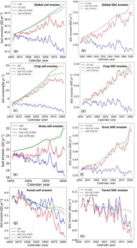
4462                                                      V. Naipal et al.: Global soil organic carbon removal by water erosion

Figure 1. (a) The structure of the carbon emulator (see variable names in the text, Sect. 2.3). The carbon erosion fluxes are represented by
the red arrows and calculated using the soil erosion rates from the Adj.RUSLE model. (b) The land use change module of the emulator.

                                                                         dSOCs (t)
land expansion over natural PFTs (Fig. 1b). This makes it                          = lits (t) + kas × SOCa (t)
possible to switch the LUC routine on or off in the emula-                  dt
tor or to change LUC scenarios when needed without hav-                    − ksa + ksp + k0s × SOCs (t),                                (3)
ing to rerun ORCHIDEE. We verified that the LUC routine                  dSOCp (t)
added to the emulator conserves the mass of all carbon pools                       = kap × SOCa (t) + ksp × SOCs (t)
                                                                            dt
for lands in transition to a new land use type. When LUC                   − (kpa + k0p ) × SOCp (t),                                   (4)
takes place, the fractions of PFTs in each grid cell are up-
dated every year given prescribed annual maps of agricul-               where SOCa , SOCs , and SOCp (g C m−2 ) are the active (un-
tural and natural PFTs (Peng et al., 2017). The carbon stocks           protected); slow (physically or chemically protected); and
of the litter and SOC pools of all the shrinking PFTs are               passive (biochemically recalcitrant) SOC, respectively. The
then summed and allocated proportionally to the expanding               SOC pools are based on the study of Parton et al. (1987) and
or new PFTs, maintaining the mass balance (Houghton and                 are defined by their residence times. The active SOC pool
Nassikas, 2017; Piao et al., 2009). When natural vegetation is          has the lowest residence time (∼ 1.5 years) and the passive
reduced by LUC, the heartwood and sapwood biomass pools                 the highest (∼ 1000 years). lita and lits (g C m−2 day−1 ) are
are harvested and transformed to three wood products with               the litter input rates to the active and slow SOC pools, re-
turnover times of 1, 10 and 100 years. The other biomass                spectively; k0a , k0s , and k0p (day−1 ) are the respiration rates
pools (leafs, roots, sapwood belowground, fruits, heartwood             of the active, slow, and passive pools, respectively; kas , kap ,
belowground) are transformed to metabolic or structural lit-            kpa , ksa , ksp are the coefficients determining the flux from the
ter and allocated to the respective litter pools of the expand-         active to the slow pool, from the active to the passive pool,
ing PFTs (Piao et al., 2009).                                           from the passive to the active pool, from the slow to the ac-
                                                                        tive pool, and from the slow to the passive pool, respectively
2.3    Soil carbon dynamics                                             (Fig. 1a).
                                                                           The SOC pools are not vertically discretized in the ver-
The change in the carbon content of the PFT-specific SOC                sion of the ORCHIDEE LSM used to build the emulator,
pools in the emulator without soil erosion can be described             so we implemented a simple vertical discretization scheme
with the following differential equations:                              for the SOC pools in the emulator based on the concept of
                                                                        Wang et al. (2015a, b). In this scheme the carbon dynamics
                                                                        of each soil layer are calculated separately, based on layer-
dSOCa (t)                                                               dependent litter input and respiration rates (Fig. 1a). The ver-
          = lita (t) + kpa × SOCp (t) + ksa × SOCs (t)
   dt                                                                  tical discretization scheme of the emulator does not change
  − kap + kas + k0a × SOCa (t),                                (2)      the total input and respiration as simulated by ORCHIDEE

Biogeosciences, 15, 4459–4480, 2018                                                           www.biogeosciences.net/15/4459/2018/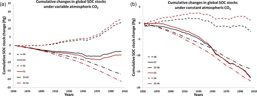
V. Naipal et al.: Global soil organic carbon removal by water erosion                                                            4463

in the case where erosion and land use change processes are         The homogeneously distributed belowground litter input
switched off. We apply the same scheme for all three SOC            (Ibe ) to the layers of the topsoil is equal to
pools, assuming that each SOC pool is equally distributed
                                                                    z=10
across all layers of the soil profile, while the ratios between     X
the pools per soil layer are equal to those from ORCHIDEE.                 I0be × e−r×z × 0.1.                                    (7a)
                                                                    z=0
We base this assumption on the fact that there is very little in-
formation or data to constrain the pool ratios globally, mainly     The belowground litter input to the layers of the subsoil is
because the three SOC pools cannot be directly related to           equal to
measurements (Elliott et al., 1996). Furthermore, neither the
emulator nor the ORCHIDEE LSM model we used include                 Ibe (z) = I0be × e−r×z ,                                      (7b)
soil processes that may affect these pool ratios with depth,
such as vertical mixing by soil organisms, diffusion, leach-        where zmax is the maximum soil depth equal to 2 m and dz
ing, changes in soil texture (SOC protection and stabilization      is the soil layer discretization (1 cm); r is the PFT-specific
by clay particles), and limitations by oxygen and by access         vertical root-density attenuation coefficient as used in OR-
to deep organic matter by microbes. It is also uncertain how        CHIDEE.
sensitive SOC is to these processes. For example, the study            The SOC respiration rates of ORCHIDEE are determined
of Huang et al. (2018), who implemented a matrix-based ap-          by soil temperature, moisture, and texture. In the emulator
proach to assess the sensitivity of SOC, showed that equilib-       we conserve the total respiration of ORCHIDEE (when LUC
rium SOC stocks are more sensitive to input than to mixing          or erosion is absent) and assume that the respiration is homo-
for soils in the temperate and high-latitude regions.               geneously distributed across the layers of the topsoil. For the
    In the vertical discretization scheme of the emulator, the      rest of the soil profile the respiration rates of all three SOC
soil profile is divided into thin layers of 1 cm thickness down     pools decrease exponentially with depth:
to a depth of 2 m, which is the soil depth used by ORCHIDEE
to calculate SOC. The first 10 cm of the soil profile are re-       ki (z) = k0 i × e−re z .                                       (8)
ferred to as the “topsoil”, where we assume that the SOC con-
                                                                    Here k0 i is the SOC respiration rate at the surface layer for
tent is homogeneously distributed. The rest of the soil profile
                                                                    each SOC pool (i = a, s, p), and re (m−1 ) is a coefficient rep-
is referred to as the subsoil. The topsoil receives carbon from
                                                                    resenting the impact of external factors, such as oxygen avail-
above- and belowground litter, which is homogeneously dis-
                                                                    ability, which reduce SOC mineralization rate with depth (z).
tributed across the soil layers of the topsoil.
                                                                    To ensure that the total soil respiration of the emulator is sim-
    The belowground litter input for the active SOC pool is
                                                                    ilar to that of the ORCHIDEE LSM model for each grid cell,
the sum of a fraction of the belowground structural and
                                                                    each PFT, and each SOC pool, we have calibrated the ex-
metabolic litter pools of ORCHIDEE being recalculated by
                                                                    ponent “re ” and variable “k0i ” of Eq. (8) for each grid cell
the emulator to change with depth, while the belowground
                                                                    and PFT under equilibrium conditions. First we selected a
litter input for the slow SOC pool is equal to a fraction of the
                                                                    default value for re between 0 and 5 and calculated the respi-
belowground structural litter pool only. This setting is consis-
                                                                    ration rate of the surface soil layer (k0 ) when all SOC pools
tent with the structure of the SOC module of the ORCHIDEE
                                                                    are in an equilibrium state, with the following equation:
LSM to ensure that the emulator reproduces the same C pool
dynamics as the LSM. The litter fractions are based on the                           Xz=n          L (z)
Century model as introduced by Parton et al. (1987) and             SOCorchidee =        z=0 k0 × e−re ×z
                                                                                                            ,                      (9)
later implemented inside ORCHIDEE (Krinner et al., 2005).
We assume that the subsoil receives carbon only from be-            where SOCorchidee is the total equilibrium SOC stock derived
lowground litter and that this input decreases exponentially        from ORCHIDEE for a certain grid cell and PFT. L(z) is the
with depth following the root profile of ORCHIDEE. This             total litter input to the soil for a certain soil layer discretized
discretization of the total belowground litter input (litbe ) is    according to the root profile. Then we derived the equilib-
the same for both SOC pools and can then be represented as          rium SOC stocks per soil layer as
                                                                                     L (z)
          Z   z=zmax                                                SOC (z) =                  .                                  (10)
litbe =                I0be × e   −r×z
                                         dz,                 (5)                  k0 × e−re ×z
          z=0
                                                                    Assuming that the ratios between the active, slow, and pas-
                                                                    sive SOC pools do not change with depth and are equal to
where I0be is the belowground litter input to the surface layer
                                                                    the ratios derived from ORCHIDEE, we calculated the SOC
and is equal to
                                                                    stocks of each pool with the following equation:

                           r                                               soils (z) soilp (z) SOC (z)
I0be = litbe ×                       .                       (6)    1+              +          =           ,                      (11)
                  1 − e−r×zmax                                             soila (z) soila (z)   soila (z)

www.biogeosciences.net/15/4459/2018/                                                           Biogeosciences, 15, 4459–4480, 2018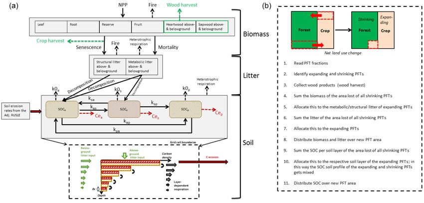
4464                                                     V. Naipal et al.: Global soil organic carbon removal by water erosion

where soila (z), soils (z), and soilp (z) are the emulator-derived   where       R     is    the      rainfall     erosivity     factor
active, slow, and passive SOC stocks per soil layer, grid cell,      (MJ mm ha−1 h−1 year−1 ), K is the soil erodibility fac-
and PFT. Now, for the equilibrium state the input is equal to        tor (t ha h ha−1 MJ−1 mm−1 ), C is the land cover factor
the output, allowing us to derive k0a , k0s , and k0p with the       (dimensionless), and S is the slope steepness factor (di-
following equations:                                                 mensionless). The S factor is calculated using the slope
                                                                     from a 1 km resolution digital elevation model (DEM) that
Xz=n  La (z) + ksa × soils (z) + kpa × soilp (z)                   has been scaled using the fractal method to a resolution
   z=0            k0a × e−re ×z + kas + kap                          of 150 m (Naipal et al., 2015). In this way the spatial
 = SOCa ,                                                   (12a)    variability of a high-resolution slope dataset can be captured.
Xz=n  Ls (z) + kas × soila (z)                                     The computation of the R factor has been adjusted to
                                   = SOCs ,                 (12b)    use coarse-resolution input data on precipitation and to
   z=0 k0s × e−re ×z + ksa + ksp                                     provide reasonable global erosivity values. For this Naipal et
Xz=n  ksp × soils (z) + kap × soila (z)                            al. (2015) derived regression equations for different climate
                                           = SOCp ,         (12c)
 z=0         k0p × e−re ×z + kpa                                     zones of the Köppen–Geiger climate classification (Peel et
                                                                     al., 2007). The results from the Adj.RUSLE model have
where La is the total litter input to the active SOC pool            been tested against empirical large-scale assessments of soil
and Ls is the total litter input to the slow SOC pool. SOCa ,        erosion and rainfall erosivity (Naipal et al., 2015, 2016). The
SOCs , and SOCp are the total active, slow, and passive SOC          original RUSLE model as described by Renard et al. (1997)
stocks per grid cell and PFT, respectively, derived from OR-         also includes the slope-length (L) and support-practice
CHIDEE. kas , kap , ksa , ksp , kpa are the coefficients determin-   (P ) factors. Although these factors can strongly affect soil
ing the fluxes between the SOC pools. After the derivation           erosion in certain regions, the Adj.RUSLE does not include
of k0i we tested if the difference in the SOC stocks between         these factors due to several reasons. Firstly, Doetterl et
the emulator and the original ORCHIDEE LSM is less than              al. (2012) showed that these factors do not significantly
1 g m−2 per grid cell and PFT. If this was not the case we           contribute to the variation in soil erosion at the continental
increased or decreased the value of “re ” and repeated the cal-      to global scales, in comparison to the other RUSLE factors.
ibration cycle. If we did not find an optimized value for both       Secondly, data on the L and P factors and methods to
re and k0i that meet this criteria, we used values that min-         estimate them at the global scale are very limited. Thus,
imized the difference in SOC stocks between the emulator             including them in global soil erosion estimations would
and the original ORCHIDEE LSM.                                       result in large uncertainties. Finally, the focus of this study is
   For the transient period (without LUC or erosion) we as-          to show the effects of potential soil erosion on the terrestrial
sumed a time-constant re , where the values are equal to those       carbon cycle, without the explicit effect of management
at equilibrium. Using the mass-balance approach we calcu-            practices such as covered by the P factor. For more infor-
lated the daily values for k0a , k0s , k0p per grid cell and PFT     mation on the validation of our erosivity values and a more
with                                                                 detailed description of the calculation of each of the RUSLE
                                                                     factors see Supplement Sect. S1.
dSOCa Xz=n
       =           (La (z, t)                                           The Adj.RUSLE model is not imbedded in the C emulator
  dt           z=0
                                                                     but is run separately on a 5 arcmin spatial resolution and at a
  + ksa × soils (z, t − 1) + kpa × soilp (z, t − 1)                  yearly timestep. The resulting soil erosion rates are then read
  − k0a (t) × e−re ×z + kas + kap × soila (z, t − 1) , (13a)

                                                                     by the C emulator at each time step and used to calculate
dSOCs Xz=n                                                           the daily SOC erosion rate of a certain SOC pool i (Cei in
       =      z=0
                   (Ls (z, t) + kas × soila (z, t − 1)               g C m−2 day−1 ) at the surface layer by
  dt
  − k0s (t) × e−re ×z + ksa + ksp × soils (z, t − 1) , (13b)

                                                                                           E
                                                                                          365   × 100
dSOCp Xz=n                                                           Cei = SOCi ×                        ,                        (15)
        =           k × soils (z, t − 1)                                             BDtop × dz × 106
  dt           z=0 sp
  + kap × soila (z, t − 1) − k0p (t) × e−re ×z + kpa

                                                                     where BDtop is the bulk density of the surface layer (g cm−3 ).
                                                                     We assume that the enrichment ratio, i.e., the volume ratio of

  ×soilp (z, t − 1) .                                     (13c)
                                                                     the carbon content in the eroded soil to that of the source soil
In case there was no solution for the k0i at a certain time step     material, is equal to 1 here, which implies that our estimates
we took the values from the previous time step.                      of SOC mobilization are likely conservative (Chappell et al.,
   The annual average soil erosion rate (E, t ha−1 year−1 ) is       2015; Nadeu et al., 2015).
calculated by the Adj.RUSLE (Naipal et al., 2015, 2016) ac-             When erosion takes place, the surface layer is truncated by
cording to                                                           the erosion height, and at the same time an amount of SOC
                                                                     corresponding to this erosion height is removed. As we as-
E = S × R × K × C,                                           (14)    sume that the soil layer thickness does not change, part of

Biogeosciences, 15, 4459–4480, 2018                                                       www.biogeosciences.net/15/4459/2018/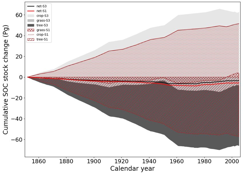
V. Naipal et al.: Global soil organic carbon removal by water erosion                                                        4465

the SOC of the next soil layer is allocated to the surface layer   Phase 5 (CMIP5 output of IPSL-CM5A-LR (Taylor et al.,
proportional to the erosion height and the SOC concentration       2012), which are bias corrected using observational datasets
(per volume) of the next layer. In this way, SOC from all the      and the method of Hempel et al. (2013) and made available
following soil layers moves upward and becomes exposed to          at a resolution of 0.5◦ (Fig. 2). We chose these data as input
erosion in the surface layer at some point in time (Fig. 1a). To   to the Adj.RUSLE model, because the dataset extended to
preserve mass balance, we assume that there is no SOC be-          1850, in contrast to the CRU-NCEP data. Also, this dataset
low the 2 m soil profile represented in the emulator and new       being bias corrected provides a better distribution of extreme
substrate replacing the material of the last soil layer is SOC     events and frequencies of dry and wet days (Frieler et al.,
free, so that SOC in the bottom layer will decrease towards        2017), which is important for the calculation of rainfall ero-
zero after erosion has started.                                    sivity (R factor). The ISIMIP precipitation data were regrid-
                                                                   ded using the bilinear interpolation method to the resolution
2.4     Input datasets                                             of the Adj.RUSLE model, before being used to calculate the
                                                                   R factor. This was necessary because the erosivity equations
2.4.1    For ORCHIDEE                                              from the Adj.RUSLE model are calibrated at this specific res-
                                                                   olution (Naipal et al., 2015).
We used 6-hourly climate data supplied by the CRU-NCEP                Data on soil bulk density and other soil parameters to cal-
(version 5.3.2) global database (https://crudata.uea.ac.uk/        culate the soil erodibility factor (K), available at the resolu-
cru/data/ncep/; last access: 16 July 2018) available at 0.5◦       tion of 1 km, have been taken from the Global Soil Dataset
resolution to perform simulations with the full ORCHIDEE           for use in Earth System Models (GSDE) (Shangguan et al.,
model for constructing the emulator. CRU-NCEP climate              2014). The K factor has been calculated at the resolution of
data were only available for the period 1901–2012. To be           1 km before being regridded to 5 arcmin using the bilinear
able to run ORCHIDEE for the period 1850–1900, we ran-             interpolation method. We also used the SOC concentration
domly projected the climate forcing after 1900 to the years        in the soil from GSDE, which was derived using the “aggre-
before 1900. The random projection of the climate data is          gating first” approach, to compare to our SOC stocks from
necessary to avoid the risk of including the effects of extreme    simulations with the emulator. Finally, the slope steepness
climate conditions multiple times when only a certain decade       factor (S), which was originally estimated at the resolution
is used repeatedly.                                                of 1 km, was also regridded to the resolution of 5 arcmin us-
   The historical changes in PFT fractions were derived from       ing the bilinear interpolation method.
the historical annual PFT maps of Peng et al. (2017). These           Using the above-mentioned data, soil erosion rates were
PFT maps were available at a resolution of 0.25◦ (Fig. 2) and      first calculated at the resolution of 5 arcmin and afterwards
were regridded to the resolution of the ORCHIDEE emulator,         aggregated to the coarse resolution of the emulator (2.5◦ ×
which is 2.5 × 3.75, using the nearest-neighbor approach.          3.75◦ ) to calculate daily SOC erosion rates.

2.4.2    For the Adj.RUSLE                                         2.5   Model simulations

Due to the resolution of the Adj.RUSLE, which is 5 arcmin          To be able to understand and estimate the different direct and
(∼ 0.0833◦ ), all the RUSLE factors had to be regridded or         indirect effects of soil erosion on the SOC dynamics, we pro-
calculated at this specific resolution before calculating the      pose a factorial simulation framework (Fig. 3 and Table 1).
soil erosion rates.                                                This framework allows isolating or combining the main pro-
   The land cover fractions from the historical 0.25◦ PFT          cesses that link soil erosion to the SOC pool, namely the in-
maps were used in combination with the LAI values from             fluence from climate variability, LUC, and atmospheric CO2
ORCHIDEE at the resolution of 2.5◦ × 3.75◦ to derive the           increase. The different model simulations described in this
values for the C factor of the RUSLE model. We first regrid-       section will be based on this framework.
ded the yearly average LAI to the resolution of the PFT maps          We performed two different simulations with the full OR-
before calculating the land cover factor of RUSLE (C factor)       CHIDEE model to produce the required data input for the
at the resolution of 0.25◦ . The C values were then regridded      emulator for the period 1850–2005. For this we first per-
using the nearest-neighbor method to the resolution of the         formed a spinup with ORCHIDEE to get steady-state car-
Adj.RUSLE model. We used the nearest-neighbor approach             bon pools for the year 1850. We chose the period 1850–2005
here, because the C factor is strongly dependent on the land       based on the ISIMIP2b precipitation data availability and the
cover class.                                                       fact that this period underwent a significant intensification
   Daily precipitation data for the period 1850–2005 to cal-       in agriculture globally and a substantial rise in atmospheric
culate soil erosion rates is derived from the Inter-Sectoral       CO2 concentrations. In the first simulation of ORCHIDEE
Impact Model Intercomparison Project (ISIMIP), product             the global atmospheric CO2 concentration was fixed to the
ISIMIP2b (Frieler et al., 2017). These data are based on           year 1850 to calculate time-varying NPP not impacted by
model output of the Coupled Model Intercomparison Project          CO2 fertilization and subsequent carbon pools, while in the

www.biogeosciences.net/15/4459/2018/                                                      Biogeosciences, 15, 4459–4480, 2018
4466 V. Naipal et al.: Global soil organic carbon removal by water erosion
Figure 2. Spatial patterns of the difference in forest, crop, and grassland area between 1851 and 2005 represented as a fraction of a grid
cell. And spatial patterns of the change in average annual precipitation between 1851 and 2005 in mm yr−1 , calculated as the total change in
precipitation over the period 1850–2005 and divided by the number of years in this period.
second simulation the atmospheric CO2 concentration was lator to perform eight main simulations and four sensitivity
made variable. In both simulations, climate is variable and simulations. The different simulations and their description
derived from CRU-NCEP (Fig. 3). are given in Table 1 and Fig. 3. In the simulations without
Furthermore, we performed seven simulations with the LUC (S2, S4, S6, and S8), the PFT fractions and the harvest
Adj.RUSLE model to precalculate the soil erosion rates that index are constant and equal to those in the year 1850. In the
will be used as input to the ORCHIDEE emulator. Three of simulations with LUC (S1, S3, S5, and S7) the harvest in-
the seven erosion simulations used best estimates for each dex increases and the PFT fraction changes with time during
model parameter, and the rest used either the minimum or 1850–2005. In each emulator simulation we first calculated
maximum values for the R and C factors to derive an un- the equilibrium carbon stocks analytically before calculating
certainty range for our soil erosion rates and to analyze the the change in the carbon stocks in time depending on the per-
sensitivity of the emulator. In the first simulation with the turbations during the transient period (1851–2005). In simu-
best estimated model parameters we kept the climate and lations with erosion, the equilibrium state of the SOC pools
land cover variable through time (the “CC + LUC” simula- has been calculated using the average erosion rates of the
tion). In the second simulation we only varied the climate period 1850–1859, assuming erosion to be constant before
through time and kept land cover fractions fixed to 1850 (the 1850 and a steady-state condition where erosion fluxes are
“CC” simulation, Fig. 3). In the third simulation we only var- equal to input from litter.
ied the land cover through time and kept the climate constant
to the average cyclic variability of the period 1850–1859 (the
“LUC” simulation, Fig. 3).The erosion simulations with ei- 3 Results
ther minimum or maximum model parameters were either a
CC + LUC or a CC type of simulation. 3.1 Erosion versus no erosion
From the two simulations of ORCHIDEE (with variable
and constant CO2 ) and the seven soil erosion simulations of After including soil erosion in the ORCHIDEE emulator we
the Adj.RUSLE, we constructed four versions of the emu- obtain a total global soil loss flux of 47.6 ± 10 Pg C year−1
for the year 2005, of which 20 % to 29 % is attributed to
Biogeosciences, 15, 4459–4480, 2018 www.biogeosciences.net/15/4459/2018/V. Naipal et al.: Global soil organic carbon removal by water erosion 4467
Figure 3. Conceptual diagram of SOC affected by erosion in the presence of other perturbations of the carbon cycle, namely climate
variability, increasing atmospheric CO2 concentrations, and land use change. A separation of these components and of the role of erosion is
obtained with the factorial simulations (S1–S8), presented in Table 1.
Table 1. Description of the simulations used in this study. The S1 0.14 Pg C year−1 , of which 26 % to 33 % is attributed to agri-
simulation is also the control simulation (CTR). S1 and S2 mini- cultural land and 54 % to 64 % to grassland (CTR, Fig. 4).
mum and maximum are the sensitivity simulations using minimum Grassland and agricultural land thus have much larger an-
or maximum soil erosion rates. “Best” stands for the best estimated nual average soil and SOC erosion rates compared to forest
soil erosion rates using optimal values for the R and C factors of (Table 2).
the Adj.RUSLE model.
The total soil and SOC losses in the year 2005 show an
increase of 11 %–19 % and 23 %–35 %, respectively, com-
Simulation Climate CO2 Land use Erosion
change change change
pared to 1850 (CTR, Fig. 4), with the largest increases found
in the tropics (Fig. 5b, d). The largest increase in soil and
S1 Yes Yes Yes Best SOC erosion during 1850–2005 is found in South America
S1 minimum Yes Yes Yes Minimum
(Table 3) despite the significant decreases in simulated pre-
S1 maximum Yes Yes Yes Maximum
S2 Yes Yes No Best cipitation leading to less intense erosion rates in this region.
S2 minimum Yes Yes No Minimum One should keep in mind that, due to uncertainties in the sim-
S2 maximum Yes Yes No Maximum ulated LUC and climate variability for certain regions and the
S1–S2 No Yes Yes Best assumptions made in our modeling framework, these trends
S3 Yes Yes Yes No in soil and SOC erosion rates are linked to some uncertainty.
S4 Yes Yes No No However, it is difficult to assess this uncertainty, mainly due
S3–S4 No Yes Yes No
to the lack of observations for the past in regions such as the
S5 Yes No Yes Best
S6 Yes No No Best tropics and the lack of model testing in these regions.
S5–S6 No No Yes Best We found that the total soil erosion flux on agricultural
S7 Yes No Yes No land increased by 55 %–58 % in the year 2005 compared to
S8 Yes No No No 1850, while the SOC erosion flux increased by 11 %–70 %
S7–S8 No No Yes No (Fig. 4) and led to a cumulative SOC removal of 22 ± 5 Pg C
(CTR). On grassland the soil erosion flux increased only by
8 %–20 %, while the SOC erosion flux increased by 44 %–
54 % (Fig. 4) and led to a cumulative SOC mobilization of
agricultural land and 51 % to 55 % to grassland. This global 38 ± 7 Pg C since 1850. It is evident that on agricultural land
soil loss flux (here “loss” meaning horizontal removal of the uncertainty range of soil erosion leads to a large uncer-
SOC by erosion) leads to a total SOC loss flux of 0.52 ±
www.biogeosciences.net/15/4459/2018/ Biogeosciences, 15, 4459–4480, 20184468 V. Naipal et al.: Global soil organic carbon removal by water erosion Figure 4. (a) Global annual soil erosion rates, (b) global annual SOC erosion rates, (c) agricultural annual soil erosion rates, (d) agricultural annual SOC erosion rates, (e) grassland annual soil erosion rates, (f) grassland annual SOC erosion rates, (g) forest annual soil erosion rates, and (h) forest annual SOC erosion rates over the period 1850–2005 for scenarios with only LUC (green lines), the scenario with only climate and CO2 change (blue line), and the scenario with LUC, climate, and CO2 change (red line). In (a), (c), (e), and (g) the dashed green line is the difference between the CTR and S2 simulations, while the straight green line is the LUC-only simulation with the Adj.RUSLE model. Biogeosciences, 15, 4459–4480, 2018 www.biogeosciences.net/15/4459/2018/
V. Naipal et al.: Global soil organic carbon removal by water erosion                                                                              4469

Table 2. Area-weighted average and standard deviation of soil and SOC erosion rates per land cover type for the year AD 2005; the uncer-
tainty range for soil erosion rates is 25 %–53 % and for SOC erosion rates 16 %–50 %.

                         PFT                                        Standard                                         Standard
                                          Mean soil                deviation               Mean SOC                 deviation
                                            erosion              soil erosion                 erosion             SOC erosion
                                    (t ha−1 year−1 )        (t ha−1 year−1 )       (kg C ha−1 year−1 )     (kg C ha−1 year−1 )
                         Crop                   2.45                      35                    10.38                     466
                         Grass                  1.80                      30                     5.79                      91
                         Forest                 0.34                       3                     1.34                      14

Table 3. Model estimates per continent of area-weighted average annual soil erosion and SOC erosion rates for the year 2005, their spatial
standard deviations, and the changes in average soil and SOC erosion rates since 1851; the uncertainty range for soil and SOC erosion rates
is 2 %–36 % and 3 %–52 %, respectively. The uncertainty range for the changes in soil and SOC erosion rates since 1851 is 3 %–83 % and
11 %–166 %, respectively.

   Region                                       Standard                                                             Standard
                                               deviation             Change in                                      deviation             Change in
                           Mean soil         soil erosion             mean soil             Mean SOC              SOC erosion             mean SOC
                         erosion rate                rate           erosion rate            erosion rate                  rate           erosion rate
                               2005                 2005            2005–1851                     2005                   2005            2005–1851
                    (t ha−1 year−1 )    (t ha−1 year−1 )       (t ha−1 year−1 )     (kg C ha−1 year−1 )    (kg C ha−1 year−1 )   (kg C ha−1 year−1 )
   Africa                       2.35              59.96                   0.58                    13.19                 95.22                   4.31
   Asia                         5.66             157.90                   0.21                    58.03                802.53                   3.23
   Europe                       2.07              62.50                   0.39                    16.68                338.03                   1.39
   Australia                    1.40              16.29                  −0.47                     5.16                 22.91                   1.82
   South America                4.52             113.26                   1.29                    74.42               1515.04                  38.97
   North America                2.60              58.62                   0.13                    32.88                556.44                   3.14
   Global                       3.61              96.43                   0.45                    38.56                666.39                   8.94

tainty range in SOC erosion compared to grassland. The in-                         total SOC stock of 1001 ± 58 Pg C for the year 2005 (Ta-
crease in SOC erosion is much larger than the increase in soil                     ble 5). We also find that including soil erosion in the SOC-
erosion for grasslands because in our model LUC (without                           dynamics scheme slightly improves the root mean square er-
erosion) leads to a significant increase in SOC on grassland                       ror (RMSE) between the simulated SOC stocks and those
amplifying the increasing trend in SOC erosion for grass-                          from GSDE for the top 30 cm of the soil profile. This im-
land. This simulated increase in SOC stocks on grasslands                          provement in the RMSE occurs especially in highly erosive
after LUC is not unrealistic, as it is observed from paired                        regions. Furthermore, the total SOC stock of agricultural land
chronosequences worldwide where grasslands have higher                             is significantly lower than that of the GSDE, because we as-
SOC densities than forests, for instance (Li et al., 2017).                        sume a steady-state landscape at 1850, where soil erosion
   In total 7183 ± 1662 Pg of soil and 74 ± 18 Pg of SOC is                        losses are equal to the carbon input to the soil. We did not
mobilized across all PFTs by erosion during the period 1850–                       perform a more in-depth comparison with SOC global obser-
2005, which is equal to approximately 46 %–74 % of the total                       vations as our emulator and the original ORCHIDEE LSM
net flux of carbon lost as CO2 to the atmosphere due to LUC                        do not include various soil processes that have been proven
(net LUC flux) over the same period estimated by our study                         to affect SOC substantially such as vertical mixing, diffu-
(S1–S2). In this study, we do not address the fate of this large                   sion, priming, changes in soil texture, and carbon-rich or-
amount of eroded SOC, be it partly sequestered (Wang et al.,                       ganic soils formation. The ORCHIDEE LSM model we use
2017) or released to the atmosphere as CO2 .                                       to build the emulator also lacks processes such as nitrogen
                                                                                   and phosphorus limitations, which affect the productivity and
3.2   Validation of model results                                                  SOC decomposition (Goll et al., 2017; Guenet et al., 2016).
                                                                                   The emulator also simulates only the removal of SOC but
We calculated a total global SOC stock for the year 2005                           not the subsequent SOC transport and deposition after ero-
in the absence of soil erosion (S3) of 1284 Pg C, which is a                       sion, and there is a general uncertainty in the simulation of
factor of 0.73 lower than the total SOC stock from GSDE                            underlying processes that govern the SOC dynamics (Todd-
(Shangguan et al., 2014) for a soil depth of 2 m (Table 5).                        Brown et al., 2014). Finally, large uncertainties in the global
Including soil erosion (S1, minimum, maximum) leads to a

www.biogeosciences.net/15/4459/2018/                                                                         Biogeosciences, 15, 4459–4480, 2018
4470 V. Naipal et al.: Global soil organic carbon removal by water erosion
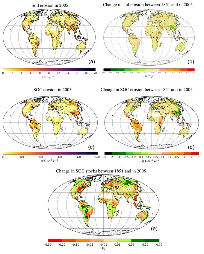
Figure 5. (a) Average annual soil erosion rates at a 5 arcmin resolution in the year 2005, (b) change in average annual soil erosion rates
over the period 2005–1850, (c) average annual SOC erosion rates at a resolution of 2.5 × 3.75◦ in 2005, (d) change in average annual SOC
erosion rates over the period 2005–1850, and (e) difference in SOC stocks at a resolution of 2.5 × 3.75◦ between the year 2005 and 1850
(CTR simulation). For the SOC stocks positive values (green color) indicate a gain, while negative values (red color) indicate a loss. For the
erosion rates positive values (red color) indicate an increase over 1850–2005, while negative values (green color) indicate a decrease over
1850–2005.
soil databases (Hengl et al., 2014; Scharlemann et al., 2014; Using the Adj.RUSLE model to estimate agricultural soil
Tifafi et al., 2018) complicate the exact quantification of the loss by water erosion for the year 2005 resulted in a global
uncertainties of the resulting SOC dynamics simulated by our soil loss flux of 12.28 ± 4.62 Pg year−1 (Fig. 4). This flux
emulator. is paralleled by a SOC loss flux of 0.16 ± 0.06 Pg C year−1
after including soil erosion in the CTR simulation (Fig. 4).
Biogeosciences, 15, 4459–4480, 2018 www.biogeosciences.net/15/4459/2018/V. Naipal et al.: Global soil organic carbon removal by water erosion 4471
Table 4. Model estimates per continent of changes in SOC stocks since 1851 from simulations S1, S2, S1–S2, S3, S4, and S3–S4.
Region Change Change Change Change Change Change
SOC stocks SOC stocks SOC stocks SOC stocks SOC stocks SOC stocks
S1 S2 S1–S2 S3 S4 S3–S4
Pg C Pg C Pg C Pg C Pg C Pg C
Africa −1.55 −0.24 −1.31 −1.54 −0.55 −0.98
Asia −0.36 7.94 −8.31 0.65 7.11 −6.47
Europe −3.33 1.78 −5.12 −4.35 1.52 −5.87
Australia 0.21 0.05 0.16 0.29 0.01 0.28
South America 2.24 2.82 −0.59 3.75 2.06 1.69
North America −2.62 3.19 −5.81 −2.5 3.03 −5.53
Global −5.35 15.93 −21.29 −3.3 13.86 −17.16
Table 5. Statistics of a grid cell by grid cell comparison of global SOC stocks between GSDE soil database and simulations S1 (with erosion)
and S3 (without erosion). RMSE is the root mean square error and r value is the correlation coefficient of the linear regression between
GSDE and S1 or S3.
Soil GSDE S1 S3 RMSE RMSE r value r value
depth SOC total SOC total SOC total S1 S3 S1 S3
(m) (Pg) (Pg) (Pg)
0.3 670 428 556 5218 5861 0.43 0.44
1 1356 672 846 14 077 10 213 0.52 0.51
2 1748 1001 1284 12 968 13 195 0.56 0.55
This soil loss flux is in the same order of magnitude as ear- 4 Discussions
lier high-resolution assessments of this flux, while the SOC
removal flux is slightly lower compared to previously pub- 4.1 Significance of including soil erosion in the
lished high-resolution estimates, but within the uncertainty ORCHIDEE emulator
(Table 6). We also find a fair agreement between our model
estimates of recent agricultural soil and SOC erosion fluxes To estimate the net effect of soil erosion on the global SOC
per continent and the high-resolution estimates (excluding stocks under all perturbations we compare the cumulative
tillage erosion) from the study of Doetterl et al. (2012) (Ta- SOC stock change from simulation S3 (no erosion; Table 1)
ble 7). However, the continental SOC erosion fluxes from our with that of the CTR simulation with all factors included, that
study are generally lower, because of the lower SOC stocks is, land use, CO2 , and climate. When considering our best es-
on agricultural land. Only South America shows a higher timated soil erosion rates and assuming that the SOC mobi-
SOC flux for the present day compared to the high-resolution lized by soil erosion in the CTR simulation is all respired, we
estimates of Doetterl et al. (2012), which is the result of the find an overall global SOC stock decrease that is 62 % larger
simulated high productivity of crops in the tropics. compared to a world without soil erosion during the period
Furthermore, we find a cumulative soil loss of 1888 ± 1850–2005 (Fig. 6a). This assumption is certainly an extreme
753 Pg and cumulative SOC removal flux of 22±5 Pg C from and unrealistic assumption, as in reality a fraction of the mo-
agricultural land over the entire time period (CTR simula- bilized SOC will remain stored on land, but we take this as-
tion). This soil loss flux lies in the range of 2480 ± 720 Pg sumption as an extreme scenario. Including soil erosion in
found by Wang et al. (2017) for the same time period, the SOC cycling scheme under the previously mentioned as-
while the SOC removal flux is significantly lower than the sumption thus reduces the global land C sink, with the largest
63±19 Pg C found by Wang et al. (2017). Wang et al. (2017) impact observed for Asia, where the decrease in the total
used only recent climate data in his study while we explicitly SOC stock is 156 % larger when the effects of soil erosion
include the effects of changes in precipitation and tempera- are taken into account (Table 4, Fig. 8a). Some regions, such
ture on global soil erosion rates and the SOC stocks in our as Western Europe show instead a smaller SOC loss when
study, which may partly explain this difference. erosion is taken into account. This is because we assumed
a steady state in 1850, where carbon losses by erosion are
equal to the carbon input by litter. And as soil erosion de-
creased during 1850–2005 in Western Europe – mainly due
to a decreasing trend in precipitation since 1965, less intense
www.biogeosciences.net/15/4459/2018/ Biogeosciences, 15, 4459–4480, 20184472 V. Naipal et al.: Global soil organic carbon removal by water erosion
Figure 6. Cumulative SOC stock changes during 1850–2005 for (a) simulations with variable atmospheric CO2 concentration and (b) for
simulations with a constant CO2 concentration, implied by variable land cover alone (dash–dotted lines), by variable climate (dashed lines),
and variable land cover and climate (straight lines), without erosion (black lines) and with erosion (red lines).
Table 6. Comparison of our model estimates of agricultural soil
and SOC loss fluxes for the year 2005 with high-resolution
model/observation estimates.
Study Soil loss SOC loss
Pg year−1 Pg C year−1
Van Oost et al. (2007) 17 0.25
Doetterl et al. (2012) 13 0.24
Quinton et al. (2010)∗ 28 0.5 ± 0.15
Chappell et al. (2015) 17–65 0.37–1.27
Wang et al. (2017) 17.7 ± 1.70 0.44 ± 0.06
This study 12.28 ± 4.62 0.16 ± 0.06
∗ Quinton et al. (2010) included also pasture land in their study.
Figure 7. Cumulative SOC stock changes per PFT during 1850– Furthermore, we find that the variability in the temporal
2005 implied by variable land cover, climate, and CO2 , without trend of global SOC erosion is mainly determined by the
erosion (grey colors) and with erosion (red colors). variability in soil erosion rates and less by climate and ris-
ing atmospheric CO2 that are affecting SOC stocks (Fig. 4).
Also, the spatial variability in SOC erosion rates for the year
2005 and the spatial variability in the change in SOC ero-
expansion of agricultural lands and grasslands (Fig. 5b), and sion during 1850–2005 follow closely the spatial variability
agricultural abandonment – it partly offsets the decrease of of soil erosion rates (Fig. 5b, d). This can be explained by
SOC by LUC (Fig. 8). the slow response of the SOC pools to changes in NPP and
The significantly smaller increase in SOC stocks on agri- decomposition caused by CO2 and climate in contrast to the
cultural land when the best estimated soil erosion rates are fast response of soil erosion to changes in land cover and cli-
taken into account (Fig. 7) explains the larger decrease in mate.
the global SOC stock during 1850–2005 (S1) compared to
a world without soil erosion (Fig. 6a). Due to the slow re- 4.2 LUC versus precipitation and temperature change
sponse of the global SOC stocks to perturbations, this impact
of soil erosion can be even larger at longer timescales. The Although the variability in the temporal trends of soil and
effect of soil erosion on the SOC stocks is also influenced by SOC erosion is dominated by the variability in precipitation
the mechanism where removal of SOC causes a sink in soils changes, the overall trend follows the increase in agricultural
that tend to return to equilibrium. land and grassland. The global decrease in precipitation in
Biogeosciences, 15, 4459–4480, 2018 www.biogeosciences.net/15/4459/2018/V. Naipal et al.: Global soil organic carbon removal by water erosion 4473
Table 7. Comparison of our model best estimates of agricultural soil erosion and SOC erosion rates for the year 2005 with best
model/observation estimates from Doetterl et al. (2012) per continent. The uncertainty range for the present-day sediment and SOC fluxes is
18 %–62 % and 5 %–51 %, respectively. The uncertainty range in the values of Doetterl et al. (2012) is 30 %–70 %.
Our study Doetterl et al. (2012)
Region Sediment flux SOC flux Sediment flux SOC flux
2005 2005 2000 2000
Pg year−1 Tg C year−1 Pg year−1 Tg C year−1
Africa 2.6 20.3 2.4 39.5
Asia 5.4 54.3 4.9 90.0
Europe 2.1 30.8 1.9 39.5
Australia 0.2 2.5 0.3 4.3
South America 1.6 39.0 1.4 26.7
North America 0.7 12.4 1.6 31.5
Total 12.3 161.5 12.5 231.5
many regions worldwide, especially in the Amazon, as sim- gions are usually poor in SOC due to unfavorable environ-
ulated by ISIMIP2b, leads to a slight decrease in soil and mental conditions for plant productivity.
SOC erosion rates (Fig. 4). At the same time precipitation Regionally, there are significant differences in the relative
is very variable and might not lead to a significant global contributions of LUC versus climate variability to the to-
net change in soil erosion rates over the total period 1850– tal soil erosion flux (Figs. 2 and 5). In the tropics in South
2005. This result might be contradictory to the fact that ma- America, Africa, and Asia, where intense LUC (deforesta-
jor soil erosion events are caused by storms. But in this study tion and expansion of agricultural areas) took place during
we only simulate rill and interrill erosion, which are usu- 1850–2005, a clear increase in soil erosion rates is found
ally slow processes. In addition, previous studies (Lal, 2003; even in areas with a significant decrease in precipitation due
Montgomery, 2007; Van Oost et al., 2007) have shown that to a higher agricultural area being exposed to erosion. How-
land use change is usually the main driver behind accelerated ever, in regions where agriculture is already established and
rates of these types of soil erosion. Our study confirms this has a long history, precipitation changes seem to have more
observation. impact than LUC on soil erosion rates. A combination of our
If we separate the effects of LUC and climate variability assumption that erosion rates are in steady state with carbon
co-varying with soil erosion, we find that in the LUC ero- input to the soil at 1850 and minimal agricultural expansion
sion scenario with constant climate (see Sect. 2.5) the total during the last 200 years may be the reasons for this obser-
global soil loss from erosion increases by a factor of 1.27 vation.
since 1850, while in the CC erosion scenario with constant We also find that summing up the changes in soil erosion
LUC at the level of 1850 the soil loss flux from erosion de- rates due to LUC alone and the changes in soil erosion due
creases by a factor of 1.12 (Fig. 4). Analyzing the effects of to climate variability alone do not exactly match the results
LUC and climate variability separately on SOC erosion we in the changes in soil erosion obtained when LUC and cli-
find that in the LUC-only scenario (S2–S1) the total global mate variability are combined (Fig. 4). The nonlinear dif-
SOC loss increases by a factor of 1.35 since 1850, while in ferences between soil erosion rates calculated with changing
the climate-change-only scenario (S2) SOC loss decreases by land cover fractions in combination with a constant climate
a factor of 1.12 (Fig. 4). This shows that LUC slightly dom- (LUC) and soil erosion rates calculated by subtracting the
inates the trend in both soil and SOC erosion fluxes on the erosion simulation CC from CC + LUC are significant for
global scale during 1850–2005. agricultural land but much smaller for other PFTs and at the
For soil erosion, however, LUC dominates the temporal global scale. It implies that the LUC effect on erosion de-
trend less than for SOC erosion. This effect is especially clear pends on the background climate. This is important to keep
for grasslands, where we find that climate variability offsets in mind when evaluating the LUC effect on SOC stocks in
a large part of the increase in soil erosion rates by LUC, but the presence of soil erosion.
not in the case of SOC erosion. This is the due to the fact The decrease in global SOC stocks in simulation S3 is due
that LUC has a much stronger effect on the carbon content to the various effects of LUC (without erosion) (Fig. 6a).
in the soil than the effect of climate and CO2 change on the During 1850–2005 LUC has led to a decrease in natural veg-
timescale of the last 200 years. Also, intense soil erosion is etation and an increase in agricultural land. At the global
typically found in mountainous areas where climate variabil- scale, the replacement of natural PFTs by crops results in
ity has significant impacts, while at the same time these re- increased SOC decomposition and decreased carbon input to
www.biogeosciences.net/15/4459/2018/ Biogeosciences, 15, 4459–4480, 2018You can also read