Global thermospheric disturbances induced by a solar flare: a modeling study
←
→
Page content transcription
If your browser does not render page correctly, please read the page content below
Le et al. Earth, Planets and Space (2015) 67:3
DOI 10.1186/s40623-014-0166-y

 FULL PAPER                                                                                                                                      Open Access

Global thermospheric disturbances induced by a
solar flare: a modeling study
Huijun Le1,2*, Zhipeng Ren1,2, Libo Liu1,2, Yiding Chen1,2 and Hui Zhang1,2

  Abstract
  This study focuses on the global thermosphere disturbances during a solar flare by a theoretical model of thermosphere
  and ionosphere. The simulated results show significant enhancements in thermospheric density and temperature in
  dayside hemisphere. The greatest thermospheric response occurs at the subsolar point, which shows the important
  effect of solar zenith angle. The results show that there are also significant enhancements in nightside hemisphere.
  The sudden heating due to the solar flare disturbs the global thermosphere circulation, which results in the significant
  change in horizontal wind. There is a significant convergence process to the antisolar point and thus the strong
  disturbances in the nightside occur at the antisolar point. The peak enhancements of the neutral density around
  antisolar point occur at about 4 h after solar flare onset. The simulated results show that thermospheric response to a
  solar flare mainly depends on the total integrated energy into the thermosphere, not the peak value of EUV flux. The
  simulated results are basically consistent with the observations derived from the CHAMP satellite, which verified the
  results of this modeling study.
  Keywords: Solar flare; Thermospheric disturbance; Ionosphere and thermosphere model

Background                                                                            been obtained from accelerometer measurements of non-
Solar flares produce great enhancements in extreme                                    gravitational accelerations on the Challenging Minisatellite
ultaviolet (EUV) and X-ray radiations, which cause                                    Payload (CHAMP) and the Gravity Recovery and Climate
sudden and intense disturbances in the Earth’s upper at-                              Experiment (GRACE) satellites.
mosphere. Ionospheric effects of solar flares, or sudden                                 Some studies have been performed to quantify the
ionospheric disturbances (SID), have been studied since                               thermospheric response to flares based on the neutral
1960s owing to their effects on radio communications                                  density data from the CHAMP and GRACE satellites
and navigation systems. Most previous studies related to                              (e.g., Forbes et al. 2005; Sutton et al. 2006; Liu et al.
solar flares have so far focused on the ionospheric re-                               2007; Pawlowski and Ridley 2008, 2009, 2011). These
sponses (e.g., Afraimovich 2000; Leonovich et al. 2002;                               studies show that in addition to the great disturbances
Liu et al. 2004, 2006; Mahajan et al. 2010; Tsurutani                                 in the ionosphere, solar flares can also induce significant
2005; Wan et al. 2005; Zhang et al. 2002; Zhang and                                   responses in the thermosphere. Sutton et al. (2006) re-
Xiao 2005; Le et al. 2007, 2011, 2013; Liu et al. 2011).                              ported the first measurements of the thermosphere
Compared to the research on the ionospheric responses                                 density response to two great flare events on 28 October
to solar flares, the study on the thermospheric responses                             2003 (X17) and 4 November 2003 (X28). They found the
to solar flares is relatively scarce. It may be due to the                            thermosphere density increases associated with the flares
much less observation of the thermosphere than that of                                are about 50% to 60% and 35% to 45%, respectively, at
the ionosphere. The observations of the terrestrial effects                           low to mid-latitudes. Liu et al. (2007) examined both the
of solar flares have recently been extended to the neutral                            thermospheric and ionospheric responses to the solar
atmosphere. The neutral density data near 400 km has                                  flare on 28 October 2003 by using measurements from
                                                                                      the CHAMP satellite. Pawlowski and Ridley (2008)
* Correspondence: lehj@mail.iggcas.ac.cn                                              simulated the thermospheric responses to the solar flare
1
 Key Laboratory of Earth and Planetary Physics, Institute of Geology and
Geophysics, Chinese Academy of Sciences, Beijing, China                               on 28 October 2003 using the Global Ionosphere-
2
 Beijing National Observatory of Space Environment, Institute of Geology              Thermosphere Model (GITM). Their results show that
and Geophysics, Chinese Academy of Sciences, Beijing, China

                                       © 2015 Le et al.; licensee Springer. This is an Open Access article distributed under the terms of the Creative Commons
                                       Attribution License (http://creativecommons.org/licenses/by/4.0), which permits unrestricted use, distribution, and reproduction
                                       in any medium, provided the original work is properly credited.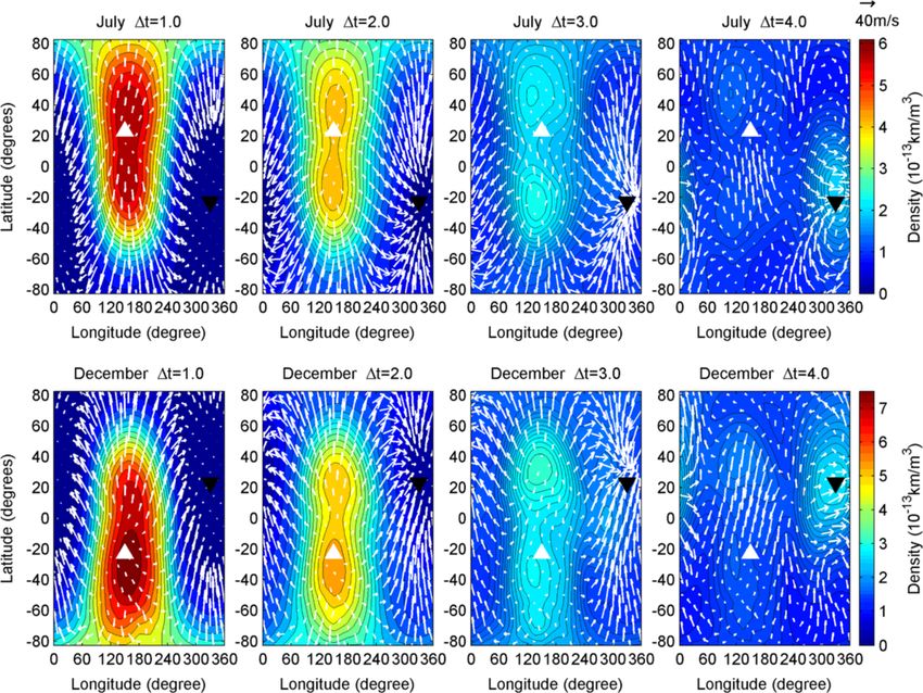
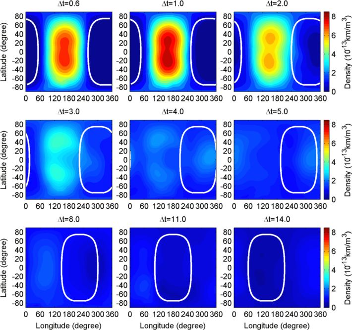
Le et al. Earth, Planets and Space (2015) 67:3                                                                                       Page 2 of 14

 Figure 1 Solar EUV relative variation as a function of wavelength bin and time after flare onset. The relative variation refers to the ratio of
 solar EUV flux after solar flare to that before the solar flare. The wavelength bins of 1 to 37 correspond to wavelength 0 to 105 nm.

 Figure 2 Simulated global variations in neutral density at 400 km at different times after the solar flare. The solid lines in each panel
 indicate the solar terminator at an altitude of 200 km.
Le et al. Earth, Planets and Space (2015) 67:3                                                                                      Page 3 of 14

the thermospheric density at 400 km can increase by as                    average enhancement of 10% ~ 13% in neutral density at
much as 14.6% in about 2 h and takes 12 h to return                       the altitude of 400 km at mid-low latitudes within about
back to a normal state. Qian et al. (2010) also in-                       4 h after solar flare onset. In this study, we would explore
vestigated the ionosphere and the thermosphere re-                        the global thermospheric disturbances induced by a solar
sponse to the X17 solar flare on 28 October 2003 by the                   flare with magnitude of X5 and the transport process of
thermosphere-ionosphere-mesosphere electrodynamics                        energy by using the Global Coupled Ionosphere-
general circulation model (TIME-GCM). The results                         Thermosphere-Electrodynamics Model, developed by the
also show the significant thermospheric disturbances in-                  Institute of Geology and Geophysics, Chinese Academy of
cluding about a maximum increase of 20% in neutral                        Sciences (GCITEM).
density at altitude of 400 km.
   As mentioned above, there are many studies focusing                    Methods
on ionospheric and thermospheric responses to the great                   GCITEM model introduction
X17 solar flare on 28 October 2003. How about a weaker                    The model employed in this study is the GCITEM model
flare’s effect on the thermosphere? Le et al. (2012) sta-                 (Ren et al. 2009). It is a new global 3-D self-consistent
tistically analyzed the neutral density variation for all                 model of the ionosphere and thermosphere including
X-class solar flares during 2001 to 2006 based on the                     electrodynamics. This new model self-consistently calcu-
density data derived from accelerometers on the CHAMP                     lates the time-dependent 3-D structures of the main ther-
and GRACE satellites. The observed results show the                       mospheric and ionospheric parameters in the height range
density response for X1 to X5 flares falls within the noise               from 90 to 600 km, including neutral number density of
level in the thermosphere, but there is significant neutral               the major species O2, N2, and O and the minor species
density response for X5 and stronger flares, with an                      N(2D), N(4S), NO, He, and Ar; ion number densities of

 Figure 3 Percentage variations in neutral density at 400 km at different times after the solar flare. The solid lines in each panel indicate
 solar terminator at an altitude of 200 km.
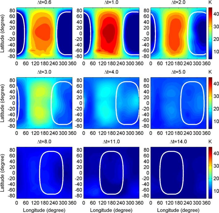
Le et al. Earth, Planets and Space (2015) 67:3                                                                                    Page 4 of 14

O+, O2+, N2+, NO+, N+, and electron; neutral, electron,                  Thus, it is an effective platform to simulate solar flare ef-
and ion temperature; and neutral wind vectors. The iono-                 fects on the thermosphere and ionosphere. In this study,
spheric electric fields in the mid and low latitudes can also            we focus on the thermospheric responses to a solar flare.
be self-consistently calculated. The model is based on the
hydrostatic assumption. It is a full 3-D code with 5° lati-              Simulations
tude by 7.5° longitude grids in a spherical geomagnetic co-              In this study, we modeled the thermospheric responses
ordinate system. The vertical grid spacing is about 3 km                 to an X5 solar flare. The solar EUV variation during an
in the lower thermosphere and about 30 km in the upper                   about X5 solar flare on 6 April 2001 is used in the simu-
thermosphere. This model is solved by a time-stepping                    lations. The EUV variation during the solar flare is cal-
finite difference procedure, with a time step of 2 ~ 5 min.              culated by the Flare Irradiance Spectral Model (FISM).
The horizontal difference procedure uses explicit nu-                    The ratio of EUV flux during the flare to that before the
merical method. To get the rapid vertical molecular dif-                 flare (EUVflare/EUVpre-flare) as a function of UT time and
fusion, the vertical difference procedure uses implicit                  wavelength is shown in Figure 1. The FISM model is an
numerical method. The GCITEM model can simulate                          empirical model that estimates the solar irradiance at
the ionosphere-thermosphere system in a realistic geo-                   wavelengths from 0.1 to 190 nm at 1-nm resolution. The
magnetic field. This is important in the research of the                 long wavelength channel on the GOES X-ray sensor
couple between the neutrals and ions, and the anomaly of                 (XRS) provides a value of the 0.1 to 0.8 nm irradiance.
the ionospheric and thermospheric spatial-temporal va-                   The GOES XRS values are currently the only near real-
riations. GCITEM-IGGCAS can simulate the complex                         time data that are given on-time scales short enough to
chemistry, thermodynamics, dynamics, and electrodyna-                    represent various changes in irradiance due to solar
mics of the coupled ionosphere-thermosphere system.                      flares; the GOES 0.1 to 0.8 nm fluxes are used as the

 Figure 4 Simulated global variations in neutral temperature at 400 km at different times after the solar flare. The solid lines in each
 panel indicate solar terminator at an altitude of 200 km.
Le et al. Earth, Planets and Space (2015) 67:3 Page 5 of 14
short-term solar flare proxy for FISM. The model has a increase occurs at the subsolar point. The neutral dens-
high temporal resolution of 60 s to model EUV variations ity enhancement is larger at the region with smaller solar
due to solar flares (for details please see Chamberlin et al. zenith angle, which shows the significant effect of solar
2007, 2008). zenith angle on the thermospheric response to a solar
The reference simulation is carried out on 6 April (day flare. The results also show that the thermospheric dens-
of year = 96) with the median solar activity condition ity disturbances mainly focus on the sunlight region at
(F10.7 = 140.0). Then the solar EUV variation during the the initial stage (Δt < 1 h); then the disturbance region
solar flare is embedded in the GCITEM model to model gradually extends to the nightside with time. The results
the thermospheric responses to the solar flare. The time also show that the peak enhancement gradually moves
step in the simulations is 2 min. The solar flare onset is from low latitudes to higher latitudes. For example, the
set at 0100 UT. The differences of neutral density, neu- peak enhancement in the northern hemisphere moves
tral temperature, and horizontal wind between the two from 20° N at Δt = 0.6 h to 40° N at Δt = 3 h. To better
simulations are calculated to represent the responses of show the change of neutral density in both the dayside
density, temperature, and wind. and the nightside, the percentage changes (ΔNn) at
different times are plotted in Figure 3. We can find sig-
Results and discussion nificant increases in the dayside with a peak of appro-
The absolute change of neutral density between the flare ximately 15% at the subsolar point. We also can find
simulation and the reference simulation is calculated. Δt significant disturbances in the nightside and later at
is the time after the solar flare onset. The absolute Δt = 2. The peak enhancement at the antisolar point
change of neutral density at 400 km at different Δt from reaches as large as 12%, just a little smaller than that at
0.6 to 14 h is illustrated in Figure 2. The results show the subsolar point.
significant increases in the whole dayside hemisphere Figure 4 illustrates the change of neutral temperature
including high latitudes and polar region. The largest (ΔTn) at 400 km between the flare simulation and the
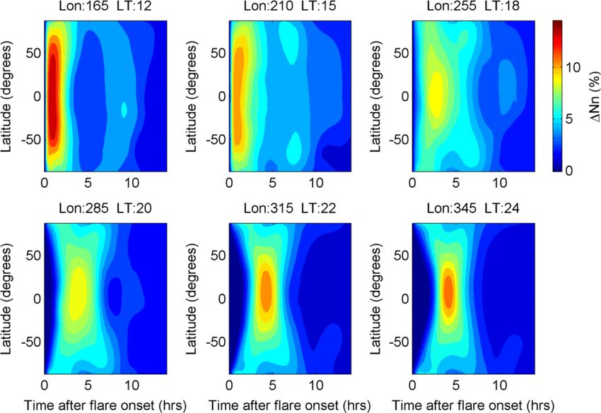
Figure 5 Temporal evolution of the percentage variation of neutral density at 400 km along various meridian planes.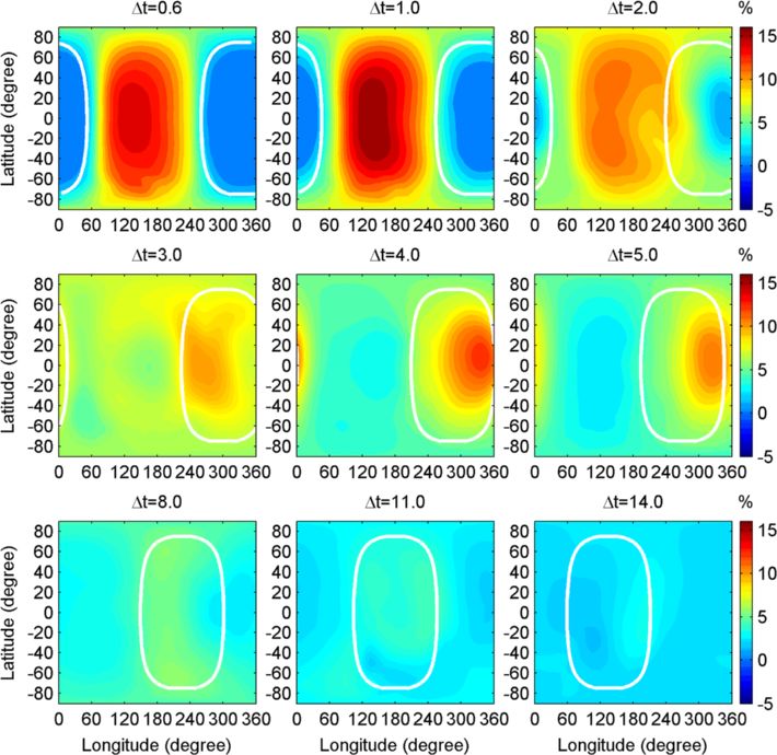
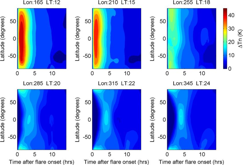
Le et al. Earth, Planets and Space (2015) 67:3                                                                             Page 6 of 14

reference simulation. The results show that the change              time is at 2400 LT. The results show that the thermo-
in neutral temperature has similar variations with that of          spheric density responses to the solar flare are synchro-
the neutral density. There is a peak increase of about              nous for all latitudes in the dayside because all latitudes
45 K in the dayside and about 19 K in the nightside. In             are in the sunlight region. For dayside region like the
the thermosphere, the primary source of the energy go-              meridian planes 165° E (12 LT) and 210° E (15 LT), the
ing to the neutrals is solar EUV radiation; at the higher           peak enhancement occurs at about 0.9 h after the flare
latitudes, the Joule heating becomes dominant at times.             onset. However, for the dusk region (18 LT), the peak
During a solar flare, the enhanced solar EUV radiation              enhancement occurs later, at approximately 2.5 h after
causes the additional heating of the thermosphere gas               the flare onset. As for the nightside, the density distur-
(Schunk and Nagy 2000), which results in increase in                bance is not synchronous for different latitudes. The
neutral temperature. The increase in neutral tempe-                 polar region and high latitudes respond to the solar flare
rature would then alter the scale height of the neutral             earliest because the altitude of 200 km and above is still
height, which causes increase in the neutral density at a           in the sunlight. For other latitudes, the disturbance ap-
fixed height like 400 km as shown in Figure 2; that is,             pears later at the lower latitudes. The temporal evolution
heating below a specific altitude causes the density en-            of the changes of neutral temperature at 400 km along
hancement at the altitude and above.                                various meridian planes from dayside to nightside is
   The temporal evolution of the percentage changes of              illustrated in Figure 6. As mentioned above, the density
neutral density at 400 km along various meridian planes             increases are mainly due to the increase in neutral
from dayside to nightside is illustrated in Figure 5. The           temperature. Thus, we can find similar variations in
solar flare onset is set at 0100 UT. So the subsolar point          neutral temperature with the neutral density variations.
when the flare erupts is in the meridian plane 165° E               For the dayside, the peak enhancement of neutral tem-
where the time is at 1200 LT. the corresponding antiso-             perature occurs around the subsolar point at about 0.9 h
lar point lies in the meridian plane 345° E where the               after the flare onset. For the nightside, the peak

 Figure 6 Temporal evolution of the percentage variation of neutral temperature at 400 km along various meridian planes.
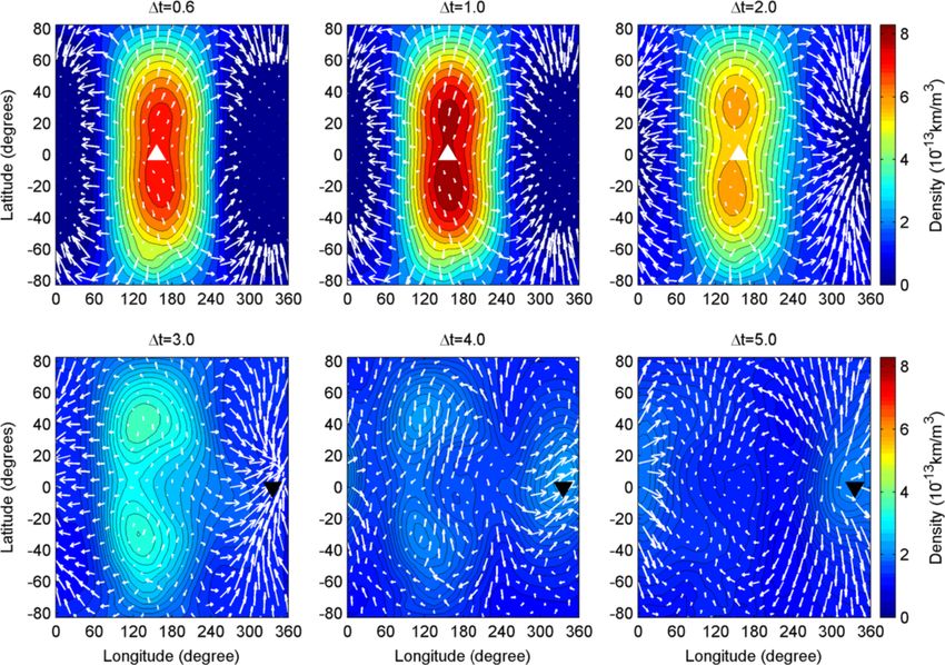
Le et al. Earth, Planets and Space (2015) 67:3                                                                                Page 7 of 14

enhancement of neutral temperature occurs around the                   the solar flare heating disturb the global thermospheric
antisolar point at about 4.0 h after the flare onset.                  atmosphere, which is also an important factor for the day-
   As mentioned above, there are significant disturbances              side and the nightside disturbances in the neutral density.
induced by the solar flare in both the dayside and the                 In the following, we further show the global disturbances
nightside. Figure 7 illustrates the temporal variation of              in the neutral wind and density.
thermospheric average disturbances in the dayside and in                  The absolute change of horizontal wind between the
the nightside. Here we define the dayside as being solar               flare simulation and the reference simulation is also calcu-
zenith angles less than 30°, while the nightside is defined            lated. The variations in horizontal wind at an altitude of
as solar zenith angles larger than 150°. The results show              400 km at different times after the solar flare onset are il-
that after reaching the peak at Δt ≈ 0.9 h, the disturbances           lustrated in Figure 8. The corresponding change in neutral
in the dayside do not decay gradually with time but ap-                density is also plotted the figure. To better understand the
pears as a second peak at Δt ≈ 8 h. The nightside distur-              thermospheric behaviors, the background thermospheric
bances also show a second peak at Δt ≈ 12.5 h after the                density and horizontal wind are plotted in Figure 9. The
first peak at Δt ≈ 4 h. In addition, Figure 7 shows that               neutral density has two peaks at latitudes of about ±25°,
there is the similar but weaker perturbation in the vari-              which is known as equatorial mass anomaly (EMA). The
ation of neutral temperature compared to that of neutral               background horizontal wind at the altitude of 400 km has
density. The solar flare may excite atmospheric waves,                 the maximum value of about 300 m/s. The results show
which transports the disturbed energy in the dayside to                the significant change in global horizontal wind. In the ini-
the nightside and then disturbs the thermospheric atmos-               tial stage of solar flare (Δt = 0.6 h), we can find the evident
phere in the nightside. The global wind changes caused by              change of horizontal wind in the dayside with the

 Figure 7 Temporal evolution of dayside average and nightside average responses to the solar flare. Neutral density (a) and neutral
 temperature (b).
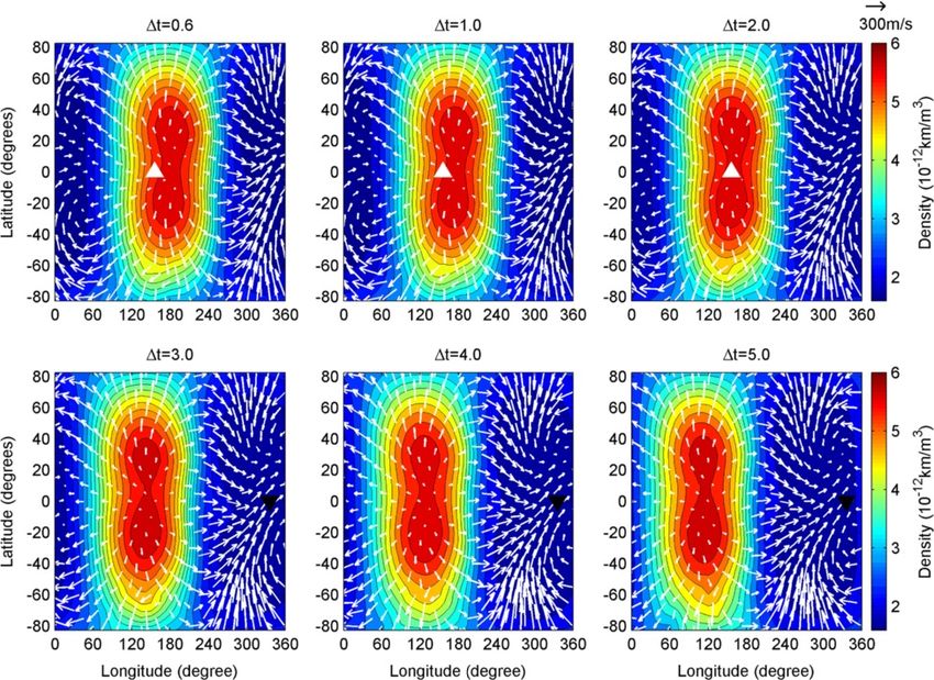
Le et al. Earth, Planets and Space (2015) 67:3                                                                                              Page 8 of 14

 Figure 8 Variation in horizontal wind at an altitude of 400 km at different times after solar flare onset. The corresponding change in
 neutral density also is plotted. The white triangle indicates the subsolar point when the solar flare erupts. The black inverted triangle indicates the
 antisolar point when the solar flare erupts.

minimum at the subsolar point and the maximum around                            The simulations were carried out around March equi-
the solar terminator. The enhanced solar EUV flux heats                       nox. The subsolar point locates around the equator, so
the thermosphere gas and then the thermosphere expands                        the simulated results show a symmetric thermospheric
from low altitudes to higher altitudes and from dayside to                    disturbance in the southern and northern hemispheres.
nightside. As shown in Figure 8, the place of peak en-                        If the solar flare occurs in other seasons, we can find
hancement moves from the subsolar point to higher lati-                       the seasonal difference in the thermospheric responses.
tudes, which is driven by the horizontal wind. The                            Figure 10 illustrates the simulated results in July sol-
gradient of heating rate is largest in the solar terminator                   stice and in December solstice. The results also show
line. Thus, the change of the horizontal wind can be found                    significant enhancements in neutral density in the
to be largest in the solar terminator. As shown in Figure 9,                  dayside with a peak at subsolar point, as well as en-
there is significant neutral wind from dayside to nightside                   hancements in the nightside with a peak at antisolar
due to the heating pressure from the solar radiation                          point. For July solstice, the significant disturbances in
heating in the dayside. The enhanced solar radiation                          the nightside occur in the southern hemisphere. For
strengthens such a global circulation. Therefore, we can                      December, the significant disturbances in the nightside
see from Figures 8 and 9 that both the background neutral                     occur in the northern hemisphere. We can also find the
wind and the change in neutral wind have significant con-                     significant disturbances in thermospheric global circu-
vergence process from high latitudes to low latitudes and                     lation both in July solstice and in December solstice.
from dayside to nightside. The global thermospheric cir-                      There is a significant convergence to the antisolar point
culation causes the significant variation in the nightside                    around Δt = 3 h for both July solstice and December
and also affects the variation in the dayside.                                solstice.
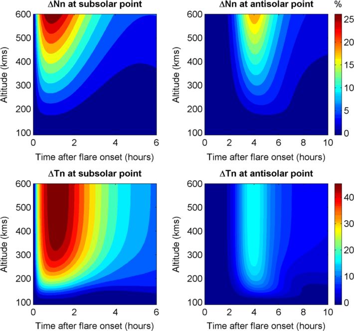
Le et al. Earth, Planets and Space (2015) 67:3                                                                                 Page 9 of 14

 Figure 9 Same as Figure 8, but for the background horizontal wind and neutral density. The white triangle indicates the subsolar point
 when the solar flare erupts.

   The height dependence of the thermospheric res-                     of electron and ions. The time and amplitude of the
ponses to a solar flare is shown in Figure 11. Left panels             peak response are determined by peak solar irradiance
illustrate the neutral density and neutral temperature re-             (e.g., Afraimovich 2000; Zhang et al. 2002, 2011; Le et al.
sponses at the subsolar point. Right panels illustrate the             2007). However, because of the large mass and high heat
corresponding response at the antisolar point. The re-                 capacity in the thermosphere, the neutral gas response
sults show that the percentage enhancement in neutral                  to a solar flare would be sluggish with regard to transi-
density increases with altitude for both the subsolar                  ent enhancement in solar EUV flux; that is, it needs lon-
point in the dayside and the antisolar point in the night-             ger time for neutral gas to react to the increase in solar
side. There is a very small change of neutral density                  EUV flux, and the neutral gas response also can last a
below 150 km. The neutral density responses to the                     longer time. Our simulations just show such a feature.
solar flare reach the peak almost at the same time (Δt ≈               For example, the percentage change of neutral density at
0.9 h) for all altitudes. The results show that the en-                subsolar point reaches the peak at Δt ≈ 1 h when the
hancement in neutral temperature increases with alti-                  EUV flux return to the normal level, and it takes as long
tude for the altitude range from 100 to 350 km, but it                 as more than 20 h to return back to the background
has almost the same magnitude at altitudes of 350 km                   level.
above. The height distribution of the increase in neutral                Based on the analyses of the thermospheric response
temperature is similar with the temperature structure of               to all X-class solar flares during 2001 to 2006, Le et al.
the thermosphere.                                                      (2012) found that the thermospheric density enhance-
   It is well known that the ionospheric response to a                 ment is much more correlated with integrated EUV
solar flare is very fast because of the small time constant            flux than with peak EUV flux, which suggests that the
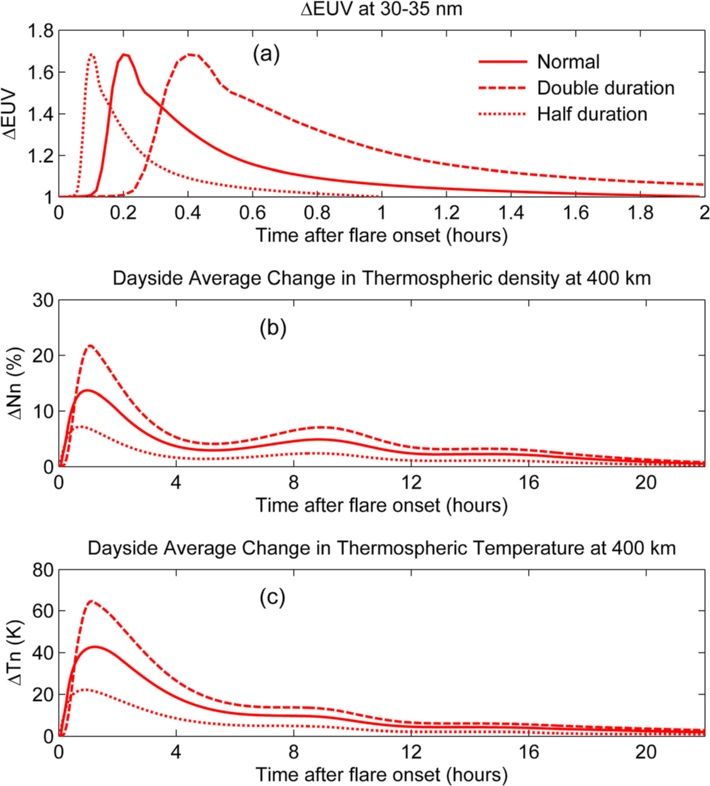
Le et al. Earth, Planets and Space (2015) 67:3                                                                                          Page 10 of 14

 Figure 10 Seasonal difference of thermospheric responses to a solar flare. Upper panels for July solstice and lower panels for December
 solstice. The arrow indicates the change of horizontal wind. The color indicates the change of neutral density. The white triangle indicates the
 subsolar point when the solar flare erupts. The black inverted triangle indicates the antisolar point when the solar flare erupts.

thermospheric response is strongly dependent on the                          energy compared to the normal condition and the sec-
total integrated energy into the thermosphere. Based on                      ond one has the double integrated energy.
the simulations by the GITM, Pawlowski and Ridley                               Figure 12b, c shows the dayside average responses of
(2011) also reported the same feature that the density re-                   neutral density and neutral temperature to the three
sponse at 400 km altitude is dependent on the total inte-                    solar flares: half duration, normal duration, and double
grated energy. To further verify the idea, we carried out                    duration. The peak enhancement in the neutral density
other two simulations with the same peak solar EUV                           is 21.7%, 13.7%, and 7.1% for the double duration flare,
flux but different duration of EUV enhancement. For the                      the normal flare, and the half duration flare, respectively.
first simulation, the solar flare duration is shortened by a                 The peak increase in neutral temperature is 64.5, 42.8,
half with the peak value unchanged. For the second one,                      and 22.2 K for the double duration flare, the normal
the solar flare duration is lengthened by 100% with the                      flare, and the half duration flare, respectively. The results
peak value unchanged. Take the relative change of EUV                        suggest that although with the same peak EUV flux,
(ΔEUV) at 30 to 35 nm during the solar flares as an                          the larger integrated energy being deposited into the at-
example. The ΔEUV is the ratio of the EUV during solar                       mosphere results in the larger thermospheric responses.
flare to the EUV before solar flare. The temporal of                         Pawlowski and Ridley (2011) reported a linear depen-
ΔEUV during the three solar flares (normal duration,                         dence of neutral density response on the total integrated
double duration, and half duration) is illustrated in                        energy. Our simulations show that is not a rigorous
Figure 12a; that is, the first one has half integrated                       linear dependence between the density response and the
Le et al. Earth, Planets and Space (2015) 67:3                                                                                  Page 11 of 14

 Figure 11 Height variation of neutral density and neutral temperature responses to a solar flare. Left panels for the subsolar point and
 right panels for the antisolar point.

total integrated energy. The peak enhancement in the                    the CHAMP before and after the 6 April 2001 X5.6 solar
neutral density does not increase by 100% but only in-                  flare is calculated. With a near-polar inclination, the sat-
crease by approximately 58% when the flare duration                     ellite provides near-global coverage at an approximate
prolongs by 100% from the normal condition to double                    altitude of 410 km within two local time sectors at most
duration. These results show that the enhancement in                    latitudes. All density data has been averaged into 3° lati-
neutral density increases nonlinearly with integral EUV                 tudinal bins to reduce any random errors. In addition,
flux. Its amplification decreases with integral EUV flux.               neutral density has also been normalized to a fixed
  Figure 12 (normal duration lines) also illustrates the                height of 400 km using the NRL-MSISe-00 empirical
dayside average disturbance level of thermospheric density              density model. Figure 13 illustrates the temporal vari-
and temperature at 400 km. The results show that there is               ation in the dayside sector (14.4 LT) and in the nightside
a peak enhancement of about 13.7% in the global average                 sector (2.4 LT). The observed results show significant
neutral density at 400 km and a peak increase of about                  density increases in the dayside after the flare. The
42 K in the global average neutral temperature at 400 km.               nightside observations also show some enhancements
It takes about 20 h for the density enhancement to drop                 several hours after the flare. Figure 13 also shows that
to 1% and takes about 20 h for the temperature increase                 the enhancements in the dayside mainly appear in the
to drop to 2 K. These results show that the thermospheric               middle-low latitudes. As for the nightside, the enhance-
responses to a solar flare can last more than 20 h, which is            ments first appear in the high latitudes and then extend
much longer than the ionospheric responses of which the                 gradually to the middle and low latitudes. These tem-
typical duration is less than 2 h (Tsurutani 2005; Le et al.            poral and spatial features are basically in agreement with
2007).                                                                  the simulations mentioned above.
  To verify the simulated result of this study, the ther-                  To further quantitatively compare the observations
mospheric density derived from the accelerometers on                    and the simulations, the latitude distributions of the
Le et al. Earth, Planets and Space (2015) 67:3                                                                                           Page 12 of 14

 Figure 12 The relative change of EUV and dayside average change in the thermosphere. (a) The relative change of EUV at 30 to 35 nm
 during the solar flare. The solid line, the dashed line, and the dotted line refer to the EUV variation with normal duration, double duration, and
 dotted duration, respectively. Dayside average change in thermospheric density (b) and temperature (c) at 400 km.

enhancements are calculated and shown in Figure 14.                           simulations and observations suggests that the GCITEM
The mean of three orbits before the flare onset is calcu-                     model can well model the thermospheric responses to a
lated as the reference value. Thus, we can get the re-                        solar flare.
ference value at each latitude bin. To investigate the
neutral density responses to solar flares in the dayside,                     Conclusions
the responses of the first three orbits (corresponding to                     The thermospheric responses to a solar flare were inves-
the time within about 4 h) after solar flare onset are cal-                   tigated, based on the results of a modeling effort by the
culated and their mean percentage change is taken as                          GCITEM model. The solar EUV variation during a solar
the response for the solar flare. As for the nightside, the                   flare is derived from the empirical model FISM. In this
mean percentage change within 8 h after the solar flare                       study, we did not model the thermospheric response to
onset is calculated. The corresponding simulated results                      the great solar flare like the X17 solar flare on 28 October
are also calculated. Both the observed results and simu-                      2003, but modeled the effects of a weaker flare of X5. The
lated results are plotted in Figure 14. We can find that                      simulated results show that there are significant enhance-
the simulated results are basically consistent with the                       ments in the neutral density and neutral temperature.
observed results, although the observed results have lar-                     The strongest responses of the thermosphere occur at
ger latitudinal fluctuation. The comparison between the                       the subsolar point. The larger solar zenith angle causes
Le et al. Earth, Planets and Space (2015) 67:3                                                                                           Page 13 of 14

 Figure 13 Latitude versus time depictions of total mass density. Latitude versus time depictions of total mass density in dayside (left panel)
 and nightside (right panel) measured by CHAMP satellite during the 6 April 2001 X5.6 solar flare. The density is normalized to 400 km.

the smaller thermospheric responses, which suggests the                      latitudes. The peak disturbance in the nightside appears
strong effect of the solar zenith angle. The peak responses                  at the antisolar point. The heating from the sudden
appear about 1 h after the solar flare onset for all latitudes.              increases in solar radiation during a solar flare disturbs
The thermospheric responses to a solar flare can last more                   the global thermosphere circulation, which results in the
than 20 h.                                                                   significant change in the horizontal wind. There is sig-
   In addition to the significant disturbances in the day-                   nificant convergence process to the antisolar point, and
side, the simulated results also show that a solar flare                     thus the strong disturbances in the nightside occur at
can produce significant disturbance in the nightside. The                    the antisolar point. The peak enhancement in the night-
percentage change of the neutral density in the nightside                    side appears about 4 h after the solar flare onset. In
is just a little smaller than that in the dayside. There is a                addition, our simulations show that although with the
significant latitude dependence for nightside thermo-                        same peak EUV flux, the solar flare with longer duration
spheric response. It almost synchronizes with dayside in                     would produce the stronger thermospheric response,
the polar region and high latitudes but is later at lower                    which suggests that the integral energy during a solar

 Figure 14 Latitudinal distribution of average change of neutral density at 400 km. Left panel for dayside and right panel for nightside.
 Circle lines for the observations from CHAMP and solid lines for the simulations. For details of calculations of the percentage change, see the text.
Le et al. Earth, Planets and Space (2015) 67:3                                                                                                          Page 14 of 14

flare is an important factor of the thermospheric                                     Mahajan KK, Lodhi NK, Upadhayaya AK (2010) Observations of X-ray and EUV
responses to a solar flare. To verify quantitatively the re-                              fluxes during X-class solar flares and response of upper ionosphere.
                                                                                          J Geophys Res 115:A12330. doi:10.1029/2010JA015576
sult of this modeling study, the simulated results are                                Pawlowski DJ, Ridley AJ (2008) Modeling the thermospheric response to solar
compared with the observations of neutral density de-                                     flares. J Geophys Res 113:A10309. doi:10.1029/2008JA013182
rived from the accelerometers on the CHAMP satellite.                                 Pawlowski DJ, Ridley AJ (2009) Modeling the ionospheric response to the 28
                                                                                          October 2003 solar flare due to coupling with the thermosphere. Radio Sci
The simulated results are basically consistent with the                                   44:RS0A23. doi:10.1029/2008RS004081
observed results, although the observed results have lar-                             Pawlowski DJ, Ridley AJ (2011) The effects of different solar flare characteristics
ger latitudinal fluctuation.                                                              on the global thermosphere. J Atmos Terr Phys 73:1840–1848.
                                                                                          doi:10.1016/j.jastp.2011.04.004
                                                                                      Qian L, Burns AG, Chamberlin PC, Solomon SC (2010) Flare location on the solar
Competing interests                                                                       disk: modeling the thermosphere and ionosphere response. J Geophys Res
The authors declare that they have no competing interests.                                115:A09311. doi:10.1029/2009JA015225
                                                                                      Ren Z, Wan W, Liu L (2009) GCITEM-IGGCAS: a new global coupled ionosphere-
                                                                                          thermosphere-electrodynamics model. J Atmos Sol Terr Phys 71
Authors’ contributions
                                                                                          (17&18):2064–2076
HL planned and led the study, interpreted the results, and drafted the
                                                                                      Schunk RW, Nagy AF (2000) Ionospheres: physics, plasma physics, and chemistry.
manuscript. ZR constructed the model for the simulations. YC, LL, and HZ
                                                                                          Cambridge Atmos Space Sci Ser 59
participated in the data analysis and interpretation. All authors read and
                                                                                      Sutton EK, Forbes JM, Nerem RS, Woods TN (2006) Neutral density response to
approved the final manuscript.
                                                                                          the solar flares of October and November, 2003. Geophys Res Lett 33:L22101.
                                                                                          doi:10.1029/2006GL027737
Acknowledgements                                                                      Tsurutani BT (2005) The October 28, 2003 extreme EUV solar flare and resultant
This research was supported by the Chinese Academy of Sciences project                    extreme ionospheric effects: comparison to other Halloween events and the
(KZZD-EW-01-3), National Key Basic Research Program of China                              Bastille Day event. Geophys Res Lett 32:L03S09. doi:10.1029/2004GL021475
(2012CB825604), National Natural Science Foundation of China (41374162,               Wan W, Liu L, Yuan H, Ning B, Zhang S (2005) The GPS measured SITEC caused
41231065, and 41321003).                                                                  by the very intense solar flare on July 14, 2000. Adv Space Res 36:2465–2469.
                                                                                          doi:10.1016/j.asr.2004.01.027
Received: 5 September 2014 Accepted: 1 December 2014                                  Zhang DH, Xiao Z (2005) Study of ionospheric response to the 4B flare on 28
                                                                                          October 2003 using international GPS service network data. J Geophys Res
                                                                                          110:A03307. doi:10.1029/2004JA010738
                                                                                      Zhang DH, Xiao Z, Chang Q (2002) The correlation of flare's location on solar disc
References                                                                                and the sudden increase of total electron content. Chin Sci Bull 47(1):82–85
Afraimovich EL (2000) GPS global detection of the ionospheric response to solar       Zhang DH, Mo XH, Cai L, Zhang W, Feng M, Hao YQ, Xiao Z (2011) Impact factor
     flares. Radio Sci 35(6):1417–1424. doi:10.1029/2000RS002340                          for the ionospheric TEC response to solar flare irradiation. J Geophys Res
Chamberlin PC, Woods TN, Eparvier FG (2007) Flare Irradiance Spectral Model               116:A04311. doi:10.1029/2010JA016089
     (FISM): daily component algorithms and results. Space Weather 5:S07005.
     doi:10.1029/2007SW000316
Chamberlin PC, Woods TN, Eparvier FG (2008) Flare Irradiance Spectral Model
     (FISM): flare component algorithms and results. Space Weather 6:S05001.
     doi:10.1029/2007SW000372
Forbes JM, Lu G, Bruinsma S, Nerem S, Zhang X (2005) Thermosphere density
     variations due to the 15–24 April 2002 solar events from CHAMP/STAR
     accelerometer measurements. J Geophys Res 110:A12S27.
     doi:10.1029/2004JA010856
Le H, Liu L, Chen B, Lei J, Yue X, Wan W (2007) Modeling the responses of the
     middle latitude ionosphere to solar flares. J Atmos Solar Terr Phys
     69:1587–1598. doi:10.1016/j.jastp.2007.06.005
Le H, Liu L, He H, Wan W (2011) Statistical analysis of solar EUV and X-ray flux
     enhancements induced by solar flares and its implication to upper
     atmosphere. J Geophys Res 116, A11301. doi:10.1029/2011JA016704
Le H, Liu L, Wan W (2012) An analysis of thermospheric density response
     to solar flares during 2001–2006. J Geophys Res 117:A03307.
     doi:10.1029/2011JA017214
Le H, Liu L, Chen Y, Wan W (2013) Statistical analysis of ionospheric responses to
     solar flares in the solar cycle 23. J Geophys Res Space Physics 118:576–582.
     doi:10.1029/2012JA017934
Leonovich LA, Afraimovich EL, Romanova EB, Taschilin AV (2002) Estimating the
     contribution from different ionospheric regions to the TEC response to the            Submit your manuscript to a
     solar flares using data from the international GPS network. Ann Geophys
     20:1935–1941. doi:10.5194/angeo-20-1935-2002                                          journal and benefit from:
Liu JY, Lin CH, Tsai HF, Liou YA (2004) Ionospheric solar flare effects monitored
     by the ground-based GPS receivers: theory and observation. J Geophys Res              7 Convenient online submission
     109:A01307. doi:10.1029/2003JA009931                                                  7 Rigorous peer review
Liu JY, Lin CH, Chen YI, Lin YC, Fang TW, Chen CH, Chen YC, Hwang JJ (2006)                7 Immediate publication on acceptance
     Solar flare signatures of the ionospheric GPS total electron content.                 7 Open access: articles freely available online
     J Geophys Res 111:A05308. doi:10.1029/2005JA011306
                                                                                           7 High visibility within the field
Liu H, Lühr H, Watanabe S, Ko¨hler W, Manoj C (2007) Contrasting behavior of
     the thermosphere and ionosphere in response to the 28 October 2003 solar              7 Retaining the copyright to your article
     flare. J Geophys Res 112:A07305. doi:10.1029/2007JA012313
Liu L, Wan W, Chen Y, Le H (2011) Solar activity effects of the ionosphere: a brief
                                                                                              Submit your next manuscript at 7 springeropen.com
     review. Chin Sci Bull 56(12):1202–1211. doi:10.1007/s11434-010-4226-9
You can also read