GO WITH THE FLOW: ADAPTIVE CONTROL FOR NEURAL ODES
←
→
Page content transcription
If your browser does not render page correctly, please read the page content below
Preprint. Under review

                                        G O WITH THE FLOW:
                                        A DAPTIVE C ONTROL FOR N EURAL ODE S
                                         Mathieu Chalvidal1,2,3 , Matthew Ricci2 , Rufin VanRullen1,3 , Thomas Serre1,2
                                         1
                                           Artificial and Natural Intelligence Toulouse Institute, Universite de Toulouse, France
                                         2
                                           Carney Institute for Brain Science, Dpt. of Cognitive Linguistic & Psychological Sciences
                                         Brown University, Providence, RI 02912
                                         3
                                           Centre de Recherche Cerveau & Cognition CNRS, Université de Toulouse
                                         UMR 5549, Toulouse 31055 France
                                         {mathieu chalvid, mgr, thomas serre}@brown.edu
                                         rufin.vanrullen@cnrs.fr
arXiv:2006.09545v2 [cs.LG] 7 Oct 2020

                                                                                     A BSTRACT
                                                 Despite their elegant formulation and lightweight memory cost, neural ordinary
                                                 differential equations (NODEs) suffer from known representational limitations.
                                                 In particular, the single flow learned by NODEs cannot express all homeomor-
                                                 phisms from a given data space to itself, and their static weight parametrization
                                                 restricts the type of functions they can learn compared to discrete architectures
                                                 with layer-dependent weights. Here, we describe a new module called neurally-
                                                 controlled ODE (N-CODE) designed to improve the expressivity of NODEs. The
                                                 parameters of N-CODE modules are dynamic variables governed by a trainable
                                                 map from initial or current activation state, resulting in forms of open-loop and
                                                 closed-loop control, respectively. A single module is sufficient for learning a dis-
                                                 tribution on non-autonomous flows that adaptively drive neural representations.
                                                 We provide theoretical and empirical evidence that N-CODE circumvents limita-
                                                 tions of previous models and show how increased model expressivity manifests
                                                 in several domains. In supervised learning, we demonstrate that our framework
                                                 achieves better performance than NODEs as measured by both training speed and
                                                 testing accuracy. In unsupervised learning, we apply this control perspective to an
                                                 image autoencoder endowed with a latent transformation flow, greatly improving
                                                 representational power over a vanilla model and leading to state-of-the-art image
                                                 reconstruction on CIFAR-10.

                                        1   I NTRODUCTION
                                        The interpretation of artificial neural networks as continuous-time dynamical systems opens has led
                                        to both theoretical and practical advances in representation learning. According to this interpretation,
                                        the separate layers of a deep neural network are understood to be a discretization of a continuous-
                                        time operator so that, in effect, the net is infinitely deep. One important class of continuous-time
                                        models, neural ordinary differential equations (NODEs) (Chen et al., 2018), have found natural ap-
                                        plications in generative variational inference (Grathwohl et al., 2018) and physical modeling (Köhler
                                        et al., 2019; Ruthotto et al., 2020) because of their ability to take advantage of black-box differential
                                        equation solvers and correspondence to dynamical systems in nature.
                                        Nevertheless, NODEs suffer from known representational limitations, which researchers have tried
                                        to alleviate either by lifting the NODE activation space to higher dimensions or by allowing the
                                        transition operator to change in time, making the system non-autonomous (Dupont et al., 2019) .
                                        For example, Zhang et al. (2020) showed that NODEs can arbitrarily approximate maps from Rd to
                                        R if NODE dynamics operate with an additional time dimension in Rd+1 and the system is affixed
                                        with an additional linear layer. The same authors showed that NODEs could approximate homeo-
                                        morphisms from Rd to itself if the dynamics were lifted to R2d . Yet, the set of homeomorphisms
                                        from Rd to itself is in fact quite a conservative function space from the perspective of represen-
                                        tation learning, since these mappings preserve topological invariants of the data space, preventing
                                        them from “disentangling” data classes like those of the annulus data in Fig. 1 (lower left panel).

                                                                                           1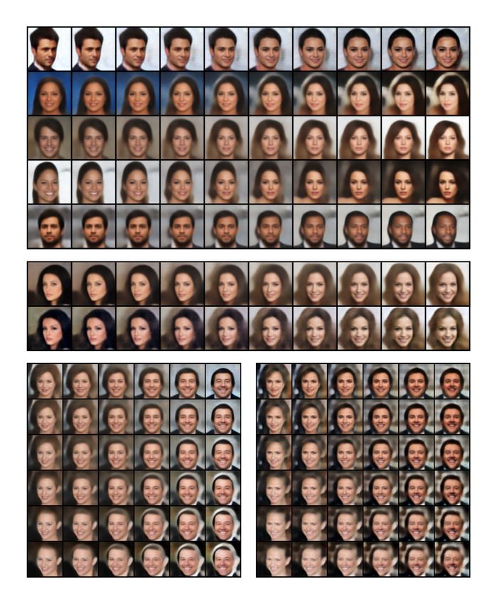
Preprint. Under review

In general, much remains to be understood about the continuous-time framework and its expressive
capabilities.
In this paper, we propose a new approach that we
call neurally-controlled ODEs (N-CODE) designed
to increase the expressivity of continuous-time neu-
ral nets by using tools from control theory. Whereas
previous continuous-time methods learn a single,
time-varying vector field for the whole input space,
our system learns a family of vector fields param-
eterized by data. We do so by mapping the input
space to a collection of control weights which in-
teract with neural activity to optimally steer model
dynamics. These time-varying control weights form
the time-varying parameters of a dynamical system,
making N-CODE akin to a continuous-time hyper-
network (Ha et al., 2016). The implications of this
new formulation are critical for model expressivity.
In particular, the transformation of the input space is
no longer constrained to be a homeomorphism, since
the flows associated with each datum are specifically         Figure 1: Vector fields for continuous-time neu-
adapted to that point. Consequently, our system can           ral networks. Integral curves with arrows show
easily “tear” apart the two annulus classes in Fig. 1         the trajectories of data points under the influence
(lower right panel) without directly lifting the data         of the network. (Top left) Standard NODEs learn a
space to a higher dimension.                                  single time-independent flow (in black) that must
                                                              account for the whole data space. (Top right) N-
The rest of the paper proceeds as follows. First,             CODE learns a family of vector fields (red vs yel-
we will lay out the background for N-CODE and its             low vs blue), enabling the system to flexibly ad-
technical formulation. Then, we will demonstrate its          just the trajectory for every data point. (Bottom
efficacy in two cases, one supervised and one un-             left) Trained NODE trajectories of initial values
supervised. In the supervised case, we show how               in a data set of concentric annuli, colored green
N-CODE can classify data by learning to bifurcate             and yellow. The NODE transformation is a home-
                                                              omorphism on the data space and cannot separate
its dynamics along class boundaries. Then, we show            the classes as a result. Colored points are the ini-
how the flows learned by N-CODE can be used as                tial state of the dynamics, and black points are the
latent representations in an autoencoder, leading to          final state. (Bottom right) Corresponding flows for
state-of-the-art reconstruction on CIFAR10.                   N-CODE which easily separate the classes. Tran-
                                                              siting from the inner to outer annulus effects a bi-
                                                              furcation which linearly separates the data.
2   BACKGROUND
Neural ODEs (NODEs) (Chen et al., 2018) consist of a differentiable nonlinear mapping f : X ×
R × Θ 7→ X parameterized by a vector θ ∈ Θ and defining a continuous vector field over a feature
space X . The corresponding equation of motion
                                               dx
                                                   = f (x, θ, t)                             (1)
                                                dt
gives rise to a flow, i.e a triple (X , R, Φθ ) with Φθ : X × R 7→ X defined by:
                                                          ZT
                              Φθ (x(0), T ) = x(0) +           f (x(t), θ, t)dt                               (2)
                                                          0
which relates an initial point x(0) to an orbit of points {x(t) = Φθ (x(0), t), t ∈ R}. Integrating Φθ
over a specified time horizon results in a homeomorphism of the feature space parametrized by θ.
Several properties of such flows make them appealing for machine learning. For example, the ODEs
that govern such such flows can be solved with off-the shelf solvers and they can potentially model
data irregularly sampled in time. Moreover, such flows are reversible maps by construction whose
inverse is just the system integrated backward in time, Φθ (., t)−1 = Φθ (., −t). This property en-
ables depth-constant memory cost of training thanks to the adjoint sensitivity method (Pontryagin
Lev Semyonovich ; Boltyanskii V G & F, 1962) and the modeling of time-continuous generative
normalizing flows algorithms (Grathwohl et al., 2019).

                                                   2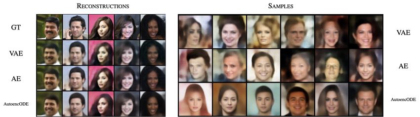
Preprint. Under review
Interestingly, discretizing Eq. 2 coincides with the recursive formulation of a residual network (He
et al., 2015) with a single residual operator fθ :
T
X
ΦResNet (x(0), T ) = x(0) + fθ (xt−1 ) (3)
t=1
In this sense, NODEs with a time-independent (autonomous) transition operator, f , are the infinitely
deep limit of weight-tied residual networks. Relying on the fact that every non-autonomous dy-
namical system with state x ∈ Rd is equivalent to an autonomous system on the extended state
(x, t) ∈ Rd+1 , Eq. 2 can also be used to model general, weight-untied residual networks. However
it remains unclear how dependence of f in time should be modeled in practice and how their dynam-
ics relate to their discrete counterparts with weights evolving freely across blocks through gradient
descent.
3 N-CODE: L EARNING TO CONTROL DATA - DEPENDENT FLOWS
General formulation - The main idea of N-CODE is to consider the parameters, θ, in Eq. 1 as
data-dependent control weights for the dynamical state, x. Model dynamics are then governed by
a coupled system of equations on the extended state z(t) = (x(t), θ(t)). The initial value of the
control weights, θ(0), is given by a mapping γ : X → Θ. Throughout, we assume that the initial
time point is t = 0. The full trajectory of control weights, θ(t), is then output by a controller,
g, given by another differentiable nonlinear mapping g : Θ × R × X 7→ Θ with initial condition
γ(x(0)). Given an initial point, x(0), we can solve the initial value problem (IVP):
dz dx , dθ = (f (x, θ, t), g(θ, x, t))
= h(z, t)
dt = dt dt (4)
z(0) = x(0),
(x(0), θ(0)) = (x(0), γ(x(0)))
where h corresponds to the augmented map
h = (f, g). We may think of g and γ as a
collective controller of the dynamical system
with equation of motion, f . We model g and
γ as neural networks parametrized by µ ∈ Rnµ
and use gradient descent techniques where the
gradient can be computed by solving an ad-
joint problem (Pontryagin Lev Semyonovich ;
Boltyanskii V G & F, 1962) that we describe
in the next section. Our goal here is to use
the meta-parameterization via Θ to create richer
dynamic behavior for a given f than directly
optimizing its weights θ.
Well-posedness - If f and g are continuously
differentiable with respect to x and θ and con-
tinuous with respect to t, then, for all ini- Figure 2: Diagram of a general N-CODE module:
tial conditions (x(0), theta(0)), there exists a Given a initial state x(0), the module consists of an aug-
unique solution z for equation 4 thanks to the mented dynamical system that couples activity state x
Cauchy-Lipschitz theorem. This result leads to and weights θ over time (red arrows). A mapping γ
the existence and uniqueness of the augmented infers initial control weights θ0 defining an initial flow
flow (X ×Θ, R, Φµ ) with Φµ : (X ×Θ)×R 7→ (open-loop control). This flow can potentially evolve in
X × Θ. Moreover, considering the restriction time as θ might be driven by a feedback signal from x
of such a flow on X , we are now endowed (closed-loop, dotted line). This meta-parameterization
with a universal approximator for at least the of f can be trained with gradient descent by solving an
augmented adjoint sensitivity system (blue arrows)
set of homeomorphisms on X given that this re-
striction constitutes a non-autonomous system
(Zhang et al., 2019a). We discuss now how g
and γ affect the evolution of the variable x(t), exhibiting two forms of control.
3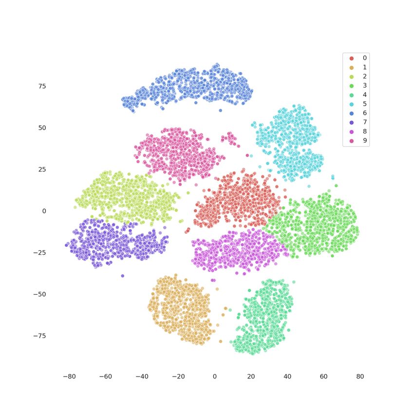
Preprint. Under review
3.1 OPEN AND CLOSED - LOOP CONTROLLERS
If the controller outputs control weights as a function of the current state, x(t), then we say that the
it is a closed-loop controller. Otherwise, it is an open-loop controller.
Open-loop control - First, we consider the effect of using only the mapping γ in equation 4 as a
controller. Here, γ maps the input space X to Θ so that f is conditioned on x(0) but not necessarily
on x(t) for t > 0. In other words, each initial value x(0) evolves according to its own learned flow
(X , R, Φγ(x(0)) ). This allows for particle trajectories to evolve more freely than within a single
flow that must account for the whole data-distribution and resolves the problem of non-intersecting
orbits (see Figure 3). At the distribution level, optimizing γ for a given cost function amounts
to find a push-forward mapping from the distribution on X to the distribution of flows (X , R, Φ)
that minimizes this cost. Note that γ is independent of the way θ parameterizes f . Thus, open-
loop control can be easily combined with recent proposals for modeling equations of motion as
combinations of basis functions, which (Choromanski et al., 2020) used to build non-autonomous
systems.
Closed-loop control - Defining a differentiable mapping g outputting the time-dependent control
weights θ(t) given the state of the variable x(t) yields a non-autonomous system on X . This can
be seen as a specific dimension augmentation technique where additional variables correspond to
the parameters θ. However, contrary to appending extra dimensions which doesn’t change the au-
tonomous property of the system, here this augmentation results in a module describing a time-
varying transformation Φθ(t) (x0 , t). Additionally, the presence of closed-loop feedback might re-
sult in interesting dynamical regimes such as stability, chaos, etc. (Hale, 1969).
4 T RAINING
Loss function - We consider now the following generalized loss function that integrates a cost over
some interval [0, T ]:
ZT ZT
l(z) := `(z(t), t)dt = `(x(t), θ(t), t)dt (5)
0 0
This loss formulation is more general than in (Chen et al., 2018) as one can imagine ` as any
Lebesgue-measurable function. In particular, this encompasses discrete time point penalization or
regularization of activations or weights over the whole trajectory rather than the final state z(T ) of
the system. The following result enables us to compute the gradients of equation 5 with respect to
µ.
Theorem 1 - Augmented adjoint method: Given the IVP of equation 4 and for ` defined in equa-
tion 5, we have
ZT da ∂h ∂`
∂l ∂h = −aT . −
= a(t)T dt, such that a verifies dt ∂z ∂z (6)
∂µ ∂µ a(T ) = O
0 |X |+|Θ|
∂f ∂f
∂h ∂h ∂x ∂θ
where is the Jacobian of h with respect to z: ∂z = .
∂z ∂g ∂g
∂x ∂θ
In practice, we compute the Jacobian for this augmented dynamics with open source automatic
differentiation libraries using Pytorch (Paszke et al., 2019) in order seamlessly integrate N-CODE
modules in bigger architectures. We show an example of such modules in the appendix.
5 E XPERIMENTS
5.1 T OY PROBLEMS
Reflection - We introduce our approach with the 1-dimensional problem posed in (Dupont et al.,
2019), consisting of learning the reflection map ϕ(x) = −x. It has been shown that the vanilla
4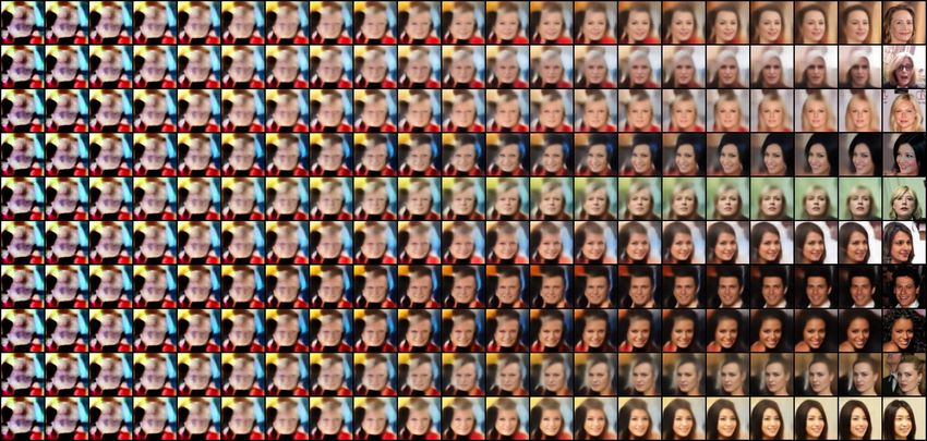
Preprint. Under review

Figure 3: Trajectories over time for three types of continuous-time neural networks learning the 1-dimensional
reflection map ϕ(x) = −x. Left: (NODE) Irrespective of the form of f , a NODE module cannot learn such
a function as trajectories cannot intersect (Dupont et al., 2019). Middle: (Open-loop N-CODE). The model
is able to learn a family of vector fields by controlling a single parameter of f conditioned on x(0). Right:
(Closed-loop N-CODE) With a fixed initialization, x(0), the controller model still learns a deformation of the
vector field to learn ϕ. Note that the vector field is time-varying, contrary to the two others versions.

Figure 4: The concentric annuli problem. A classifier must separate two classes in R2 , a central disk and an
annulus that encircles it. Left: Soft decision boundaries (blue to white) for NODE (First), N-CODE open-loop
((Second) and closed-loop (First) models. Right: Training curve for the three models.

NODE module cannot learn such a function. However, both the open and closed loop formulations
of N-CODE easily fit ϕ, as shown in Figure 3. The conditioning on data allows N-CODE to learn
two separate vector fields, circumventing the topological limitation of the single flow learned by
NODEs. We may interpret the classification decision as resulting from a bifurcation in the model
dynamics. In particular, as x goes from −1 to 1, we can observe the vector field given by f (x)
switching from a negative (blue) to a positive (orange) orientation.
Concentric annuli - We also evaluate our proposed models on the concentric annuli dataset pro-
posed in (Lin & Jegelka, 2018; Dupont et al., 2019). Specifically, we define a class of equations
of motion, f , acting on R2 in the form of a two-layer MLP with 16 hidden units. We train the
models such that the final representations x(T ) must linearly separate the classes on the concentric
classes dataset. We qualitatively evaluated the learned flows’ complexity and their generalization
capabilities by inspecting decision boundaries in Fig. 4. As previously discussed, NODE transfor-
mations are homeomorphisms and preserve the topology of the space, notably the linking number
of data manifolds, which might lead to unstable and complex flows for entangled data manifolds.
In comparison, our proposed method is not affected by this problem, as every trajectory belongs to
its own specific flow, thus breaking the topological constraint of these transformations and allowing
for simpler paths that ease model convergence (see Fig 4). Again, we may think of the classification
decisions as being mediated by a bifurcation parametrized by the data space. Transiting across the
true classification boundary switches the vector field from one pushing points to one side of the
classification boundary to the other. Moreover, the construction of γ as a neural network guarantees
a smooth variation of the flow with respect to the initial condition, which can potentially provide
interesting regularization properties on the family learned by the model.

5.2   S UPERVISED IMAGE CLASSIFICATION

                                             We now compare our open-loop control method to
   Model               MNIST CIFAR-10        earlier continuous-time neural network models, like
   NODE                96.4%     53.7%       NODEs, on a image classification task. We show
   ANODE               98.2%     60.6%       that our method not only outperforms NODEs and
   NCODE (open) 99.2%            66.7%       Augmented NODEs but also trains more quickly.
                                             We perform this experiment on the MNIST and
Figure 5: Test accuracy on MNIST and CIFAR10 CIFAR-10 image datasets. Our model consists of
for different Neural ODEs.                   the dynamical system where the transformation f is
                                             expressed as a single convolutional block (1 × 1 7→
3 × 3 7→ 1 × 1) with 50 channels. The control weights θ ∈ RK are a real-valued vector of K

                                                      5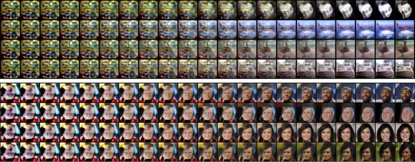
Preprint. Under review
Figure 6: Diagram of AutoN-CODE: Very similarly to a vanilla auto-encoder, the model uses two sets of con-
volutional filters to map the data distribution to a low dimensional representation space. However, rather than
mapping to a to-be-decoded representation, the encoder infers set of control weights parameterizing a linear
system. This data-dependent system is subsequently solved and its last state is used as a low-dimensional rep-
resentation for the decoder reconstruction. The whole architecture remains entirely differentiable and gradients
can be estimated by solving and adjoint state system.
concatenated parameters instantiating the convolution kernels. The 10-class prediction vector is ob-
tained as a linear transformation of the final state x(T ) of the dynamics with a sigmoid activation.
We aimed at simplicity by defining the mapping γ as a two-layer perceptron with 10 hidden units.
We did not perform any fine-tuning, although we did augment the state dimension, akin to ANODE,
by increasing the channel dimension by 10, which helped stabilize training. Results are shown in
Fig. 5.
5.3 U NSUPERVISED LEARNING : I MAGE AUTOENCODING WITH CONTROLLED FLOW
We now use our control approach in an autoencoding model for low-dimensional representation
learning (Fig. 6). Our idea is to invoke a standard class of ordinary differential equations to “encode”
the model’s latent representations, taken as the system state at a fixed point in time.
γµ : U 7→ Θ ⊂ Rn
u 7→ γµ (u) = θ = (θi,j )1≤i,j≤n (7)
The latent code is subsequently interpreted as the solution of the autonomous differential system
presented in equation 8 for a specified time T and given the initial condition (x(0), γµ (u)) with
x(0) a constant initial vector.
dx , dθ = (f (x, θ, t), 0) dx , θ(t) = (hθ , x(t)i, γ (u))
i µ
dt dt = dt (8)
(x(0), θ(0)) = (x(0), γµ (u)) x(0) = (x(0))
This model can be interpreted as a hybrid version of autoencoders and generative normalizing flows,
where the latent generative flow is data-dependent and parametrized by the encoder output. We
found that a simple linear homogeneous differential system was already more expressive than a lin-
ear layer to shape the latent representation. However, since the output dimension of the encoder
grows quadratically with the desired latent code dimension of the bottleneck, we adopted a sparse
prediction strategy, where as few as two elements of each row of (θi,j )1≤i,j≤n are non-zero, making
our model match exactly the number of parameters of a VAE with same architecture. We believe that
the increase in representational power over a vanilla autoencoder, as shown by FID improvements,
despite these simplistic assumptions, shows the potential of this approach for representation learn-
ing (Fig. 9). For the encoder and decoders, we slightly simplify the convolution architecture tested
in (Ghosh et al., 2019; Tolstikhin et al., 2017) and apply batch normalization to all layers (see Ap-
pendix). We make no additional change to the decoder. We train the parameters of the encoder and
6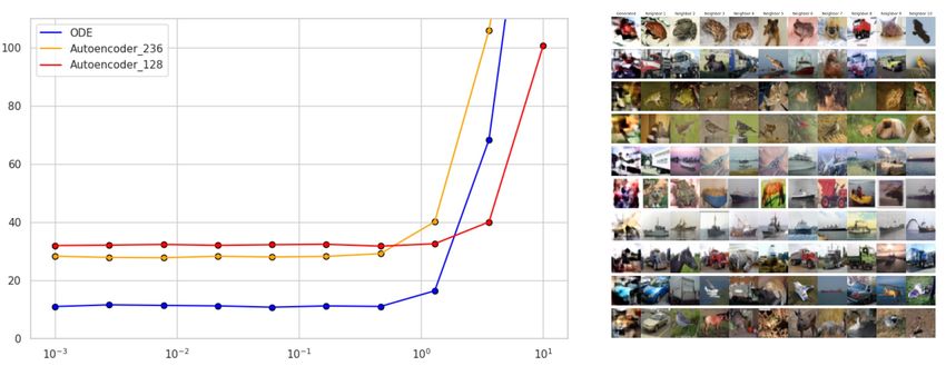
Preprint. Under review

decoder module for minimizing the mean-squared error (MSE) on CIFAR-10 (Krizhevsky, 2012)
and CelebA (Liu et al., 2015) or alternatively the Kullback-Leibler divergence between the data dis-
tribution and the output of the decoder for MNIST (MNI, 1998) (formulas in Appendix.) Gradient
descent is performed for 50 epochs with the Adam (Kingma & Ba, 2014) optimizer with learning
rate λ = 1e−3 reduced by half every time the loss plateaus. All experiments are run on a single
GPU GeForce Titan X with 12 GB of memory.

5.4   I MAGE GENERATION

In order to endow our determinis-
tic model with the ability to gener-
ate image samples, we perform, sim-
ilarly to (Ghosh et al., 2019), a post
hoc density estimation of the distri-
bution of the latent trajectories’ final
state. Namely, we employ a gaussian
mixture model fit with expectation-
maximization, and explore the effect
of increasing the number of com-
ponents in the mixture.          We re-
port in Fig. 9, contrary to (Ghosh
et al., 2019), a substantial decrease of
the Fréchet Inception Distance (FID,
(Heusel et al., 2017)) of our sampled
images to the image test set with in-
creasing number of components in the
mixture (see Fig. 7 for sampled ex-
amples and Fig. 8 for reconstructions
along controlled orbits). These results Figure 7: Random samples generated with AutoN-CODE
suggest, considering the identical ar- trained on CIFAR-10 from a Gaussian Mixture Model with 5000
chitecture of the encoder and decoder components.
to a vanilla model, that the optimal en-
coding control formulation produced a structural change in the latent manifold organization. We
further show that our approach compares favorably to recent generative techniques (see Fig. 10).
Finally, we note that this model offers several original possibilities to explore, such as sampling
from the control coefficients, or adding a regularization on the dynamic evolution as in (Finlay et al.,
2020), which we leave for future work.

6     R ELATED WORK

Figure 8: Left to right: Temporal evolutions of an image reconstruction along controlled orbits of AutoN-
CODE for representative CIFAR-10 and CelabA test images. Last column: ground truth image.

                                                   7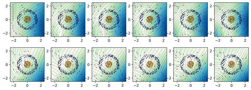
Preprint. Under review

Figure 10: Left Reconstructions of random test images from CelebA for different autoencoding
models. Right: Random samples from the latent space. Deterministic models are fit with 100-
components gaussian mixture model.

Neural ODEs - This work                                                  FID
builds on the recent develop-              Dataset                                                CelebA
ment of Neural ODEs, which              Model                                          CIFAR-10 (64x64)
have shown great promise for            Variational Bayes AE† (Kingma & Welling, 2013) 105.45     68.07
                                        Auto-encoder† (100 components)                 73.24      63.11
building generative normaliz-           PixelCNN (van den Oord et al., 2016)           65.93      -
ing flows (Grathwohl et al.,            Auto-encoder† (1000 components)                55.55      55.60
2018) used for modeling molec-          DCGAN (Radford et al., 2015)                   37.11      -
ular interactions (Köhler et al.,      EBM (10 hist. ensemble) Du & Mordatch (2019) 38.2         -
                                        MoLM (Ravuri et al., 2018)                     33.8       -
2019) or in mean field games            NCSN (Song & Ermon, 2019)                      25.32      -
(Ruthotto et al., 2019). More           SNGAN (Miyato et al., 2018)                    21.7       -
recent work has focused on the          AutoGAN (Gong et al., 2019)                    12.42      -
topological properties of these         AutoNCODE (100 components)                     34.90      55.27
models (Dupont et al., 2019;            AutoNCODE (1000 components)                    24.19      52.47
Zhang et al., 2020), introducing
time-dependent parametrization
                                     Figure 9: Frechet Inception Distance (FID) for several recent architec-
(Zhang et al., 2019b; Mas- tures. (lower is better) Models that are evaluated using authors code are
saroli et al., 2020b; Choroman- noted with †. CelebA results are given for our implementations only as
ski et al., 2020), developing data processing is inconsistent across models.
novel regularization methods us-
ing optimal transport or stochas-
tic perturbations (Finlay et al., 2020; Oganesyan et al., 2020) and adapting them to stochastic differ-
ential equations (Tzen & Raginsky, 2019).
Optimal Control - Several works have interpreted deep learning optimization as an optimal con-
trol problem (Li et al., 2017; Benning et al., 2019; Liu & Theodorou, 2019; Zhang et al., 2019a;
Seidman et al., 2020) providing strong error control and yielding convergence results for alternative
algorithms to standard gradient-based learning methods. Of particular interest is the mean-field opti-
mal control formulation of (E et al., 2018), which notes the dependence of a unique control variable
governing the network dynamics on the whole data population.
Hypernetworks - Finally, this work is also related to network architectures with adaptive weights
such as Hypernetworks (Ha et al., 2016), dynamic filters (Brabandere et al., 2016) and spatial trans-
formers (Jaderberg et al., 2015). Though not explicitly formulated as optimal neural control, these
approaches effectively implement a form of modulation of neural network activity as a function of
input data and activation state, resulting in compact and expressive models. These methods demon-
strate, in our opinion, the significant untapped potential value in developing dynamically controlled
modules for deep learning.

7    C ONCLUSION

In this work, we have presented an original control formulation for continuous-time neural feature
transformations. We have shown that it is possible to dynamically shape the trajectories of the trans-
formation module applied to the data by augmenting the network with a trained control inference
mechanism, and further demonstrated that this can be applied in the context of supervised and unsu-

                                                     8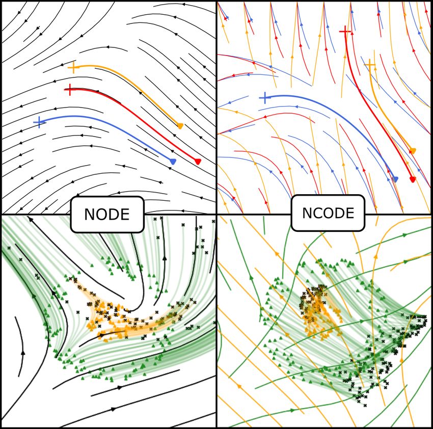
Preprint. Under review

pervised image representation learning. In future work, we would like to investigate the robustness
and generalization properties of such controlled models as well as their similarities with fast-synaptic
modulation systems observed in neuroscience, and test this on natural applications such as recurrent
neural networks and robotics. An additional avenue for further research is the connection between
our system and the theory of bifurcations in dynamical systems and neuroscience.

                                                   9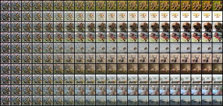
Preprint. Under review

R EFERENCES
”gradient-based learning applied to document recognition.”. Proceedings of the IEEE, 1998.
Martin Benning, Elena Celledoni, Matthias J. Ehrhardt, Brynjulf Owren, and Carola-Bibiane
 Schönlieb. Deep learning as optimal control problems: models and numerical methods, 2019.
Bert De Brabandere, Xu Jia, Tinne Tuytelaars, and Luc Van Gool. Dynamic filter networks, 2016.
Ricky T. Q. Chen, Yulia Rubanova, Jesse Bettencourt, and David Duvenaud. Neural ordinary dif-
  ferential equations, 2018.
Krzysztof Choromanski, Jared Quincy Davis, Valerii Likhosherstov, Xingyou Song, Jean-Jacques
  Slotine, Jacob Varley, Honglak Lee, Adrian Weller, and Vikas Sindhwani. An ode to an ode, 2020.
A. P. Dempster, N. M. Laird, and D. B. Rubin. Maximum likelihood from incomplete data via the
  em algorithm. Journal of the Royal Statistical Society. Series B (Methodological), 39(1):1–38,
  1977. ISSN 00359246. URL http://www.jstor.org/stable/2984875.
Yilun Du and Igor Mordatch. Implicit generation and generalization in energy-based models, 2019.
Emilien Dupont, Arnaud Doucet, and Yee Whye Teh. Augmented neural odes, 2019.
Weinan E, Jiequn Han, and Qianxiao Li. A mean-field optimal control formulation of deep learning,
 2018.
Chris Finlay, Jörn-Henrik Jacobsen, Levon Nurbekyan, and Adam M Oberman. How to train your
  neural ode: the world of jacobian and kinetic regularization, 2020.
Partha Ghosh, Mehdi S. M. Sajjadi, Antonio Vergari, Michael Black, and Bernhard Schölkopf. From
  variational to deterministic autoencoders, 2019.
Xinyu Gong, Shiyu Chang, Yifan Jiang, and Zhangyang Wang. Autogan: Neural architecture search
  for generative adversarial networks, 2019.
Will Grathwohl, Ricky T. Q. Chen, Jesse Bettencourt, Ilya Sutskever, and David Duvenaud. Ffjord:
 Free-form continuous dynamics for scalable reversible generative models, 2018.
Will Grathwohl, Ricky T. Q. Chen, Jesse Bettencourt, and David Duvenaud. Scalable reversible
 generative models with free-form continuous dynamics. In International Conference on Learning
 Representations, 2019. URL https://openreview.net/forum?id=rJxgknCcK7.
David Ha, Andrew Dai, and Quoc V. Le. Hypernetworks, 2016.
Jack K Hale. Dynamical systems and stability. Journal of Mathematical Analysis and Applications,
  26(1):39 – 59, 1969. ISSN 0022-247X. doi: https://doi.org/10.1016/0022-247X(69)90175-9.
Kaiming He, Xiangyu Zhang, Shaoqing Ren, and Jian Sun. Deep residual learning for image recog-
  nition, 2015.
Martin Heusel, Hubert Ramsauer, Thomas Unterthiner, Bernhard Nessler, and Sepp Hochreiter.
 Gans trained by a two time-scale update rule converge to a local nash equilibrium, 2017.
Max Jaderberg, Karen Simonyan, Andrew Zisserman, and Koray Kavukcuoglu. Spatial transformer
 networks, 2015.
Diederik P. Kingma and Jimmy Ba. Adam: A method for stochastic optimization, 2014.
Diederik P Kingma and Max Welling. Auto-encoding variational bayes, 2013.
Alex Krizhevsky. Learning multiple layers of features from tiny images. University of Toronto, 05
  2012.
Jonas Köhler, Leon Klein, and Frank Noé. Equivariant flows: sampling configurations for multi-
  body systems with symmetric energies, 2019.

                                               10
Preprint. Under review
Qianxiao Li, Long Chen, Cheng Tai, and Weinan E. Maximum principle based algorithms for deep
learning, 2017.
Hongzhou Lin and Stefanie Jegelka. Resnet with one-neuron hidden layers is a universal approxi-
mator, 2018.
Guan-Horng Liu and Evangelos A. Theodorou. Deep learning theory review: An optimal control
and dynamical systems perspective, 2019.
Ziwei Liu, Ping Luo, Xiaogang Wang, and Xiaoou Tang. Deep learning face attributes in the wild.
In Proceedings of International Conference on Computer Vision (ICCV), December 2015.
Stefano Massaroli, Michael Poli, Michelangelo Bin, Jinkyoo Park, Atsushi Yamashita, and Hajime
Asama. Stable neural flows, 2020a.
Stefano Massaroli, Michael Poli, Jinkyoo Park, Atsushi Yamashita, and Hajime Asama. Dissecting
neural odes, 2020b.
Takeru Miyato, Toshiki Kataoka, Masanori Koyama, and Yuichi Yoshida. Spectral normalization
for generative adversarial networks, 2018.
Viktor Oganesyan, Alexandra Volokhova, and Dmitry Vetrov. Stochasticity in neural odes: An
empirical study, 2020.
Adam Paszke, Sam Gross, Francisco Massa, Adam Lerer, James Bradbury, Gregory Chanan, Trevor
Killeen, Zeming Lin, Natalia Gimelshein, Luca Antiga, Alban Desmaison, Andreas Köpf, Ed-
ward Yang, Zach DeVito, Martin Raison, Alykhan Tejani, Sasank Chilamkurthy, Benoit Steiner,
Lu Fang, Junjie Bai, and Soumith Chintala. Pytorch: An imperative style, high-performance deep
learning library, 2019.
Gamkrelidze R V Pontryagin Lev Semyonovich ; Boltyanskii V G and Mishchenko E F. The math-
ematical theory of optimal processes. 1962.
Alec Radford, Luke Metz, and Soumith Chintala. Unsupervised representation learning with deep
convolutional generative adversarial networks, 2015.
Suman Ravuri, Shakir Mohamed, Mihaela Rosca, and Oriol Vinyals. Learning implicit generative
models with the method of learned moments, 2018.
Lars Ruthotto, Stanley Osher, Wuchen Li, Levon Nurbekyan, and Samy Wu Fung. A machine learn-
ing framework for solving high-dimensional mean field game and mean field control problems,
2019.
Lars Ruthotto, Stanley J. Osher, Wuchen Li, Levon Nurbekyan, and Samy Wu Fung. A machine
learning framework for solving high-dimensional mean field game and mean field control prob-
lems. Proceedings of the National Academy of Sciences, 117(17):9183–9193, 2020. ISSN 0027-
8424. doi: 10.1073/pnas.1922204117. URL https://www.pnas.org/content/117/
17/9183.
Jacob H. Seidman, Mahyar Fazlyab, Victor M. Preciado, and George J. Pappas. Robust deep learning
as optimal control: Insights and convergence guarantees. volume 120 of Proceedings of Machine
Learning Research, pp. 884–893, The Cloud, 10–11 Jun 2020. PMLR.
Yang Song and Stefano Ermon. Generative modeling by estimating gradients of the data distribution,
2019.
Ilya Tolstikhin, Olivier Bousquet, Sylvain Gelly, and Bernhard Schoelkopf. Wasserstein auto-
encoders, 2017.
Belinda Tzen and Maxim Raginsky. Neural stochastic differential equations: Deep latent gaussian
models in the diffusion limit, 2019.
Aaron van den Oord, Nal Kalchbrenner, Oriol Vinyals, Lasse Espeholt, Alex Graves, and Koray
Kavukcuoglu. Conditional image generation with pixelcnn decoders, 2016.
11Preprint. Under review
Dinghuai Zhang, Tianyuan Zhang, Yiping Lu, Zhanxing Zhu, and Bin Dong. You only propagate
once: Accelerating adversarial training via maximal principle. In H. Wallach, H. Larochelle,
A. Beygelzimer, F. dÁlché Buc, E. Fox, and R. Garnett (eds.), Advances in Neural Information
Processing Systems 32, pp. 227–238. Curran Associates, Inc., 2019a.
Han Zhang, Xi Gao, Jacob Unterman, and Tom Arodz. Approximation capabilities of neural odes
and invertible residual networks, 2020.
Tianjun Zhang, Zhewei Yao, Amir Gholami, Joseph E Gonzalez, Kurt Keutzer, Michael W Ma-
honey, and George Biros. Anodev2: A coupled neural ode framework. In H. Wallach,
H. Larochelle, A. Beygelzimer, F. dÁlché Buc, E. Fox, and R. Garnett (eds.), Advances in Neural
Information Processing Systems 32, pp. 5151–5161. Curran Associates, Inc., 2019b.
12Preprint. Under review
A A PPENDIX
A.1 P ROOF OF T HEOREM 1
Proof. The proof is inspired from Massaroli et al. (2020a). We place our analysis in the Banach
space Rn . Since ` and h are continuously differentiable,
let us form the Lagrangian functional L
x
where a is an element of the dual space of z = :
θ
ZT
∂z
L(z, a, t) := [` − ha, − hi]dt (9)
∂t
0
∂z
The constraint ha(t), − h(z, t)i is always active on the admissible set by construction of z in
∂t
∂L ∂l
equation 4, such that we have ∀z, a, (z, a, t) = (z, a, t). Moreover, integrating the left
∂µ ∂µ
part of the integral in equation 9 gives:
ZT ZT
∂z T ∂a
ha, idt = ha, zi 0
− h , zidt (10)
∂t ∂t
0 0
da
Now, given that ` − h , zi is derivable in µ for any t ∈ [0, T ], Leibniz integral rule allows to write
dt
ZT
∂l ∂ da ∂z(T ) ∂z(0)
[` + h , zi + ha, hi]dt + ha(T ), i − ha(0), i
= (11)
∂µ ∂µ dt ∂µ ∂µ
0
ZT
∂l ∂` ∂z da ∂z ∂h ∂z(T )
= [ +h , i + ha, i]dt + ha(T ), i (12)
∂µ ∂z ∂µ dt ∂µ ∂µ ∂µ
0
ZT
∂l ∂` ∂z da ∂z ∂h ∂h ∂t
∂h ∂z ∂z(T )
+h , i + ha, ]dt + ha(T ), i
= [ + + (13)
∂µ ∂z ∂µ dt ∂µ ∂µ ∂t ∂µ ∂z ∂µ ∂µ
0
The last equation can be reordered as:
ZT ZT
∂l da ∂h ∂` ∂z ∂h ∂z(T )
= h −a − , idt + ha, idt + ha(T ), i (14)
∂µ dt ∂z ∂z ∂µ ∂µ ∂µ
0 0
da ∂h ∂` ∂z
Posing that a(T ) = O|X |+|Θ| and h −a − , i = 0, the result follows.
dt ∂z ∂z ∂µ
Remark 1: This result allows to compute gradient estimate assuming that µ directly parametrizes
∂h
h such that the gradient are straightforward to compute. However, in the case of optimizing
∂µ
the initial mapping γ that infer the variable θ , this result can be combined with usual chain rule to
estimate the gradient:
∂l ∂θ ∂l
= (15)
∂µγ ∂γ ∂θ
13Preprint. Under review
A.2 I MPLEMENTATION
Generic N-CODE module - We provide here a commented generic PyTorch implementation for
the N-CODE module in the open-loop setting.
1
2
3 class NCODE(torch.autograd.Function):
4 @staticmethod
5 def forward(ctx, x_t, theta_t, t, model, control, model_names,
parameters_size, device, *adjoint_params):
6 """
7 - ctx : context object that can be used to stash information for
backward computation.
8 - z_t : the tuple of tensors representing the state and controls
of the system
9 - model_names, parameters_size : arguments to initiate the model
update
10
11 """
12 ### 1) Instantiate f_model with control parametrization
13 state_dict = OrderedDict(zip(model_names,\theta_t))
14 model.load_state_dict(state_dict)
15 d_x = model(y_t)
16
17 ### 2) Compute control update as per equation dw/dt =
18 d_u = control(y_t)
19
20 ### 3) return dz/dt = [dx/dt, dtheta_1/dt, ..., dtheta_N/dt]
21 dz = (d_y, *d_u)
22
23 ### 4) Save models and tensors
24 ctx.save_for_backward(h, d_x, x_t, *\theta_t)
25 ctx.model_names = model_names
26 ctx.parameters_size = parameters_size
27 ctx.device = device
28 ctx.intermediate = d_theta , theta_t
29 ctx.theta_t = theta_t
30 ctx.model = model
31 ctx.control = control
32
33 return dz
34
35 @staticmethod
36 def backward(ctx, grad_out, a=None, b=None, c=None, d=None):
37 """
38 - grad_out : Tensor (or tuple of tensors) containing the
gradient of the loss
39 function with respect to y_t and u_t
40
41 """
42
43 with torch.no_grad():
44 grad_x_out = grad_out
45 h, d_x, x_t, *theta_t = ctx.saved_tensors
46 model = ctx.model
47 control = ctx.control
48 model_names = ctx.model_names
49 parameters_size = ctx.parameters_size
50
51 state_dict = OrderedDict(zip(model_names, theta_t))
52 model.load_state_dict(state_dict)
53 grad_weigths = [torch.zeros_like(param) for param in tuple(
ctx.control.parameters())]
54
14Preprint. Under review
55 with torch.enable_grad():
56 model_eval = model(x_t)
57 control_eval = [layer(control[1](control[0](x_t))).
reshape(parameters_size[i]) for i, layer in enumerate(control[2:])]
58 control_eval_param = [nn.Parameter(weight,requires_grad=
True) for weight in control_eval]
59
60 #compute jacobian for f_model
61
62 d_mod_dx, *d_mod_dtheta = torch.autograd.grad(model_eval,
(x_t,) + tuple(ctx.model.parameters()), grad_x_out, create_graph=
False)
63
64 for i, grad_u in enumerate(d_mod_du):
65 d_con_dmu = torch.autograd.grad(control_eval[i],
tuple(ctx.control.parameters()), grad_theta, create_graph=False,
retain_graph=True, allow_unused=True)
66 grad_weigths = [ grad_weigths[i] + d_con_dmu[i] if
d_con_dmu[i] is not None else grad_weigths[i] for i in range(len(
d_con_dmu))]
67 d_con_du = None
68
69
70 grad_y_in = d_mod_dy
71 adj_params = grad_weigths
72
73 return (grad_y_in, None, None, None, None, None, None, None, *
adj_params)
Listing 1: Generic N-CODE module forward and backward methods
A.3 E XPERIMENTAL RESULTS
Resources - Our experiments were run on a 12GB NVIDIA® Titan Xp GPUs cluster equipped
with CUDA 10.1 driver. Neural ODEs were trained using torchdiffeq (Chen et al., 2018) PyTorch
package.
A.4 F LOWS FOR ANNULI DATASET
Figure A.1: Time-varying flows for two class-different points of the annuli dataset.
A.5 AUTO N-CODE ARCHITECTURES
Adapting the models adopted by Tolstikhin et al. (2017) and Ghosh et al. (2019), we use a latent
space dimension of 25 for MNIST, 128 for CIFAR-10 and 64 for CelebA. All convolutions and
transposed convolutions have a filter size of 4×4 for MNIST and CIFAR-10 and 5×5 for CELEBA.
15Preprint. Under review
MNIST CIFAR-10 CelebA
3×28×28 3×32×32
x∈R x∈R x ∈ R3×64×64
Encoder: Flatten Conv256 7→ BN 7→ Relu Conv256 7→ BN 7→ Relu
FC400 7→ Relu Conv512 7→ BN 7→ Relu Conv512 7→ BN 7→ Relu
FC25 7→ Norm Conv1024 7→ BN 7→ Relu Conv1024 7→ BN 7→ Relu
FC128∗2 7→ Norm FC64∗10 7→ Norm
Latent dynamics: ODE[0,10] ODE[0,10] ODE[0,10]
Decoder: FC400 7→ Relu FC1024∗8∗8 7→ Norm FC1024∗8∗8 7→ Norm
FC784 7→ Sigmoid ConvT512 7→ BN 7→ Relu ConvT512 7→ BN 7→ Relu
ConvT256 7→ BN 7→ Relu ConvT256 7→ BN 7→ Relu
ConvT3 ConvT3
Table A.1: Model architectures for the different data sets tested. FCn and Convn represents respec-
tively fully connected and convolutional layer with n output/filters. We apply a component-wise
normalisation of the controls components which proved crucial for good performance of the model.
The dynamic is ran on the time segment [0,10] which empirically yield good results.
They all have a stride of size 2 except for the last convolutional layer in the decoder. We use Relu
non-linear activation and batch normalisation at the end of every convolution filter. Official train
and test splits are used for the three datasets. For training, we use a mini-batch size of 64 in MNIST
and CIFAR and 16 for CelebA in AutoN-CODE. (64 for control models.) All models are trained
for a maximum of 50 epochs on MNIST and CIFAR and 40 epochs on CelebA.
A.6 V ISUALIZATION OF LATENT CODE DYNAMICAL EVOLUTION
Figure A.2: Reconstructions of the image along the controlled orbits of AutoN-CODE for MNIST.
The temporal dimension reads from left to right. Last column: ground truth image
A.7 E XPLORING SAMPLING DISTRIBUTIONS
For random samples evaluation, we train the VAE with a N (0, I) prior. For the deterministic models,
samples are drawn from a mixture of multivariate gaussian distributions fitted using the testing
set embeddings. The distribution is obtained through Expectation-Maximization Dempster et al.
(1977) with one single k-means initialization, tolerance 1e−3 and run for at most 100 iterations.
We compute the FID using 10k generated samples evaluated against the whole test set for all FID
16Preprint. Under review
Figure A.3: Reconstructions of the image along the controlled orbits of AutoN-CODE for CIFAR-
10. The temporal dimension reads from left to right. Last column: ground truth image.
Figure A.4: Reconstructions of the image along the controlled orbits of AutoN-CODE for CelebA.
The temporal dimension reads from left to right. Last column: ground truth image
evaluations, using the standard 2048-dimensional final feature vector of an Inception V3 following
Heusel et al. (2017) implementation.
Further experiments showed that 10K components (matching the number of data points in the test
sets) logically overfits on the data distribution. Generated images display marginal changes com-
pared to test images. However, 1000 components does not, showing that our AutoN-CODE sampling
strategy describe a trade-off between sample quality and generalization of images. We alternatively
tested non-parametric kernel density estimation with varying kernel variance to replace our initial
sampling strategy. We report similar result to gaussian mixture with an overall lower FID of AutoN-
CODE for small variance kernels. As the fiting distribution becomes very rough (σ ∼ 5), the
generated image quality is highly deteriorating.(see Figure S6).
17Preprint. Under review
Figure A.5: Nearest neighbors search of random samples from the gaussian mixture with (Left)
1000 components (Left) and (Right) 10K components in the testing set of CIFAR-10.
Figure A.6: (Left) Evolution of FID between test set and generated samples as a function of the gaus-
sian kernel variance used to perform kernel estimation of the the latent code distribution. (Right)
Nearest neighbors search of random samples from the latent distribution fitted with a gaussian kernel
estimation with variance σ = 2 in the testing set.
A.8 L ATENT CODE INTERPOLATION
18Preprint. Under review
Figure A.7: t-SNE embeddings of the latent code at t = t1 for MNIST test set colored with a 10
component gaussian mixture model.
19Preprint. Under review
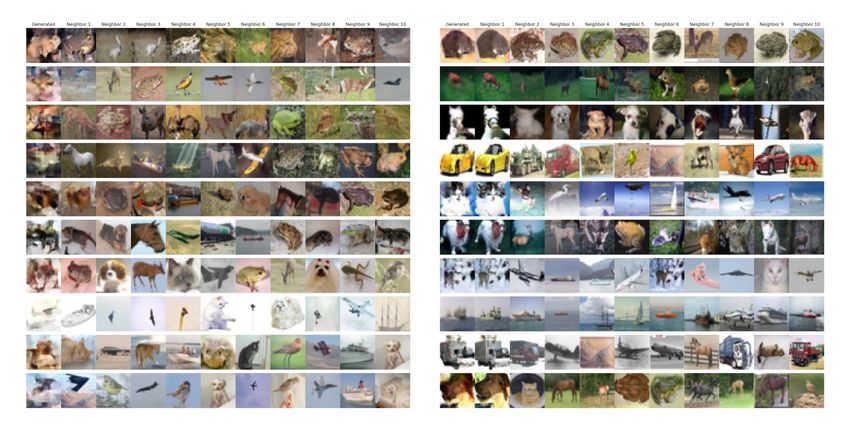
Figure A.8: Interpolation: We further explore the latent space of AutoN-CODE by interpolating
between the latent vectors of the CelebA test set. (Upper panel) Linear interpolation between ran-
dom samples reconstructed with AutoN-CODE. (Middle panel) Interpolation comparison between
AutoN-CODE and a vanilla auto-encoder for a single pair of vectors. (Lower panel) 2d interpo-
lation with three anchor reconstructions corresponding to the three corners of the square (A:up-
left,B:up-right and C:down-left. Left square corresponds to AutoN-CODE reconstructions and right
to a vanilla auto-encoder.
20You can also read