GPU-based Steady-State Solution of the Chemical Master Equation
←
→
Page content transcription
If your browser does not render page correctly, please read the page content below
GPU-based Steady-State Solution of the Chemical Master Equation

                                      Marco Maggioni, Tanya Berger-Wolf, Jie Liang
                               Department of Computer Science, Department of Bioengineering
                                              University of Illinois at Chicago
                                        Email: {mmaggi3,tanyabw,jliang}@uic.edu

   Abstract—The Chemical Master Equation (CME) is a                basic principles on how biological networks function and
stochastic and discrete-state continuous-time model for macro-     how they respond to various environmental perturbations,
molecular reaction networks inside the cell. Under this theoret-   having critical applications in stem cell study and cancer
ical framework, the solution of a sparse linear system provides
the steady-state probability landscape over the molecular          development.
microstates. The CME framework can in fact reveal important           Under the CME framework, a stochastic characteriza-
insights into basic principles on how biological networks          tion of the biochemical system is provided by a time-
function, having critical applications in stem cell study and      varying probability landscape over microstates representing
cancer development. However, the exploratory nature of system      the detailed chemical amount of each and every molecular
biology research involves the solution of the same reaction
network under different conditions. As a result, the application   species. The stationary behavior at the limit can be analyzed
of the CME framework is feasible only if we are able to solve      to identify biologically meaningful macrostates. This step
several large linear systems in a reasonable amount of time.       involves the solution of a sparse linear system of equations
   In recent years, GPU has emerged as a cost-effective            representing stochastic microstate transitions. Despite the
high performance architecture easily available to bioscientists    assumption of small copy numbers in a cell, the CME
around the world. In this paper, we propose an efficient GPU-
based Jacobi iteration for steady-state probability calculation.   framework poses a computational challenge when applied
We provide several optimization strategies based on the prob-      to realistic systems due to an exponential growth in the
lem structure with the aim of outperforming the conventional       number of microstates [2]. Moreover, the exploratory nature
multicore implementation while minimizing the GPU memory           of system biology research involves the study of the same
footprint. We combine an ELL+DIAG sparse matrix format             reaction network under different conditions (e.g. varying the
with DFS ordering to leverage the diagonal density. Moreover,
we devise an improved sliced ELL sparse matrix representation      intrinsic rate of one of the involved reactions). The compu-
based on warp granularity and local rearrangement.                 tational demands may become overwhelming and, hence,
   Experimental results demonstrate an average double-             practically infeasible for computer architectures based on
precision performance of 14.212 GFLOPS in solving the CME          a limited number of parallel processing elements such as
(a speedup of 15.67x compared to the optimized Intel MKL           conventional multicore CPUs. This observation motivates the
library). Our implementation of the warp-grained sliced ELL
format outperforms the state-of-the-art in terms of SpMV           use of high performance computer architectures to solve the
performance (a speedup of 1.24x over clSpMV). Moreover, it         steady-state probability landscape problem.
shows consistent improvements for a wider set of application          Over the past years, GPUs have evolved from an
domains and a good memory footprint reduction. The results         application-specific processors dedicated to 3D visualization
achieved in this work provide the foundation for applying the      into a more general purpose parallel platform available for
CME framework to realistic biochemical systems. In addition,
our GPU-based steady-state computation can be generalized to       scientific computing. Bioscientists around the world can
operation on stochastic matrices (Markov models), achieving        easily have access to this high performance architecture
good performance with matrix structures similar to biological      due its cost-effectiveness. As a consequence, the solution of
reaction networks.                                                 increasingly complex scientific problems can be computed in
   Keywords-GPU; sparse linear algebra; chemical master            practice, advancing science in novel directions. The station-
equation; system biology; Jacobi iteration; computational bi-      ary analysis of biochemical reaction network can certainly
ology;                                                             benefit of the high floating-point throughput and memory
                                                                   bandwidth peaks offered by modern GPU architecture like
                     I. I NTRODUCTION                              Fermi [3]. Specifically, the availability of a large memory
   Networks of interacting biomolecules are at the heart of        bandwidth permits to mitigate the bandwidth-bound nature
the regulation of cellular processes, and stochasticity plays      of sparse linear algebra operations necessary to calculate
important roles. The Chemical Master Equation (CME) [1]            the CME solution. Due to the centrality of linear algebra
is a stochastic and discrete-state continuos-time formulation      in scientific and engineering computations, a large research
that provides a fundamental framework to model biochemi-           effort has been dedicated to improve efficiency and memory
cal reaction networks inside the cells. In general, an accurate    representation compactness of GPU-based Sparse Matrix-
solution to the CME can reveal important insights into             Vector multiplication (SpMV) [4, 5, 6, 7, 8]. This body of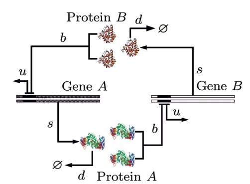
work can be taken as foundation for implementing the Jacobi            to reach an average double-precision performance of
iteration [9], a well-known and easy-to-parallelize iterative          14.212 GFLOP/s and a speedup of 15.67x compared to
method for solving linear systems.                                     the optimized Intel MKL library [14].
   In this paper, we propose an efficient GPU-based Jacobi         •   An improved sliced ELL sparse matrix representation
iteration for steady-state probability landscape calculation.          based on warp granularity and local rearrangement. We
Similarly to what done in [10] for graph mining, we analyze            are able to show that this optimized format outperforms
the structure of problems arising from the CME and we                  the state-of-the-art in terms of SpMV performance on
provide several optimization strategies with the aim of out-           matrices arising from the CME framework (a speedup
performing the conventional multicore implementation while             of 1.24x over clSpMV [15], a framework capable of
minimizing the GPU memory footprint. First, the transition             selecting the best representation of any sparse matrix).
matrix can be efficiently represented using the ELL format             Considering a wider set of application domains, the
[4] due to a limited number of possible reactions for each             warp-grained ELL format has consistent improvements
microstate. Second, it is possible to take advantage of                compared to the original sliced ELL format. More-
reversible reactions in order to improve the diagonal density          over, it minimizes the footprint of the underlying data
of the transition matrix. Specifically, the DFS ordering of            structure (a relevant factor due to the limited memory
the microstates exposes a densely populated band composed              available on current GPU devices).
by the main diagonal and its two immediate neighbors. We            The structure of the paper is as follows. Section II
can leverage this structure by separately storing the dense      introduces the theoretical background of the CME. Section
diagonals using the DIA format [4]. In this paper, we also       III presents a brief description of the GPU architecture.
propose a novel sparse matrix representation that optimizes      Section IV introduces the Jacobi iterative method. Section
the sliced ELL format presented in [5]. The basic idea is        V provides a detailed analysis of the problem structure and
to reduce as much as possible the overhead associated with       devises some domain-specific GPU optimizations whereas
the data structure. This goal is achieved by following two       Section VI describes the novel warp-grained ELL format.
strategies. First, the slice size is chosen in order to match    Performance results of the various optimization strategies are
the execution block in hardware (warp). Second, we apply         then given in Section VII. Finally, Section VIII is devoted
a local rearrangement that uniforms the number of nonzeros       to conclusions.
within each slice and improves the data structure efficiency
without deteriorating the cache locality. This warped-grained
                                                                           II. T HE C HEMICAL M ASTER E QUATION
sliced ELL can be also combined with the DIA optimization,
at least when the local rearrangement does not decrease too         In the theory of the Chemical Master Equation, the dy-
much the diagonal density.                                       namics of a biochemical reaction system, in a small volume,
   The use of GPUs to solve large Markov models, a topic         is represented by a discrete-state continuous-time Markov
close to the research presented in this paper, has been dis-     process and is characterized by a probability distribution as
cussed in previous literature. The authors of [11] implements    function of time. The CME basically describes the change of
a GPU-based Jacobi iteration. Besides being limited by           probability of different microstates connected by reactions.
an out-of-date GPU architecture, their work is based on
the general CSR format [12] and does not propose any             A. Stochastic framework
optimization strategy. Analogously, the authors of [13] do
not introduce any significant contribution other than testing       The state space of the CME is represented by a de-
well-known GPU-based SpMV kernels on some matrices               tailed amount of each and every of the m molecular
derived from Markov models. The novelty of this paper            species in the biochemical reaction network. The microstate
lies in specific GPU optimization strategies to achieve better   of the system at time t is then defined as x(t) =
performance and memory footprint. Moreover, we propose           {x1 (t), x2 (t), ..., xm (t)} ∈ Nm and the overall state space
the first practical implementation of the CME stochastic         is the set X of all possible combination numbers X =
framework. The ability to study realistic cellular reaction      {x(t)|t ∈ (0, ∞)}. A fundamental characterization of the
networks opens up a new direction of biological computing        system is given by the collection of probabilities P(t) ∈
that will be, without exaggeration, every bit as important as    [0, 1]|X | for each of the microstate at time t. P(t) is defined
molecular dynamics simulation. The specific contributions        as the probability landscape.
                                                                                                                       k
of this work are the followings:                                    The transition rates between microstates (xj −→ xi ) con-
   • An efficient GPU-based Jacobi iteration for steady-state    nected by the k-th reaction are determined by the intrinsic
      probability calculation of biological reaction networks,   reaction rate rk and by reactants involved
      which can be generalized to operation on stochastic                                                           m
      matrices (Markov models). On a dataset of transition
                                                                                                                   Y     xi
                                                                       Ak (xi , xj ) = Ak (·, xj ) = Ak (xj ) = rk
      matrices derived from biological models, we were able                                                        i=1
                                                                                                                         ci
where ci is the copy number of species i needed to perform
the reaction (Ak (xi , xj ) > 0 when two microstates are con-
nected by the k-th reaction, Ak (xi , xj ) = 0 otherwise). In
principle, the transition xj −→ xi between two microstates
can correspond to different reactions, so the overall reaction
rate is X
A(xi , xj ) = Ak (xi , xj )
k∈R
The discrete Chemical Master Equation can then be
written as
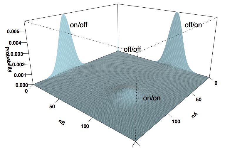
Figure 1. Model of a toggle switch [17]
dP(x, t) Xh i
= A(x, x0 )P(x0 , t) − A(x0 , x)P(x, t)
dt 0x 6=x
where P(x, t) is the probability in continuous time of a dis-
crete microstate. The gain and loss of probability associated
with each microstate is a balance between the incoming and
the outcoming reaction rates. The CME can also be written
in a more compact form by defining the rate constant for
leaving the current state A(x, x) as
X
A(x, x) = − A(x0 , x)
x0 6=x
Consequently, the probability landscape variation can be
described in the following matrix-vector form
dP(t) Figure 2. Steady state probability landscape of a toggle switch [17]
= AP(t)
dt
where A ∈ R|X |×|X | is a sparse reaction rate matrix formed
and the macroscopic behavior of the biochemical reaction
by the collection of all A(xi , xj ).
network. Specifically, the probability is concentrated around
B. Steady-state probability landscape the states with mutual inhibition (“on/off” and “off/on”)
The stationary behavior of this stochastic model can where only copies of one protein (nA or nB) are present.
provide biological insight about the underlying biochemical A reliable stochastic model of the reaction network re-
reaction network. Given the reaction rate matrix A, the quires a complete identification of the microstates. The
steady-state probability landscape P over the microstates is corresponding state space X considers all the possible
directly derived from the CME as combination numbers and grows exponentially with the
number m of molecular species. A rough bound for this
dP(t) state space size is given by |X | ≤ k m , where k is the
= AP = 0
dt maximum copy number for each species. However, it might
Intuitively, the steady-state corresponds to the condition be argued that the structure of the reaction network limits the
dP(t)
dt = 0. Therefore, we can derive P by solving the microstates effectively reachable from an initial condition.
correspondent system of linear equations AP = 0. This intuition has been used in [17] to produce a minimal
We can show an example of the CME stochastic frame- and comprehensive state space X . Specifically, it is possible
work use. We consider the well-studied genetic toggle to identify a graph structure where microstates are nodes
system [16], a network composed by two genes A and B and reactions are edges. A DFS visit starts from an initial
arranged in mutual inhibition. This model is depicted in microstate and produces the reachable subspace X , along
Figure 1. The intuitive bistable behavior would see one with the associated reaction rate matrix A.
gene synthesizing its protein (gene “on”) while the other The concrete application of the CME stochastic frame-
is inhibited (gene “off”). The analysis of the steady-state work is not a trivial task. First, the arising linear systems
probability landscape should provide an insight of such are intrinsically ill-conditioned posing numerical problems
bistability. Hence, we can solve the linear system AP = 0 during the solution. Second, the size n = |X | quickly
in order to derive the landscape shown in Figure 2. In this poses a practical feasibility issue for computer architectures
example, the CME stochastic framework is able to provide with limited parallelism. Last, bioscientists usually study a
a connection between the microstate probability distribution reaction network under different conditions. Considering thateach combination of the parameters generates a different accesses).
linear system, the total amount of computation may become Despite the availability of a large memory bandwidth,
excruciatingly large. algorithms with low arithmetic intensity are able to achieve
only a fraction of the theoretical performance peak. The
III. GPU ARCHITECTURE Fermi architecture implements a fused multiple-add (FMA)
The architecture of modern GPUs has evolved into a instruction for which two floating point operations are ex-
general purpose parallel platform optimized for computing- ecuted in a single cycle. Considering a bandwidth of 192
intensive data processing. The idea of hardware multithread- GB/s and the need of loading double-precision operands
ing is central for this architecture. In brief, the availabil- from global memory, we can perform at most 12 GFLOPS
ity of a large pool of threads ready to execute (coupled (each FMA needs 4 doubles, or 32 bytes). This perfor-
with fast context switching) can keep functional units busy mance is way below to the Fermi architecture theoretical
and hide memory accesses. Hence, the use of large and peak (≈ 789 GB/s). It might be also argued that gaming-
complex cache memories becomes less crucial and more oriented GPUs (such a GTX580) have a performance edge
silicon area can be dedicated to implement computational over computing-oriented GPUs (such as Tesla) for double-
cores. In this subsection we describe the key aspects of precision sparse linear algebra. In more detail, GTX580
NVIDIA Fermi architecture [3]. We refer to this particular offers a larger bandwidth despite having a double-precision
architecture because our experimental results are based on performance peak locked at one-quarter of the chip’s peak
the CUDA programming model [18] and on the specific potential (≈ 197 GFLOPS). Hence, it can potentially offer
NVIDIA GTX580 device . a better performance for bandwidth-limited algorithms such
A GPU is composed by a number of processing units as sparse linear algebra.
called Streaming Multiprocessors (SMs), each one contain- CUDA is an abstract parallel computing architecture and
ing a set of simple computing cores known as Streaming programming model based on few concepts. First, there
Processors (SPs) or CUDA cores. Referring to GTX580, exists a hierarchy of concurrent lightweight threads to model
we have 16 SMs with 32 SPs each for a total of 512 the computation according to a data-parallel model. In brief,
cores (a potential parallelism of 512 operations for clock the algorithm should be expressed in such a way each data
cycle). The execution of instructions within SMs follows the element is processed by an independent lightweight thread.
single-instruction multiple-thread (SIMT) model with warp All threads execute the same program on different data.
granularity (32 threads). Whenever threads within the same Threads are logically grouped into equally sized blocks.
warp needs to execute a different branch of instructions, Cooperation and synchronization within blocks are allowed
we have a divergence and the execution is serialized with by the means of shared memory and primitives. Finally,
intrinsic performance decreasing. blocks are grouped into a grid for covering all the data
SMs are connected to a random access memory through to process. This hierarchy represents an abstraction of the
a cache hierarchy. This global memory has high bandwidth underlying GPU architecture. Specifically, blocks represent
(192 GB/s for GTX580) but high latency (up to 800 clock abstract SMs capable to run all the threads simultaneously.
cycles). The cache hierarchy is organized on two levels. A However, a block is permanently assigned to one of the
coherent L2 cache (768 KB) is shared among all the SMs available SMs and executed as warps in an arbitrary order.
and provides a mean to reduce the global memory bandwidth This approach assures scalability since CUDA code can be
usage (whereas latency is not improved). Each SM also compiled and executed on devices with different number of
has a local on-chip memory (64KB) with low latency and multiprocessors. Referring to GTX580, each SM can manage
very high bandwidth (≈ 3.15 TB/s). This fast memory can up to 1536 threads (forming up to 48 warps). Considering
be split (16KB + 48KB) to work as L1 cache (hardware all the SMs, it is possible to reach a massive parallelism
managed) or as shared memory (software managed). In with up to 24576 simultaneous threads. We define occupancy
addition, each SM has a large register file composed by 215 as the number of active threads compared to the maximum
32-bit registers (used in pairs in case of double-precision capacity. This metric is important in order to provide an ef-
arithmetic) with very low latency and very high bandwidth fective hardware multithreading. Intuitively, a large number
(≈ 9.24 TB/s). Fast context switching between warps is of warps ready to execute is useful to hide memory latency.
possible by statically assigning different registers to different However, active threads depend by a combination of blocks
threads. A crucial factor for GPU efficiency is the memory assigned to a SM and size of such blocks. Given an hardware
access pattern. The Fermi architecture is indeed optimized limit of 8 blocks per SM, the choice of block size becomes
for regular accesses. In more detail, the memory requests critical. First, the block size should be a multiple of the
within a warp are converted into L1 cache line requests warp size in order to avoid partially unused warps. Second,
(128 bytes). Hence, memory performance is maximized only the block size should be big enough in order to cover the
when memory addresses can be coalesced into a single 128- maximum SM occupancy with exactly or less than 8 blocks.
byte aligned transaction (opposed to inefficient scattered Third, a very large block may not be always a good choice.For example, a block size of 1024 threads cannot achieve decreasing or decreasing too slowly (stagnation). Applying
full occupancy since only one block fits the SM. Moreover, the following formula
a block size of 512 threads provides full occupancy but the
kr(k+1) k∞ − kr(k) k∞
hardware should wait the completion of 16 warps before ≤
allocating a new block. Intuitively, a block size of 256 may kr(k) k∞
provide slightly better performance because full occupancy we can monitor the error variation between successive
is associated with a better block turnover. iterations. It might be argued that the calculation of the
residual vector r(k+1) is approximatively as expensive as
IV. JACOBI ITERATION the Jacobi iteration. Therefore, it is reasonable to check the
stopping criterion only once every several iterations.
The Jacobi iteration is a simple but easy-to-parallelize
The calculation of the steady-state probability landscape
stationary iterative method to solve a system of linear
requires that the dense vector x is a probability vector.
equations. The main idea behind this approach is to construct
In other words, ∀i, xi ≥ 0 and kxk1 = 1. The Jacobi
an iteration matrix M that is applied, step after step, to
iteration should be able to keep this property during the
improve an approximate solution. Assuming b = 0, the
solution process. Given an initial probability vector x0 , the
Jacobi iteration is defined as
first condition always holds since the reaction rate matrix is
x(k+1) = Mx(k) = −D−1 (L + U)x(k) composed by all positive nonzeros except for the diagonal.
However, the second condition for being a probability vector
where L, D and U are respectively the strictly lower may be violated during the iterations. Therefore, we need to
triangular, the diagonal and the strictly upper triangular periodically normalize x(k) in order to produce a probability
part of the original matrix A. Moreover x(k+1) and x(k) vector.
represent the iterative solution at step k + 1 and k. We should briefly mention alternative iterative methods
The convergence of the Jacobi method is not guaranteed such as those based on Krylov-subspace. Despite these linear
in general and depends by the spectral radius ρ(M). Specifi- algebra methods usually guarantee a faster convergence, we
cally, the condition necessary and sufficient for convergence preferred to use the Jacobi iteration due to numerical stabil-
is ity reasons. Specifically, the linear system arising from the
ρ(M) < 1 CME stochastic framework are ill-conditioned and singular.
In fact, we performed some preliminary studies on using
where the converge rate is fast only when ρ(M) is close to GMRES (Generalized Minimal RESidual) [19] for solving
zero. Despite this drawback, the Jacobi iteration is a very the steady-state problem but we observed no convergence.
popular technique due to the intrinsic level of parallelism Hence, we primarily focused on the Jacobi iteration.
available to speed up the convergence to the solution.
V. D OMAIN - SPECIFIC GPU OPTIMIZATIONS
This useful aspect can be highlighted by the following
component-wise formulation The goal of this section is to provide an efficient matrix
" # format representation for the CME domain and to propose
(k+1) 1 X (k) some optimizations to improve the performance of the
xi = − aij xj associated Jacobi iteration. As mentioned, we build upon
aii
j6=i
the foundation knowledge about SpMV on GPU, due to its
(k+1) computational similarity with the Jacobi iteration.
where it is clear that any component xi can be calculated
We can observe that reaction rate matrices arising from
independently from the others. Moreover, it might be argued
biochemical networks have a bounded number of nonzeros
that the Jacobi iteration is computationally similar to SpMV
per row. In fact, there is a limited set of reactions that can
except for a division involving the diagonal nonzero.
trigger the transition from the current microstate to another
The Jacobi iteration starts from an initial solution x0
one. Moreover, it is reasonable to assume that most of the
and continues until convergence is detected. Since the right-
microstates have enough copy numbers to allow all the
hand side vector is b = 0, we normalize the infinity norm
possible reactions. Therefore, the number of nonzeros per
kr(k) k∞ of the residual vector respect to the matrix norm
row is reasonably regular and always close to the maximum.
kAk∞ and the solution norm kx(k) k∞ . Then, we check if
For such case, the ELL sparse matrix representation has
this normalized value is less than some predefined error
been shown to be efficient [4]. This format is particularly
kr(k) k∞ well-suited to vector architectures. The basic idea of these
≤ formats is to compress a sparse n × m matrix using a dense
kAk∞ · kp(k) k∞
n × k data structure, where k is the maximum number
A practical stopping criterion should also limit the number of nonzeros per row. In more detail, the sparse matrix is
of iterations and consider when the error is no longer stored in memory by the means of two n × k dense arrays,one for nonzero values and one for column indices (row mance peak increases to 34.4 GFLOPS. The comparison
indices remain implicit as in a dense matrix). Hence, zero- with these two peaks gives an idea about the efficiency of
padding is necessary for rows with less than k elements. the underlying memory system as well as about the data
The structure of the SpMV computation, using ELL-derived locality of the particular matrix structure. Moreover, we
formats, follows the data-parallel model. In fact, a thread is can conjecture that gaming boards such as GTX580 can be
assigned to each row in order to compute one element yi successfully used for sparse linear algebra despite an inferior
of result vector y. Moreover, simple strategies are used to double precision peak potential (≈ 197 GFLOPS) compared
optimize the memory access pattern. The n × k dense arrays to computing-oriented GPUs.
are stored in column-major order for coalescing and padded The analysis of reaction rate matrices arising from bio-
to n0 = d warp
n
e · warp for 128-byte aligning. chemical networks suggests further optimization strategies
The efficiency of the ELL data structure can be measured specific to this domain.
P By definition, the diagonal elements
as e = nnnz
0 ×k where nnz is the amount of nonzeros in the are A(x, x) = − x0 6=x A(x0 , x). Therefore, the diagonal
original matrix. This metric evaluates the amount of zero D is densely populated by nonzeros and can be stored as a
padding necessary to fill the dense ELL matrices. Assume separate dense vector as shown in Figure 3(b).
that each thread will iterate k times (no a priori knowledge
about of the effective number of nonzeros in its row). When
efficiency is e ≈ 1, there is practically no wasted bandwidth.
On the other hand, low efficiency will imply a lot of wasted
bandwidth loading padding values. However, it is possible to
mitigate this latter inefficiency by introducing a conditional
statement. Let take the following code snippet as an example
d o u b l e temp = 0 ;
f o r ( i n t i = 0 ; iIn general, diagonal structure can be leveraged using limited by a maximum of 8 blocks for SM, we will be
a sparse matrix representation known as DIA [4]. We able to run only 256 threads (8 warps) simultaneously which
can observe that biochemical reaction networks include represents only 16 of the SM capability. Here we propose the
reversible reactions for which it is possible to jump back use of warp-grained slices by decoupling slice size (set to
and forth between two adjacent microstates. If we enumerate s = warp) from CUDA block (set to b = 256). Typically,
these with two adjacent indices, we will expose a densely each thread (corresponding to a row in ELL representation)
populated band composed by the main diagonal and its can explicitly calculate its warp index (which also translates
two immediate neighbors (respectively {−1} and {+1}). to the slice number). This allows us to decouple the slice size
It might be also argued that a DFS visit of the state and the block size, achieving both data structure efficiency
space X creates chains of such reversible microstates and, and full SM occupancy. This fine-tuned sliced ELL format
hence, intrinsically arranges densely populated subregion has a warp-level lockstep execution determined by the
around the diagonal band. Considering that the enumeration longest row. Moreover, the format can drastically reduce the
algorithm [17] already uses a DFS visit to create the reaction memory footprint compared to the original ELL format, as
rate matrix, we can directly take advantage of this diagonal clearly illustrated in Figure 4.
structure without any additional reordering as shown in
Figure 3(c). .
The DIA sparse format is combined with the ELL format
to store d diagonals of the sparse matrices as d contigu-
ous dense vectors (adding alignment padding if necessary).
A list of offset is used to identify the current position
from the main diagonal ({0}, {−1} and {+1}). The DIA
format produces contiguous memory accesses to vector x,
although alignment only happens for offset multiple of 16.
The combined format ELL+DIA is convenient in terms of
memory efficiency only if the nonzero density within the Figure 4. Sliced ELL with warp granularity
diagonal band is greater than 0.66. This threshold derives
from the memory required for storing a nonzero using the The efficiency of the warp-grained ELL can be further
DIA format (8 bytes) and using the ELL format (12 bytes). improved by row reordering. This technique is potentially
The ELL+DIA format is well suited for the Jacobi iteration. able to reduce the variability of nonzeros per row within
The idea is to store the diagonal {0} using the first column warps. A global row reordering (equivalent to pJDS [20])
of the DIA matrix and use the remaining part (as well as can be performed in linear time O(n) using bucket sort.
P (k)
the ELL structure) to calculate − j6=i aij xj . However, this approach may shuffle data-unrelated rows
close together worsening the overall data locality. Hence, we
VI. WARP - GRAINED ELL FORMAT propose a reordering strategy based on local rearrangement.
The sliced ELL sparse matrix format [5] has been de- The idea is to decrease the variability without moving related
signed to improve the efficiency of the basic ELL data rows too far apart. Assuming that the block size is larger than
structure. This format is based on the idea of partitioning warp granularity, we order rows within the block to minimize
the matrix into slices representable with local ELL data variability of the corresponding warp-grained slices. Last,
structures. This approach has the practical advantage of we can still combine the warp-grained ELL format with
reducing the zero-padding of each slice (which now depends the DIA format by separately storing the main diagonal,
on a local k dimension). The sliced ELL format needs obtaining a data structure well-suited for the Jacobi iteration.
additional data structures. First, we need an array K of size
d ns e (where s is the slice size) in order to keep track of VII. E XPERIMENTAL RESULTS
local ki values. Second, we need another array of same size In this section we tested the proposed structure-aware
in order to identify the starting location in memory of each optimizations, achieving substantial and consistent improve-
local ELL structure. ments for the CME steady-state calculation, outperforming a
It is easy to see that a finer granularity decreases the multicore implementation based on the state-of-the-art. We
amount of zero-padding values. On the other hand, this also also evaluated the warp-grained ELL format more in general.
decreases the SM occupancy. In more detail, the original
sliced ELL formulation does not make a distinction between A. Hardware and software setup
slice size s and block size b (in the CUDA programming All the experiments were performed on a NVIDIA
model). Suppose, s = warp. This slice size will give the GTX580 GPU equipped with 3GB of GDDR5 and a total
best solution in terms of data structure efficiency. However, of 512 CUDA cores. The computing platform was a quad-
the hardware SMs will be seriously underutilized. Being socket system equipped with four 16-cores AMD OpteronLinear system size Nonzeros per row Diagonal
[MB]
max−µ
Biological network n nnz Disk min µ max σ µ/σ µ
d{0} d{-1,0,+1}
toggle-switch-1 319204 1908834 34.46 3 5.98 7 0.72 0.12 0.17 1.00 0.86
brusselator 501500 2501500 47.69 2 4.99 5 0.13 0.03 0.00 1.00 1.00
phage-lambda-1 1067713 10058061 202.60 2 9.42 15 2.78 0.30 0.59 1.00 0.70
schnakenberg 2003001 14001003 289.36 2 6.99 7 0.15 0.02 0.00 1.00 1.00
phage-lambda-2 2437455 14001003 529.15 3 10.65 15 1.63 0.15 0.41 1.00 0.98
toggle-switch-2 4425151 42202701 788.40 3 9.54 11 1.06 0.11 0.15 1.00 1.00
phage-lambda-3 9980913 94469061 2088.07 2 9.47 15 2.77 0.29 0.59 1.00 0.97
Table I
S PARSE LINEAR SYSTEMS FROM SAMPLE BIOLOGICAL NETWORKS
6274 and with 128 GB of DDR3. The operating system was the benchmarks. As pointed out in Section III, the best
64-bit CentOS 6.3 with kernel 2.6.32. The compilers used performance is achieved for b = 256 (a tradeoff between
in the implementation were gcc 4.4.6 and CUDA 4.2 (GPU occupancy and block turnover). Second, we tested the actual
device driver 295.41). effect of different L1-cache sizes obtaining a 6% improve-
ment on the average performance (15.132 GFLOPS with
B. Benchmarks description 16KB versus 16.032 with 48KB). Hence, we fixed these
For our tests, we generated a set of reaction rate matrices optimal parameter values for the following experiments.
from four different biological models by the means of the Table II evaluates the performance of the ELL+DIA
optimal enumeration algorithm [17]. We chose the following format. The high diagonal density (≈ 0.97 on average) can
biochemical reaction networks: toggle switch [16], Brussela- be in fact exploited by this optimization technique. This
tor [21], phage lambda switch [22] and Schnakenberg [23]. provides an average performance improvement of about 1
Table I presents some basic information about the gen- GFLOPS (or 5%) and justifies the idea of leveraging the
erated reaction rate matrices. The first part of the table diagonal structure available in DFS-ordered reaction rate
describes the linear system size in terms of microstates n, matrices. In general, any matrix with such structure can gain
number of nonzeros nnz and disk memory necessary to store performance using the ELL+DIA format.
the sparse matrix using the Matrix Market [24] coordinate ELL ELL+DIA
format. The second part of the table describes the matrices in [GFLOPS] [GFLOPS]
Biological network Performance Performance Speedup
terms of nonzeros per row (minimum, average µ, maximum toggle-switch-1 17.652 17.844 1.01
and standard deviation σ). We also calculate two derived brusselator 19.308 22.218 1.15
metrics. µ/σ represents a variability factor whereas max−µµ
phage-lambda-1
schnakenberg
11.602
21.694
11.956
24.213
1.03
1.12
represents a skew factor. 4 benchmarks out of 7 have low phage-lambda-2 11.375 11.463 1.01
toggle-switch-2 19.539 19.760 1.01
variation and skew, meaning that the ELL format is well phage-lambda-3 11.056 11.352 1.03
suited. On the other hand, the remaining benchmarks provide Average 16.032 16.972 1.05
an opportunity to achieve a better performance by using the Table II
warp-grained ELL format. The last part of the table analyzes ELL VERSUS ELL+DIA
the diagonal structure, showing the density of the main
diagonal without and with its neighbors (where a density
greater than 0.66 indicates a structure to leverage). Before testing the warp-grained ELL format, we evaluate
how the idea of local rearrangement affects data local-
C. Sparse matrix-vector multiplication ity. We measured the average SpMV performance with
The operations performed by the Jacobi iteration differ different reordering. Specifically, we considered a random
from SpMV by only a division. For convenience, we have reordering (2.783 GFLOPS), a global nonzero reorder-
chosen to collect some preliminary data about the proposed ing (15.137 GFLOPS) and a local nonzero rearrangement
optimization techniques by using the ELL multiplication (16.278 GFLOPS). Not surprisingly, the global reordering
kernel. For all the tests, we measured the double-precision decreases the performance (about -6%) since it probably
floating-point performance considering the average over 100 shuffles unrelated rows close together. On the other hand,
repetitions. We neglected the time needed to transfer the the local rearrangement has a slightly positive effect. Table
sparse matrix to the GPU global memory, considering the III evaluates the performance of the warp-grained ELL
reasonable assumption of amortizing this one-time cost over format. As we can see, we are able to obtain a consistent
several iterations during steady-state calculation. First, we average improvement of about 1.3 GFLOPS (or 8%) over
identified the best block size b by exhaustive testing on the ELL format. We can also observe a 6% improvementover the original sliced ELL format due to the ideas of average performance improvement is 12.62% and reaches
warp granularity and local rearrangement. We can conjecture a maximum of 48.09% for the quantum chemistry domain.
that the improvement would have been even greater in This result suggests that the warp-grained ELL format can
case of benchmarks with more nonzero variability (in fact, successfully replace the original sliced ELL format.
4 benchmarks out of 7 have a pretty regular structure
and, hence, no margin for improvement). Table III also
proposes a comparison with clSpMV [15], which can be
considered the state-of-the-art for SpMV. This framework
basically represents an ensemble of many available GPU
sparse formats (precisely DIA, BDIA, ELL, SELL, CSR,
COO, BELL, SBELL and BCSR) and is capable of selecting
the best representation (or a combination of them) of any
sparse matrix. Due to the intrinsic regularity of reaction rate
matrices we avoided an unfair comparison with the SCOO
format [25], which is explicitly designed for unstructured
matrices. Moreover, the available clSpMV implementation
does not provide double-precision. However, we tried to
draw a fair comparison by normalizing the results (e.g. if Figure 5. Sliced ELL versus Warp-grained sliced ELL
clSpMV selects single-precision ELL format, we normalize
8
by 12 = 0.66). We can observe a substantial 24.41%
D. Jacobi iteration
improvement. Without going into the details, this result can
be in part explained by the fact that clSpMV selects a non- The Jacobi iteration was implemented by adding the
intuitive mix of sparse formats (although the diagonal band DIA component to each format previously presented. This
is correctly identified in most of the cases). approach has two advantages. First, it allows to directly read
the diagonal element ai,i . Second, it permits to exploit the
ELL
[GFLOPS]
Sliced ELL
[GFLOPS]
Warped ELL
[GFLOPS]
clSpMV
[GFLOPS]
dense diagonal structure {−1, +1}. In order to have a fair
Biological network
toggle-switch-1
Performance
17.652
Performance
17.711
Performance
18.731
Performance
17.853
comparison, we took as baseline a multicore implementa-
brusselator
phage-lambda-1
19.308
11.602
19.156
12.355
18.859
15.103
16.399
9.434
tion derived from the Intel MKL library [14] (in practice
schnakenberg
phage-lambda-2
21.694
11.375
21.694
11.485
24.213
11.973
20.203
8.861
CSR+DIA). We then used the Jacobi iteration to build a
toggle-switch-2
phage-lambda-3
19.539
11.056
20.294
11.805
20.627
14.511
17.717
—
sparse linear solver and calculate the steady-state probability
Average 16.032 16.346 17.320 15.078 landscape of the given benchmarks. We set the error value
Table III to = 10−8 and the maximum number of iterations to 106 .
ELL VS S LICED ELL VS WARP - GRAINED ELL VS CL S P MV With these parameters, we were able to reach the stopping
criterion for all the problems but one (phage-lambda-2). The
obtained results are shown in Table IV. As we can see, the
We also evaluated the memory footprint of the warp- most sophisticate implementation achieves a performance
grained ELL format. As mentioned, this aspect is very 14.212 GFLOPS, outperforming the optimized multicore
important for the practical feasibility since current GPU implementation by a 15.67x factor. This is definitely a good
devices have limited global memory (if compared with con- and concrete result that supports the practical use of the
ventional CPU systems). We observed that the warp-grained CME framework in system biology research.
ELL format has an average footprint of 322.45 MBytes, CRS+DIA Warp ELL+DIA
much less than the 440.98 MBytes needed by the ELL Biological network Iterations Residual
[GFLOPS]
Performance
[GFLOPS]
Performance
format and slightly better than CSR format (which needs toggle-switch-1
brusselator
36800
125800
2.625e-06
1.331e-06
1.399
1.170
15.479
17.218
323.71 MBytes). Finally, we performed a more general test phage-lambda-1
schnakenberg
453200
18300
9.713e-06
2.536e-07
0.730
0.757
10.323
20.119
on the warp-grained ELL format using several matrices phage-lambda-2
toggle-switch-2
1000000
21400
9.025e-07
1.313e-05
0.865
0.783
8.133
17.772
taken from the University of Florida sparse matrix collection phage-lambda-3
Average
210600 1.288e-06 0.646
0.907
10.438
14.212
[26]. The aim was to capture the improvement over the Speedup 15.67x
original sliced ELL format. Figure 5 shows the comparison Table IV
between these two formats. Each column represents the L INEAR SOLVER BASED ON JACOBI ITERATION
average performance over a set of matrices arising from a
specific domain (we will make available a detailed list of the
benchmarks in a future version of this manuscript). Similarly The new GPU architecture Kepler [27] introduces new
to what observed for molecular networks, the warp-grained features known Hyper-Q and Dynamic Parallelism. In brief,
ELL format has an edge over all the matrix domains. The these represent the ability of launching simultaneous kernelsfrom multiple CPU cores (Hyper-Q) and from the GPU itself R EFERENCES
(Dynamic Parallelism). It might be argued that these features [1] D. A. Beard and H. Qian, Chemical Biophysics: Quantitative Analysis of
Cellular Systems. Cambrige University Press, 2008.
can be efficiently used to keep the computational resources [2] J. Liang and H. Qian, “Computational cellular dynamics based on the Chem-
busy, even in case of less structured tasks. However, a large ical Master Equation: A challenge for understanding complexity,” Journal of
Computer Science and Technology, vol. 25, no. 1, pp. 154–168, 2010.
matrix size combined with the iterative nature of the Jacobi [3] Nvidia, “Nvidia’s next generation cuda compute architecture:
solver already provides an efficient use of the SMs. In terms Fermi,” http://www.nvidia.com/content/PDF/fermi white papers/
NVIDIA Fermi Compute Architecture Whitepaper.pdf.
of double precision performance, Kepler assures a increased [4] N. Bell and M. Garland, “Implementing sparse matrix-vector multiplication on
peak of 1.31 TFLOPS (one third of single precision) but this throughput-oriented processors,” Conference on High Performance Computing
Networking, Storage and Analysis, 2009.
improvement is not fundamental for sparse linear algebra. In [5] A. Monakov, A. Lokhmotov, and A. Avetisyan, “Automatically tuning sparse
fact, we can expect more benefits from an improved memory matrix-vector multiplication for GPU architectures,” High Performance Embed-
ded Architectures and Compilers, vol. 5952, pp. 111–125, 2010.
controller (more bandwidth) and from a dedicated read-only [6] J. W. Choi, A. Singh, and R. W. Vuduc, “Model-driven autotuning of sparse
48KB data cache (usable for the dense vector x). matrix-vector multiply on GPUs,” Symposium on Principles and Practice of
Parallel Programming, vol. 45, no. 5, pp. 115–126, May 2010.
[7] F. Vázquez, J. J. Fernández, and E. M. Garzón, “Automatic tuning of the
VIII. C ONCLUSIONS sparse matrix vector product on GPUs based on the ellr-t approach,” Parallel
Computing, August 2011.
The Chemical Master Equation is a stochastic and [8] J. C. Pichel, F. F. Rivera, M. Fernández, and A. Rodrı́guez, “Optimization
discrete-state continuos-time formulation that provides a of sparse matrix–vector multiplication using reordering techniques on GPUs,”
Microprocessors and Microsystems, vol. 36, no. 2, pp. 65–77, March 2011.
fundamental framework to model biochemical reaction net- [9] Y. Saad, Iterative Methods for Sparse Linear Systems. SIAM, 2003.
works inside the cells. In this paper, we proposed an efficient [10] X. Yang, S. Parthasarathy, and P. Sadayappan, “Fast sparse matrix-vector mul-
tiplication on GPUs: Implications for graph mining,” International Conference
GPU-based Jacobi iteration for steady-state probability cal- on Very Large Data Bases, vol. 4, no. 4, pp. 231–242, January 2011.
culation. We provided several optimization strategies based [11] B. R. C. Magalhaes, N. J. Dingle, and W. J. Knottenbelt, “GPU-enabled steady-
state solution of large markov models,” International Workshop on the Numerical
on the problem structure with the aim of making this the- Solution of Markov Chains, pp. 63–66, September 2010.
oretical framework feasible, outperforming the conventional [12] S. Williams, L. Oliker, R. Vuduc, J. Shalf, K. Yelick, and J. Demmel, “Optimiza-
tion of sparse matrix-vector multiplication on emerging multicore platforms,”
multicore implementation by a 15.67x factor. High performance computing, networking, and storage conference, pp. 10–16,
We also devised a novel sparse format based on warp 2007.
[13] B. Bylina, J. Bylina, and M. Karwacki, “Computational aspects of gpu-
granularity and local rearrangement that achieves a substan- accelerated sparse matrix-vector multiplication for solving markov models,”
tial 24.41% improvement over the state-of-the-art for the Theoretical and Applied Informatics, vol. 23, no. 2, pp. 127–145, 2011.
[14] Intel, “Math kernel library,” http://software.intel.com/en-us/articles/intel-mkl/.
specific domain (and a more general 12.62% improvement [15] B.-Y. Su and K. Keutzer, “clSpMV: A cross-platform OpenCL SpMV framework
over the original sliced ELL format). We should point out on GPUs,” in Proceedings of the international conference on Supercomputing,
ser. ICS ’12, 2012.
that a large body of literature has been dedicated to SpMV [16] T. S. Gardner, C. R. Cantor, and J. J. Collins, “Construction of a genetic toggle
optimization on GPU. As a results, it is not trivial to propose switch in escherichia coli,” Nature, vol. 403, no. 6767, pp. 339–342, January
2000.
original ideas and it is very unlikely to achieve an impressive [17] Y. Cao and J. Liang, “Optimal enumeration of state space of finitely buffered
speedup over the state-of-the-art. However, we believe that stochastic molecular networks and exact computation of steady state landscape
probability,” BMC System Biology, vol. 2, no. 30, March 2008.
our work has achieved, as a secondary contribution, a very [18] Nvidia, “Cuda, parallel programming made easy,”
reasonable result in terms general SpMV optimization. http://www.nvidia.com/object/cuda home new.html.
[19] Y. Saad and M. H. Schultz, “Gmres: A generalized minimal residual algorithm
This work provides the foundation and an approach for ap- for solving nonsymmetric linear systems,” SIAM Journal of Scientific Comput-
plying the CME framework to realistic biochemical systems. ing, vol. 7, no. 3, pp. 856–869, 1986.
[20] M. Kreutzer, G. Hager, G. Wellein, H. Fehske, A. Basermann, and A. R. Bishop,
In addition, our GPU-based steady-state computation can “Sparse matrix-vector multiplication on GPGPU clusters : A new storage format
be generalized to operation on stochastic matrices (Markov and a scalable implementation,” CoRR, 2011.
[21] G. Nicolis and I. Prigogine, Self-Organization in Nonequilibrium Systems. John
models), achieving good performance with matrix structures Wiley & Sons, 1977.
similar to biological reaction networks. We plan to extend [22] Y. Cao, H.-M. Lu, and J. Liang, “Probability landscape of heritable and robust
epigenetic state of lysogeny in phage lambda,” PNAS, vol. 107, no. 43, pp.
our approach in order to overcome the current limitation 18 445–18 450, October 2010.
in terms of GPU memory by moving to GPU clusters. [23] Y. Cao and J. Liang, “Nonlinear langevin model with product stochasticity for
biological networks : the case of the schnakenberg model,” Journal of Systems
Moreover, we plan to further develop our GPU-based CME Science and Complexity, vol. 23, no. 5, pp. 896–905, October 2010.
stochastic framework by including transient dynamic calcu- [24] NIST, “Matrix market format,” http://math.nist.gov/MatrixMarket/.
[25] H.-V. Dang and B. Schmidt, “The sliced coo format for sparse matrix-vector
lation. multiplication on cuda-enabled gpus,” in International Conference on Compu-
tational Science, 2012.
ACKNOWLEDGMENT [26] T. Davis, “University of florida sparse matrix collection,”
http://www.cise.ufl.edu/research/sparse/matrices/.
This work was supported by NSF grants IIS-106468. [27] Nvidia, “Nvidia’s next generation cuda compute architecture: Kepler
gk110,” http://www.nvidia.com/content/PDF/kepler/NVIDIA-Kepler-GK110-
Architecture-Whitepaper.pdf.You can also read