Historical and future contributions of inland waters to the Congo Basin carbon balance
←
→
Page content transcription
If your browser does not render page correctly, please read the page content below
Earth Syst. Dynam., 12, 37–62, 2021
https://doi.org/10.5194/esd-12-37-2021
© Author(s) 2021. This work is distributed under
the Creative Commons Attribution 4.0 License.

                   Historical and future contributions of inland
                    waters to the Congo Basin carbon balance
            Adam Hastie1,2 , Ronny Lauerwald2,3,4 , Philippe Ciais3 , Fabrice Papa5,6 , and Pierre Regnier2
                   1 School of GeoSciences, University of Edinburgh, EH9 3FF, Edinburgh, Scotland, UK
           2 Biogeochemistry   and Earth System Modelling, Department of Geoscience, Environment and Society,
                                    Université Libre de Bruxelles, Bruxelles, 1050, Belgium
                            3 Laboratoire des Sciences du Climat et de l’Environnement (LSCE),

                                       CEA CNRS UVSQ, Gif-sur-Yvette, 91191, France
           4 Université Paris-Saclay, INRAE, AgroParisTech, UMR ECOSYS, Thiverval-Grignon, 78850, France
            5 Laboratoire d’Etudes en Géophysique et Océanographie Spatiales, Centre National de la Recherche

              Scientifique – Institut de recherche pour le développement – Université Toulouse Paul Sabatier –
                                  Centre national d’études spatiales, Toulouse, 31400, France
               6 UnB, Universidade de Brasília, Institute of Geosciences, Campus Universitario Darcy Ribeiro,

                                                70910-900 Brasilia (DF), Brazil
                                 Correspondence: Adam Hastie (adam.hastie@ed.ac.uk)

                                  Received: 4 February 2020 – Discussion started: 11 March 2020
                       Revised: 29 October 2020 – Accepted: 16 November 2020 – Published: 7 January 2021

      Abstract. As the second largest area of contiguous tropical rainforest and second largest river basin in the world,
      the Congo Basin has a significant role to play in the global carbon (C) cycle. For the present day, it has been
      shown that a significant proportion of global terrestrial net primary productivity (NPP) is transferred laterally to
      the land–ocean aquatic continuum (LOAC) as dissolved CO2 , dissolved organic carbon (DOC), and particulate
      organic carbon (POC). Whilst the importance of LOAC fluxes in the Congo Basin has been demonstrated for the
      present day, it is not known to what extent these fluxes have been perturbed historically, how they are likely to
      change under future climate change and land use scenarios, and in turn what impact these changes might have
      on the overall C cycle of the basin. Here we apply the ORCHILEAK model to the Congo Basin and estimate
      that 4 % of terrestrial NPP (NPP = 5800 ± 166 Tg C yr−1 ) is currently exported from soils and vegetation to
      inland waters. Further, our results suggest that aquatic C fluxes may have undergone considerable perturbation
      since 1861 to the present day, with aquatic CO2 evasion and C export to the coast increasing by 26 % (186±41 to
      235 ± 54 Tg C yr−1 ) and 25 % (12 ± 3 to 15 ± 4 Tg C yr−1 ), respectively, largely because of rising atmospheric
      CO2 concentrations. Moreover, under climate scenario RCP6.0 we predict that this perturbation could continue;
      over the full simulation period (1861–2099), we estimate that aquatic CO2 evasion and C export to the coast
      could increase by 79 % and 67 %, respectively. Finally, we show that the proportion of terrestrial NPP lost to the
      LOAC could increase from approximately 3 % to 5 % from 1861–2099 as a result of increasing atmospheric CO2
      concentrations and climate change. However, our future projections of the Congo Basin C fluxes in particular
      need to be interpreted with some caution due to model limitations. We discuss these limitations, including the
      wider challenges associated with applying the current generation of land surface models which ignore nutrient
      dynamics to make future projections of the tropical C cycle, along with potential next steps.

Published by Copernicus Publications on behalf of the European Geosciences Union.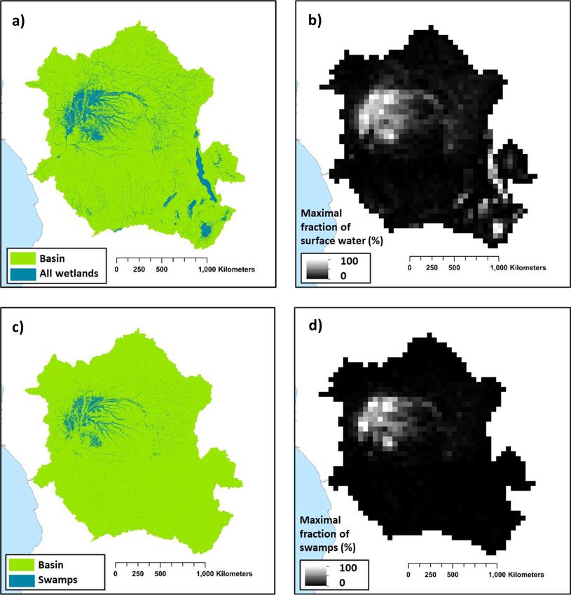
38                  A. Hastie et al.: Historical and future contributions of inland waters to the Congo Basin carbon balance

1    Introduction                                                  inland waters, or be transported to estuaries or the coast.
                                                                   The tropical region is a hotspot area for inland water C cy-
As the world’s second largest area of contiguous tropical          cling (Richey et al., 2002; Melack et al., 2004; Abril et al.,
rainforest and second largest river, the Congo Basin has a sig-    2014; Borges et al., 2015a; Lauerwald et al., 2015) due to
nificant role to play in the global carbon (C) cycle. Current      high terrestrial NPP and precipitation, and a recent study
estimates of its C stocks and fluxes are limited by a paucity      used an upscaling approach based on observations to esti-
of field data and therefore have substantial uncertainties, both   mate present-day CO2 evasion from the rivers of the Congo
quantified and unquantified (Williams et al., 2007; Lewis et       Basin at 251 ± 46 Tg C yr−1 and the lateral C (TOC + DIC)
al., 2009; Dargie et al., 2017). Nevertheless, it has been esti-   export to the coast at 15.5 (13–18) Tg C yr−1 (Borges at al.,
mated that there is approximately 50 Pg C stored in its above-     2015a, 2019). To put this into context, the estimate of aquatic
ground biomass (Verhegghen et al., 2012) and up to 100 Pg C        CO2 evasion represents 39 % of the global value estimated
contained within its soils (Williams et al., 2007). Moreover,      by Lauerwald et al. (2015, 650 Tg C yr−1 ) or 14 % of the
a recent study estimated that around 30 (6.3–46.8) Pg C is         global estimate of Raymond et al. (2013, 1800 Tg C yr−1 ).
stored in the peats of the Congo alone (Dargie at al., 2017).      Note that while Lauerwald et al. (2015) and Raymond et
Field data suggest that storage in tree biomass increased by       al. (2013) relied largely on the same database of partial pres-
0.34 (0.15–0.43) Pg C yr−1 in intact African tropical forests      sure of CO2 (pCO2 ) measurements (GloRiCh; Hartmann et
between 1968 and 2007 (Lewis et al., 2009) due in large            al., 2014) as the basis for their estimates, they took differ-
part to a combination of increasing atmospheric CO2 con-           ent, albeit both empirically led, approaches. Moreover, both
centrations and climate change (Ciais et al., 2009; Pan et         approaches were limited by a relative paucity of data from
al., 2015), while satellite data indicate that terrestrial net     the tropics, which also explains the high degree of uncer-
primary productivity (NPP) has increased by an average of          tainty associated with our understanding of global riverine
10 g C m−2 yr−1 per year between 2001 and 2013 in tropical         CO2 evasion.
Africa (Yin et al., 2017).                                            Whilst the importance of LOAC fluxes in the Congo Basin
   At the same time, forest degradation, clearing for rota-        has been demonstrated for the present day, it is not known
tional agriculture, and logging are causing C losses to the        to what extent these fluxes have been perturbed historically,
atmosphere (Zhuravleva et al., 2013; Tyukavina et al., 2018),      how they are likely to change under future climate change
while droughts have reduced vegetation greenness and water         and land use scenarios, and in turn what impact these changes
storage over the last decade (Zhou et al., 2014). A recent es-     might have on the overall C balance of the Congo. In light
timate of above-ground C stocks in tropical African forests,       of these knowledge gaps, we address the following research
mainly in the Congo, indicates a minor net C loss from 2010        questions.
to 2017 (Fan et al., 2019). Moreover, recent field data suggest
that the above-ground C sink in tropical Africa was relatively       – What is the relative contribution of LOAC fluxes (CO2
stable from 1985 to 2015 (Hubau et al., 2020).                         evasion and C export to the coast) to the present-day
   There are large uncertainties associated with projecting fu-        C balance of the basin?
ture trends in the Congo Basin terrestrial C cycle, firstly re-
                                                                     – To what extent have LOAC fluxes changed from 1861
lated to predicting which trajectories of future CO2 levels
                                                                       to the present day, and what are the primary drivers of
and land use changes will occur and secondly to our abil-
                                                                       this change?
ity to fully understand and simulate these changes and in
turn their impacts. Future model projections for the 21st cen-       – How will these fluxes change under future climate and
tury agree that temperature will significantly increase un-            land use change scenarios (RCP6.0, which represents
der both low and high emission scenarios (Haensler et al.,             the “no mitigation” scenario), and what are the limita-
2013), while precipitation is only projected to substantially          tions associated with these future projections?
increase under high emission scenarios, with the basin mean
remaining more or less unchanged under low emission sce-           Understanding and quantifying these long-term changes re-
narios (Haensler et al., 2013). Uncertainties in future land use   quires a complex and integrated mass-conservation mod-
change projections for Africa are among the highest for any        elling approach. The ORCHILEAK model (Lauerwald et al.,
continent (Hurtt et al., 2011).                                    2017), a new version of the land surface model ORCHIDEE
   For the present day at the global scale, it has been esti-      (Krinner et al., 2005), is capable of simulating observed ter-
mated that between 1 and 5 Pg C yr−1 is transferred later-         restrial and aquatic C fluxes in a consistent manner for the
ally to the land–ocean aquatic continuum (LOAC) as dis-            present day in the Amazon (Lauerwald et al., 2017) and Lena
solved CO2 , dissolved organic carbon (DOC), and particu-          (Bowring et al., 2019, 2020) basins, albeit with limitations
late organic carbon (POC) (Cole at al., 2007; Tranvik et al.,      including a lack of explicit representation of POC fluxes and
2009; Regnier et al., 2013; Drake et al., 2018; Ciais et al.,      in-stream autotrophic production (see Lauerwald et al., 2017;
2020). This C can subsequently be evaded back to the at-           Bowring et al., 2019, 2020; and Hastie et al., 2019, for fur-
mosphere as CO2 , undergo sedimentation in wetlands and            ther discussion). Moreover, it was recently demonstrated that

Earth Syst. Dynam., 12, 37–62, 2021                                                    https://doi.org/10.5194/esd-12-37-2021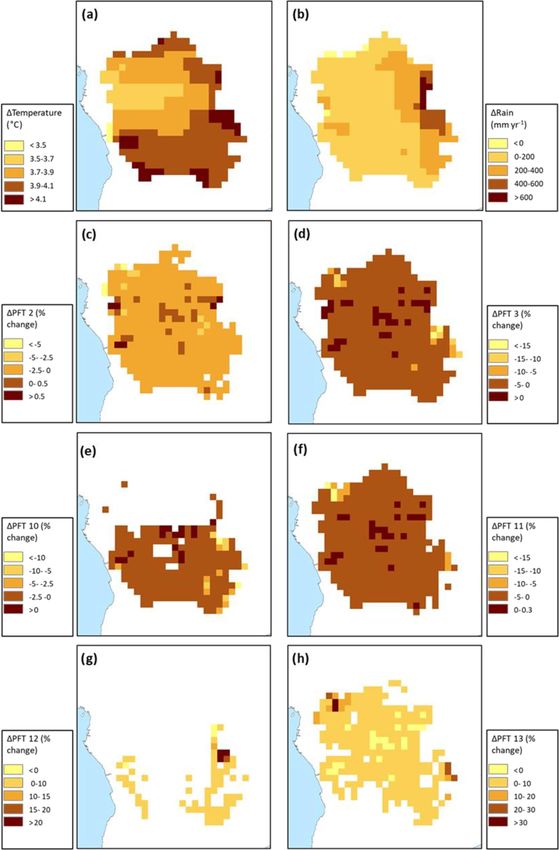
A. Hastie et al.: Historical and future contributions of inland waters to the Congo Basin carbon balance                              39

this model could recreate observed seasonal and interannual
variation in Amazon Basin aquatic and terrestrial C fluxes
(Hastie et al., 2019).
   In order to accurately simulate aquatic C fluxes, it is cru-
cial to provide a realistic representation of the hydrologi-
cal dynamics of the Congo River, including its wetlands.
Here, we develop new wetland forcing files for the OR-
CHILEAK model from the high-resolution dataset of Gum-
bricht et al. (2017) and apply the model to the Congo Basin.
After validating the model against observations of discharge,
flooded area, DOC concentrations, and pCO2 for the present
day, we then use the model to understand and quantify the
long-term (1861–2099) temporal trends in both the terrestrial
and aquatic C fluxes of the Congo Basin.

2   Methods
                                                                    Figure 1. Extent of the Congo Basin, central quadrant of the Cu-
ORCHILEAK (Lauerwald et al., 2017) is a branch of the OR-           vette Centrale, and locations of sampling stations used for validation
CHIDEE land surface model (LSM), building on past model             (of DOC, discharge, and partial pressure of CO2 ) along the Congo
developments such as ORCHIDEE-SOM (Camino-Serrano                   and Oubangui River (in italics).
et al., 2018), and represents one of the first LSM-based ap-
proaches which fully integrates the aquatic C cycle within the
terrestrial domain. ORCHILEAK simulates DOC production              resenting the maximal fraction of floodplains (MFF) and the
in the canopy and soils, the leaching of dissolved CO2 and          maximal fraction of swamps (MFS) (Sect. 2.2) and to recal-
DOC to the river from the soil, the mineralization of DOC,          ibrate the river-routing module of ORCHILEAK (Sect. 2.3).
and in turn the evasion of CO2 to the atmosphere from the           All of the processes represented in ORCHILEAK remain
water surface. Moreover, it represents the transfer of C be-        identical to those previously represented for the Amazon OR-
tween litter, soils, and water within floodplains and swamps        CHILEAK (Lauerwald et al., 2017; Hastie et al., 2019). In
(see Sect. 2.2). Once within the river-routing scheme, OR-          the following methodology sections, we describe the follow-
CHILEAK assumes that the lateral transfer of CO2 and DOC            ing: Sect. 2.1 – Congo Basin description; Sect. 2.2 – develop-
is proportional to the volume of water. DOC is divided into         ment of floodplain and swamp forcing files; Sect. 2.3 – cali-
a refractory and labile pool within the river, with half-lives      bration of hydrology; Sect. 2.4 – simulation set-up; Sect. 2.5
of 80 and 2 d, respectively. The refractory pool corresponds        – evaluation and analysis of simulated fluvial C fluxes; and
to the combined slow and passive DOC pools of the soil C            Sect. 2.6 – calculating the net carbon balance of the Congo
scheme, and the labile pool corresponds to the active soil          Basin. For a full description of the ORCHILEAK model,
pool (see Sect. 2.4.1). The concentration of dissolved CO2          please see Lauerwald et al. (2017).
and the temperature-dependent solubility of CO2 are used to
calculate pCO2 in the water column. In turn, CO2 evasion            2.1   Congo Basin description
is calculated based on pCO2 , along with a diurnally vari-
able water surface area and a gas exchange velocity. Fixed          The Congo Basin is the world’s second largest area of con-
gas exchange velocities of 3.5 and 0.65 m d−1 , respectively,       tiguous tropical rainforest and second largest river basin
are used for rivers (including open floodplains) and forested       (Fig. 1), covering an area of 3.7 × 10⁶ km2 , with a mean dis-
floodplains.                                                        charge of around 42 000 m−3 s−1 (O’Loughlin et al., 2013)
   In this study, as in previous studies (Lauerwald et al., 2017;   and a variation between 24 700 and 75 500 m−3 s−1 across
Hastie et al., 2019; Bowring et al., 2019, 2020), we run the        months (Coynel et al., 2005).
model at a spatial resolution of 1◦ and use the default time           The major climate (ISMSIP2b; Frieler et al., 2017; Lang
step of 30 min for all vertical transfers of water, energy, and     et al., 2017) and land cover (LUH-CMIP5) characteristics of
C between vegetation, soil, and the atmosphere, as well as          the Congo Basin for the present day (1981–2010) are shown
the daily time step for the lateral routing of water. Until         in Fig. 2. The mean annual temperature is 25.2 ◦ C but with
now, in the tropics, ORCHILEAK has been parameterized               considerable spatial variation from a low of 18.4 ◦ C to a high
and calibrated only for the Amazon River Basin (Lauerwald           of 27.2 ◦ C (Fig. 2a), while mean annual rainfall is 1520 mm,
et al., 2017; Hastie et al., 2019). To adapt and apply OR-          varying from 733 to 4087 mm (Fig. 2b). ORCHILEAK pre-
CHILEAK to the specific characteristics of the Congo River          scribes 13 different plant functional types (PFTs). Land use is
Basin (Sect. 2.1), we had to establish new forcing files rep-       mixed with tropical broadleaved evergreen (PFT2, Fig. 1c),

https://doi.org/10.5194/esd-12-37-2021                                                      Earth Syst. Dynam., 12, 37–62, 2021
40                  A. Hastie et al.: Historical and future contributions of inland waters to the Congo Basin carbon balance

Figure 2. Present-day (1981–2010) spatial distribution of the principal climate and land use drivers used in ORCHILEAK across the Congo
Basin; (a) mean annual temperature (◦ C), (b) mean annual rainfall (mm yr−1 ), (c–h) mean annual maximum vegetated fraction for PFTs 2,
3, 10, 11, 12, and 13, respectively; (i) river area; and (j) poor soils. All are at a resolution of 1◦ except for river area (0.5◦ ).

Earth Syst. Dynam., 12, 37–62, 2021                                                       https://doi.org/10.5194/esd-12-37-2021
A. Hastie et al.: Historical and future contributions of inland waters to the Congo Basin carbon balance                        41

tropical broadleaved rain green (PFT3, Fig. 1d), C3 grass          ing the “swamps” and “fens” wetland categories (although
(PFT10, Fig. 2e), and C4 grass (PFT11, Fig. 2f) covering a         note that there are virtually no fens in the Congo Basin) from
maximum of 26 %, 35 %, 8 %, and 25 % of the basin area,            the Global Wetlandsv3 database (Gumbricht et al., 2017) and
respectively. Most published estimates for land cover fol-         again aggregating them to a 0.5◦ resolution. Please see Ta-
low national boundaries, so we can make broad compar-              ble 1 of Gumbricht et al. (2017) for further details.
isons with published estimates for the Democratic Repub-
lic of Congo (DRC). For example, our value for total forest        2.3   Calibration of hydrology
cover for the DRC (65 %) is close to the 67 % and 68 % val-
ues estimated by the Congo Basin Forest Partnership (CBFP,         As the main driver of the export of C from the terrestrial to
2009) and Potapov et al. (2012), respectively. Agriculture         the aquatic system, it is crucial that the model can represent
covers only a small proportion of the basin according to the       present-day hydrological dynamics, at the very least on the
LUH dataset that is based on FAO cropland area statistics,         main stem of the Congo. As this study is primarily concerned
with C3 (PFT12, Fig. 2g) and C4 (PFT13, Fig. 2h) agricul-          with decadal to centennial timescales our priority was to en-
ture making up a maximum basin area of 0.5 % and 2 %, re-          sure that the model can accurately recreate observed mean
spectively. In reality, a larger fraction of the basin is com-     annual discharge at the most downstream gauging station at
posed of small-scale and rotational agriculture (Tyukavina et      Brazzaville. We also tested the model’s ability to simulate
al., 2018). The ORCHILEAK model also has a “poor soils”            observed discharge seasonality and flood dynamics. More-
forcing file (Fig. 2j) which prescribes reduced decomposi-         over, no data are available with which to directly evaluate
tion rates in soils with low-nutrient and low-pH soils such        the simulation of DOC and CO2 leaching from the soil to the
as Podzols and Arenosols (Lauerwald et al., 2017). This            river network, and thus we tested the model’s ability to recre-
file is developed from the Harmonized World Soil Database          ate the spatial variation of observed riverine DOC concentra-
(FAO/IIASA/ISRIC/ISS-CAS/JRC, 2009).                               tions and pCO2 at specific stations where measurements are
                                                                   available (Borges at al., 2015b; Bouillon et al., 2012, 2014;
2.2   Development of floodplain and swamp forcing files
                                                                   locations shown in Fig. 1), with the river DOC and CO2 con-
                                                                   centration being regarded as an integrator of the C transport
In ORCHILEAK, water in the river network can be diverted           at the terrestrial–aquatic interface.
to two types of wetlands: floodplains and swamps. In each             We first ran the model for the present-day period, defined
grid wherein a floodplain exists, a temporary water body           as 1990 to 2005–2010 depending on which climate forc-
can be formed adjacent to the river and is fed by the river        ing data were applied, using four climate forcing datasets,
once bankfull discharge (see Sect. 2.3) is exceeded. In grids      namely ISIMIP2b (Frieler et al., 2017), Princeton GPCC
wherein swamps exist, a constant proportion of river dis-          (Sheffield et al., 2006), GSWP3 (Kim, 2017), and CRUN-
charge is fed into the base of the soil column; ORCHILEAK          CEP (Viovy, 2018). We used ISIMIP2b for the historical and
does not explicitly represent a groundwater reservoir, so this     future simulations as it is the only climate forcing dataset
imitates the hydrological coupling of swamps and rivers            to cover the full period (1861–2099). However, we com-
through the groundwater table. The maximal proportions of          pared it to other climate forcing datasets for the present
each grid which can be covered by floodplains and swamps           day in order to gauge its ability to simulate observed dis-
are prescribed by the maximal fraction of floodplain (MFF)         charge on the Congo River at Brazzaville (Table A1). With-
and the maximal fraction of swamp (MFS) forcing files, re-         out calibration, the majority of the different climate forc-
spectively (Guimberteau et al., 2012). See also Lauerwald et       ing model runs performed poorly and were unable to accu-
al. (2017) and Hastie et al. (2019) for further details. We cre-   rately represent the seasonality and mean monthly discharge
ated an MFF forcing file for the Congo Basin derived from          at Brazzaville (Table A1). The best-performing climate forc-
the Global Wetlandsv3 database, which includes the 232 m           ing dataset was ISIMIP2b, followed by Princeton GPCC,
resolution tropical wetland map of Gumbricht et al. (2017)         with root mean square errors (RMSEs) of 29 % and 40 %
(Fig. 3a and b). We firstly amalgamated all the categories         and a Nash–Sutcliffe efficiency (NSE) of 0.20 and −0.25,
of wetland (which include floodplains and swamps) before           respectively. NSE is a statistical coefficient specifically used
aggregating them to a resolution of 0.5◦ (the resolution at        to test the predictive skill of hydrological models (Nash and
which the floodplain and swamp forcing files are read by           Sutcliffe, 1970).
ORCHILEAK), assuming that this represents the maximum                 For ISIMIP2b we further calibrated key hydrological
extent of inundation in the basin. This results in a mean          model parameters, namely the constants (tau, τ ) which help
MFF of 10 %; i.e. a maximum of 10 % of the surface area            to control the water residence time of the groundwater (slow
of the Congo Basin can be inundated with water. This is            reservoir), headwaters (fast reservoir), and floodplain reser-
identical to the mean MFF value of 10 % produced with the          voirs in order to improve the simulation of observed dis-
Global Lakes and Wetlands Database, GLWD (Lehner and               charge at Brazzaville and Oubangui (Table 2). To do so, we
Döll, 2004; Borges et al., 2015b). We also created an MFS          tested different combinations of τ values for the three reser-
forcing file from the same dataset (Fig. 3c and d), merg-          voirs, eventually settling on 1, 0.5, and 0.5 (d) for the slow,

https://doi.org/10.5194/esd-12-37-2021                                                   Earth Syst. Dynam., 12, 37–62, 2021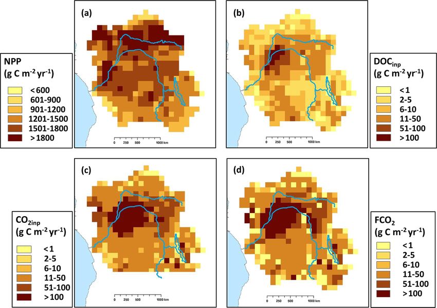
42                  A. Hastie et al.: Historical and future contributions of inland waters to the Congo Basin carbon balance

Figure 3. (a) Wetland extent (from Gumbricht et al., 2017). (b) The new maximal fraction of floodplain (MFF) forcing file developed
from (a). (c) The swamp (including fens) category within the Congo Basin from Gumbricht et al. (2017). (d) The new maximal fraction of
swamp (MFS) forcing file developed from (c). Panels (a) and (b) are at the same resolution as the Gumbricht dataset (232 m), while panels
(b) and (d) are at a resolution of 0.5◦ . Note that 0.5◦ is the resolution of the subunit basins in ORCHILEAK (Lauerwald et al., 2015), with
each 1◦ grid containing four sub-basins.

fast, and floodplain reservoirs, respectively, with all three be-       forcing period (1990 to 2005). After re-running each model
ing reduced compared to those values used in the original               parametrization (different τ values) to obtain those bankfull
ORCHILEAK calibration for the Amazon (Lauerwald at al.,                 discharge values, we calculated floodh95th over the simula-
2017). The actual residence time of each reservoir is calcu-            tion period for each grid cell (Table 1). This value is assumed
lated at each time step. The residence time of the flooded              to represent the water level over the riverbanks at which
reservoir, for example, is a product of τflood , a topographical        the maximum horizontal extent of floodplain inundation is
index, and the flooded fraction of the grid cell.                       reached. We then ran the model for a final time and validated
   In order to calibrate the simulated discharge against ob-            the outputs against discharge data at Brazzaville (Cochon-
servations, we first modified the flood dynamics of OR-                 neau et al., 2006; Fig. 1). This procedure was repeated itera-
CHILEAK in the Congo Basin for the present day by adjust-               tively with the ISIMIP2b climate forcing with modifying the
ing bankfull discharge (streamr50th ; Lauerwald et al., 2017)           τ value of each reservoir in order to find the best-performing
and the 95th percentile of water level heights (floodh95th ).           parametrization.
As in previous studies on the Amazon Basin (Lauerwald et                   We firstly compared simulated versus observed discharge
al., 2017; Hastie et al., 2019) we defined bankfull discharge,          at Brazzaville (NSE, RMSE; Table 2), before using the data
i.e. the threshold discharge at which floodplain inundation             of Bouillon et al. (2014) to further validate discharge at Ban-
starts (i.e. overtopping of banks), as the median discharge             gui (Fig. 1) on the main tributary Oubangui. In addition, we
(50th percentile i.e. streamr50th ) of the present-day climate          compared the simulated seasonality of flooded area against

Earth Syst. Dynam., 12, 37–62, 2021                                                           https://doi.org/10.5194/esd-12-37-2021
A. Hastie et al.: Historical and future contributions of inland waters to the Congo Basin carbon balance                                 43

Table 1. Main forcing files used for simulations.

                   Variable                                       Spatial     Temporal      Data source
                                                               resolution     resolution
                   Rainfall, incoming shortwave and                   1◦      1d            ISIMIP2b, IPSL-CM5A-LR
                   longwave radiation, air temperature,                                     model outputs for RCP6.0
                   relative humidity and air pressure                                       (Frieler et al., 2017)
                   (close to the surface), wind speed (10 m
                   above the surface)
                   Land cover (and change)                           0.5◦     annual        LUH-CMIP5
                   Poor soils                                        0.5◦     annual        Derived from HWSD v 1.1
                                                                                            (FAO/IIASA/ISRIC/ISS-
                                                                                            CAS/JRC, 2009)
                   Streamflow directions                             0.5◦     annual        STN-30p (Vörösmarty et al.,
                                                                                            2000)
                   Floodplain and swamp fraction in                  0.5◦     annual        Derived from the wetland high-
                   each grid (MFF and MFS)                                                  resolution data of Gumbricht et
                                                                                            al. (2017)
                   River surface areas                               0.5◦     annual        Lauerwald et al. (2015)
                   Bankfull discharge (streamr50th )                  1◦      annual        Derived from calibration with
                                                                                            ORCHILEAK (see Sect. 2.3)
                   95th percentile of water table height              1◦      annual        Derived from calibration with
                   over floodplain (floodh95th )                                            ORCHILEAK (see Sect. 2.3)

Table 2. Performance statistics for the modelled versus observed seasonality of discharge at Brazzaville and Bangui, as well as flooded area
in Cuvette Centrale. Observed flooded area is from GIEMS (Papa et al., 2010; Becker et al., 2018).

                          Station        RMSE          NSE    R2        Simulated mean              Observed mean
                                                                       monthly discharge          monthly discharge
                                                                               (m3 s−1 )                  (m3 s−1 )
                          Brazzaville      23 %        0.66   0.84                     38 944                 40 080
                          Bangui           59 %        0.31   0.88                      1448                   2923
                                                                         Simulated mean             Observed mean
                                                                     monthly flooded area       monthly flooded area
                                                                                (103 km2 )                 (103 km2 )
                          Flooded
                          area
                                         272 %      −1.44     0.67                         44                     14
                          (Cuvette
                          Centrale)

the satellite-derived dataset GIEMS (Prigent et al., 2007;                  and the 95th percentile of water table height over flood-
Becker et al., 2018) within the Cuvette Centrale wetlands                   plain (floodh95th ) (Table 1) is described in Sect. 2.3.
(Fig. 1).
                                                                            2.4.1   Soil carbon spin-up
2.4   Simulation set-up
                                                                            ORCHILEAK includes a soil module, primarily derived
A list of the main forcing files used, along with data sources,             from ORCHIDEE-SOM (Camino-Serrano et al., 2018). The
is presented in Table 1. The derivation of the floodplains                  soil module has three different pools of soil DOC: the pas-
and swamps (MFF and MFS) is described in Sect. 2.2,                         sive, slow, and active pool, and these are defined by their
while the calculation of bankfull discharge (streamr50th )                  source material and residence times (τcarbon ). ORCHILEAK

https://doi.org/10.5194/esd-12-37-2021                                                             Earth Syst. Dynam., 12, 37–62, 2021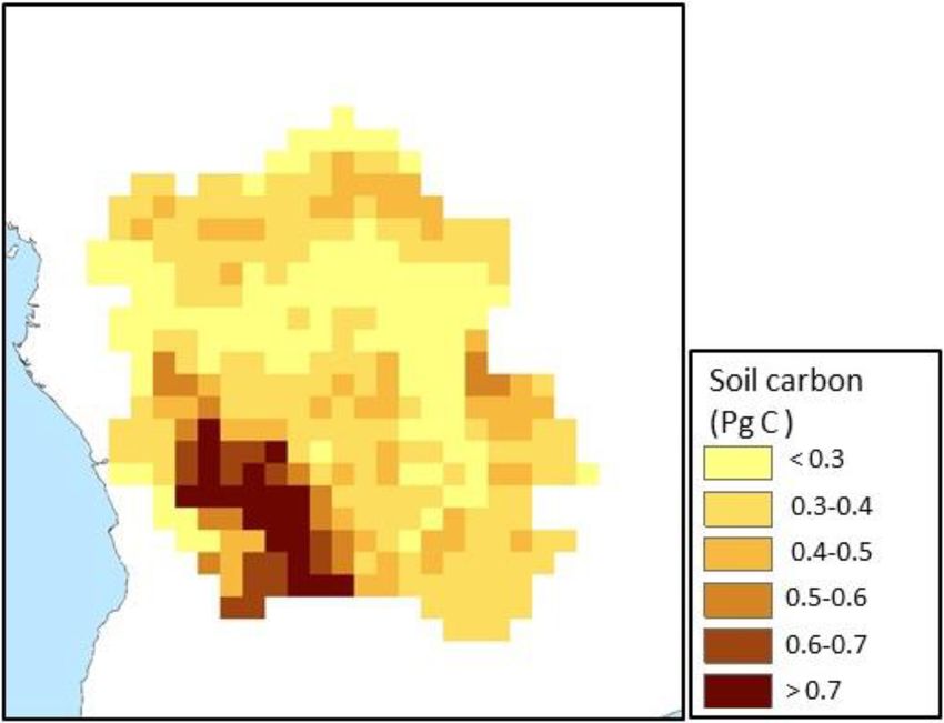
44                 A. Hastie et al.: Historical and future contributions of inland waters to the Congo Basin carbon balance

also differentiates between flooded and non-flooded soils          the ISIMIP2b data only provided two Representative Con-
as well as the decomposition rates of DOC, soil organic            centration Pathways (RCPs) at the time we performed the
carbon (SOC), and litter being reduced (3 times lower) in          simulations: RCP2.6 (low emission) and RCP6.0.
flooded soils. In order for the soil C pools to reach steady          With the purpose of separately evaluating the effects of
state, we spun up the model for around 9000 years with fixed       land use change, climate change, and rising atmospheric
land use representative of 1861 and looping over the first         CO2 , we ran a series of factorial simulations. In each sim-
30 years of the ISMSIP2b climate forcing data (1861–1890).         ulation, one of these factors was fixed at its 1861 level (the
During the first 2000 years of spin-up, we ran the model with      first year of the simulation), or in the case of fixed climate
an atmospheric CO2 concentration of 350 µ atm and default          change, we looped over the years 1861–1890. The outputs
soil C residence times (τcarbon ) halved, which allowed it to      of these simulations (also 30-year running means) were then
approach steady state more rapidly. Following this, we ran         subtracted from the outputs of the main simulation (original
the model for a further 7000 years, reverting to the default       run with all factors varied) so that we could determine the
τcarbon values. At the end of this process, the soil C pools had   contribution of each driver (Fig. 11, Table 1).
reached approximately steady state, with < 0.02 % change in
each pool over the final century of the spin-up.                   2.5   Evaluation and analysis of simulated fluvial C fluxes
                                                                   We first evaluated DOC concentrations and pCO2 at several
2.4.2   Transient simulations                                      locations along the Congo main stem (Fig. 1) and on the
After the spin-up, we ran a historical simulation from 1861        Oubangui River against the data of Borges at al. (2015b) and
until the present day, which is 2005 in the case of the            Bouillon et al. (2012, 2014). We also compared the various
ISIMIP2b climate forcing data. We then ran a future simu-          simulated components of the net C balance (e.g. NPP) of the
lation until 2099 using the final year of the historical sim-      Congo against values described in the literature (Williams et
ulation as a restart file. In both of these simulations, cli-      al., 2007; Lewis et al., 2009; Verhegghen et al., 2012; Valen-
mate, atmospheric CO2 , and land cover change were pre-            tini et al., 2014; Yin et al., 2017). In addition, we assessed
scribed as fully transient forcings according to the RCP6.0        the relationship between the interannual variation in present-
scenario. For climate variables, we used the IPSL-CM5A-LR          day (1981–2010) C fluxes of the Congo Basin and variation
model outputs for RCP6.0 bias-corrected by the ISIMIP2b            in temperature and rainfall. This was done through linear re-
procedure (Frieler et al., 2017; Lange, 2017), while land use      gression using STATISTICATM . We found trends in several
change was taken from the 5th Coupled Model Intercom-              of the fluxes over the 30-year period (1981–2010) and thus
parison Project (CMIP5). As our aim is to investigate long-        detrended the time series with the “Detrend” function, part of
term trends, we calculated 30-year running means of simu-          the “SpecsVerification” package in R (R Core Team, 2013),
lated C flux outputs in order to smooth interannual variations.    before undertaking the statistical analysis focused on the cli-
RCP6.0 is an emissions pathway that leads to a stabilization       mate drivers of interannual variability.
of radiative forcing at 6.0 watts per square metre (W m−2 )
in the year 2100 without exceeding that value in prior years       2.6   Calculating the net carbon balance of the Congo
(Masui et al., 2011). It is characterized by intermediate en-            Basin
ergy intensity, substantial population growth, middle to high
                                                                   We calculated net ecosystem production (NEP) by sum-
C emissions, increasing cropland area to 2100, and decreas-
                                                                   ming the terrestrial and aquatic C fluxes of the Congo Basin
ing natural grassland area (van Vuuren et al., 2011). In the
                                                                   (Eq. 1), while we incorporated disturbance fluxes (land use
paper which describes the development of the future land
                                                                   change flux and harvest flux) to calculate net biome produc-
use change scenarios under RCP6.0 (Hurtt et al., 2011), it
                                                                   tion (NBP) (Eq. 2). Positive values of NBP and NEP equate
is shown that land use change is highly sensitive to land use
                                                                   to a net terrestrial C sink.
model assumptions, such as whether or not shifting cultiva-
                                                                      NEP is defined as follows:
tion is included. The LUH1 reconstruction, for instance, in-
dicates shifting cultivation affecting all of the tropics with a   NEP = NPP + TF − SHR − FCO2 − LEAquatic ,                  (1)
residence time of agriculture of 15 years, whereas the review
from Heinimann et al. (2017) revised the area of this type         where NPP is terrestrial net primary production, TF is the
of agriculture downwards, with generally low values in the         throughfall flux of DOC from the canopy to the ground,
Congo except in the northeast and southeast, but suggested         SHR is soil heterotrophic respiration (only that evading from
a shorter turnover of agriculture of only 2 years. In view of      the terra firme soil surface), FCO2 is CO2 evasion from the
such uncertainties, we did not include shifting agriculture in     water surface, and LEAquatic is the lateral export flux of C
the model. Moreover, there is considerable uncertainty as-         (DOC + dissolved CO2 ) to the coast. NBP is equal to NEP
sociated with the effect of future land use change in Africa       except with the inclusion of the C lost (or possibly gained)
(Hurtt et al., 2011). We chose RCP6.0 as it represents a no        via land use change (LUC) and crop harvest (HAR). Wood
mitigation (middle to high emissions) scenario. Moreover,          harvest is not included for logging and forestry practices, but

Earth Syst. Dynam., 12, 37–62, 2021                                                    https://doi.org/10.5194/esd-12-37-2021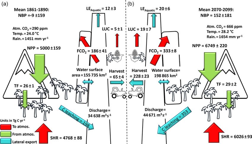
A. Hastie et al.: Historical and future contributions of inland waters to the Congo Basin carbon balance 45
during deforestation LUC, a fraction of the forest biomass
is harvested and channelled to wood product pools with dif-
ferent decay constants. LUC includes land conversion fluxes
and the lateral export of wood product biomass, assuming
that wood products from deforestation are not consumed and
released as CO2 over the Congo but in other regions:
NBP = NEP − (LUC + HAR). (2)
3 Results
3.1 Simulation of hydrology and aquatic carbon fluxes
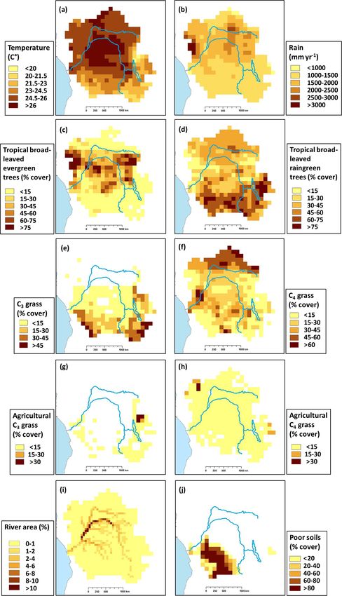
The final model configuration is able to closely reproduce the
mean monthly discharge at Brazzaville (Fig. 4a, Table 2) and
captures the seasonality moderately well (Fig. 4a, Table 2;
RMSE = 23 %, R 2 = 0.84 versus RMSE = 29 %, R 2 = 0.23
without calibration; Table A1). At Bangui on the Oubangui
River (Fig. 1), the model is able to closely recreate observed
seasonality (Fig. 4b; RMSE = 59 %, R 2 = 0.88) but substan-
tially underestimates the mean monthly discharge, with our
value being only 50 % of the observed. We produce reason-
able NSE values of 0.66 and 0.31 for Brazzaville and Bangui,
respectively, indicating that the model is moderately accurate
in its simulation of seasonality.
We also evaluated the simulated seasonal change in
flooded area in the central (approx. 200 000 km2 ; Fig. 1) part
of the Cuvette Centrale wetlands against the GIEMS inunda-
tion dataset (1993–2007, maximum inundation minus mini-
mum or permanent water bodies; Prigent et al., 2007; Becker
et al., 2018). While our model is able to represent the sea-
sonality in flooded area relatively well (R 2 = 0.75; Fig. 4c),
it considerably overestimates the magnitude of flooded area
relative to GIEMS (Fig. 4c, Table 2). However, the dataset
Figure 4. Seasonality of simulated versus observed discharge at
that we used to define the MFF and MFS forcing files (Gum- (a) Brazzaville on the Congo (for the 1990–2005 monthly mean;
bricht et al., 2017) is produced at a higher resolution than Cochonneau et al., 2006), (b) Bangui on the Oubangui (2010–
GIEMS and will capture smaller wetlands than the GIEMS 2012; Bouillon et al., 2014), and (c) flooded area in the central
dataset; thus, the greater flooded area is to be expected. (approx. 200 000 km2 ) part of the Cuvette Centrale wetlands ver-
GIEMS is also known to underestimate inundation under sus GIEMS (1993–2007; Becker et al., 2018). The observed flooded
vegetated areas (Prigent et al., 2007; Papa et al., 2010) and area data represent the maximum minus minimum (permanent wa-
has difficulties capturing small inundated areas (Prigent et ter bodies such as rivers) GIEMS inundation. See Fig. 1 for loca-
al., 2007; Lauerwald et al., 2017). Indeed, with the GIEMS tions.
data we produce an overall flooded area for the Congo Basin
of just 3 %, less than one-third of that produced with the
Gumbricht dataset (Gumbricht et al., 2017) or the GLWD able to simulate the broad spatial pattern of pCO2 measured
(Lehner and Döll, 2004). As such, it is to be expected that in the main-stem Congo reported by Borges et al. (2019).
there is a large RMSE (272 %; Table 2) between simulated During the high-flow season (2009–2019 mean of 6 con-
flooded area and GIEMS; more importantly, the seasonality secutive months of highest flow to account for interannual
of the two is highly correlated (R 2 = 0.67; Table 2). variation) we simulate a mean pCO2 of 3373 and 5095 ppm
In Fig. 5, we compare simulated DOC concentrations at at Kisangani and Kinshasa (Brazzaville), respectively, com-
six locations (Fig. 1) along the Congo River and Oubangui pared to the observed values of 2424 and 5343 ppm during
tributary against the observations of Borges at al. (2015b). high water (measured in December 2013; Borges et al., 2019)
We show that we can recreate the spatial variation in the DOC (Table 3). Similarly, during the low-flow season (mean of
concentration within the Congo Basin relatively closely with 6 consecutive months of lowest flow, 2009–2019) we sim-
an R 2 of 0.74 and an RMSE of 24 % (Fig. 5). We are also ulate a mean pCO2 of 1563 and 2782 ppm at Kisangani and
https://doi.org/10.5194/esd-12-37-2021 Earth Syst. Dynam., 12, 37–62, 2021
46 A. Hastie et al.: Historical and future contributions of inland waters to the Congo Basin carbon balance
Figure 5. Observed (Borges et al., 2015a) versus simulated DOC
concentrations at several sites along the Congo and Oubangui rivers. Figure 6. Time series of observed versus simulated pCO2 at Ban-
See Fig. 1 for locations. The simulated and observed DOC concen- gui on the River Oubangui. Observed data are from Bouillon et
trations represent the median values across the particular sampling al. (2012, 2014).
period at each location detailed in Borges et al. (2015a).
Kinshasa, respectively, compared to the observed values of
1670 and 2896 ppm during falling water (June 2014; Borges
et al., 2019) (Table 3).
While we are able to recreate observed spatial differences
in DOC and pCO2 , as well as broad seasonal variations, we
are not able to correctly predict the exact timing of the sim-
ulated highs and lows, a reflection of not fully capturing the
hydrological seasonality. For example, our mean June pCO2
at Kinshasa (Brazzaville) is 4470 ppm, while Borges et al.
measured a mean of 2896 ppm (Table 3). However, our value
for July of 2621 ppm is much closer, and moreover our mean
value for December of 5154 ppm is relatively close to the ob-
served value of 5343 ppm. Similarly, we fail to predict the
timing of the June falling water at Kisangani (Table 3).
In Fig. 6, we compare simulated pCO2 against the ob-
served monthly time series at Bangui on the Oubangui River
(Bouillon et al., 2012, 2014), which as far as we are aware is
the longest time series of pCO2 published (and accessible)
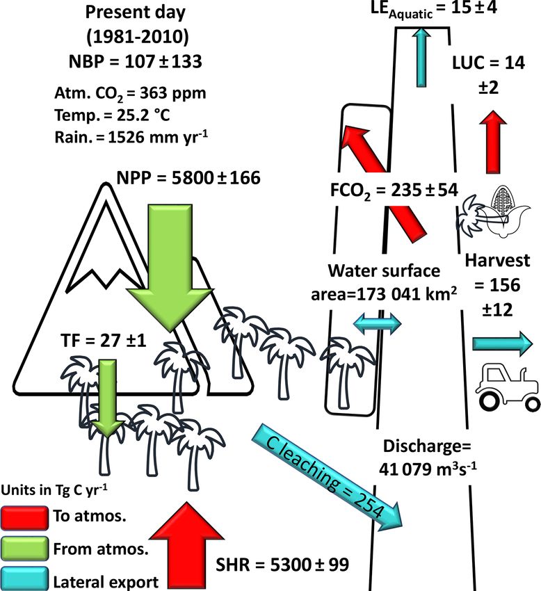
Figure 7. Annual C budget (NBP, net biome production) for
from the Congo Basin, spanning March 2010 to March 2012
the Congo Basin for the present day (1981–2010) simulated with
(with only the single month of June 2010 missing). Again, ORCHILEAK; NPP is terrestrial net primary productivity, TF is
while the model fails to correctly predict the precise timing throughfall, SHR is soil heterotrophic respiration, FCO2 is aquatic
of the peak as with the Kinshasa and Kisangani datasets, the CO2 evasion, C leaching is C leakage to the land–ocean aquatic
broad seasonal variation in pCO2 is captured, with the ob- continuum (FCO2 + LEAquatic ), LUC is the flux from land use
served and modelled times series ranging from 227–4040 and change, and LEAquatic is the export C flux to the coast. Range rep-
415–2928 ppm, respectively (Fig. 6). resents the standard deviation (SD) from 1981–2010.
3.2 Carbon fluxes along the Congo Basin for the
present day rainfall (detrended R 2 = 0.41, p < 0.001; Table A2) and a
negative correlation between annual NPP and temperature
For the present day (1981–2010) we estimate a mean an- (detrended R 2 = 0.32, p < 0.01; Table A2). We also see con-
nual terrestrial net primary production (NPP) of 5800 ± siderable spatial variation in NPP across the Congo Basin
166 Tg C yr−1 (standard deviation, SD) (Fig. 7), correspond- (Fig. 8a).
ing to a mean areal C fixation rate of approximately We simulate a mean soil heterotrophic respiration (SHR)
1500 g C m−2 yr−1 (Fig. 8a). We find a significant positive of 5300±99 Tg C yr−1 across the Congo Basin (Fig. 7). Con-
correlation between the interannual variation of NPP and trary to NPP, interannual variation in annual SHR is pos-
Earth Syst. Dynam., 12, 37–62, 2021 https://doi.org/10.5194/esd-12-37-2021A. Hastie et al.: Historical and future contributions of inland waters to the Congo Basin carbon balance 47
Table 3. Observed (Borges et al., 2019) and modelled pCO2 (in ppm) at Kinshasa (Brazzaville) and Kisangani on the Congo River at various
water levels.
Location Observed Modelled Modelled Observed Modelled Modelled
pCO2 pCO2 pCO2 pCO2 pCO2 pCO2
high water high water high-flow season falling falling low-flow season
(December (December (mean of 6 water water (mean of 6
2013) Mean consecutive (June (June consecutive
2009–2019) months of highest 2014) mean months of
flow 2009–2019) 2009–2019) lowest flow
2009–2019)
Kinshasa (Brazzaville) 5343 5154 5095 2896 4470 2782
Kisangani 2424 2166 3373 1670 3126 1563
Figure 8. Present-day (1981–2010) spatial distribution of (a) terrestrial net primary productivity (NPP), (b) dissolved organic carbon export
from soils and floodplain vegetation into the aquatic system (DOCinp ), (c) CO2 leaching from soils and floodplain vegetation into the aquatic
system (CO2inp ), and (d) aquatic CO2 evasion (FCO2 ). Main rivers are in blue. All are at a resolution of 1◦ .
itively correlated with temperature (detrended R 2 = 0.57, restrial DOC leaching (DOCinp ) (R 2 = 0.81, p < 0.0001;
p < 0.0001; Table A2) and inversely correlated with rain- Fig. 8b) and terrestrial CO2 leaching (CO2inp ) (R 2 = 0.96,
fall (detrended R 2 = 0.10), though the latter relationship p < 0.0001, Fig. 8c) into the aquatic system, but not ter-
is not significant (p > 0.05). We estimate a mean annual restrial NPP (R 2 = 0.01, p < 0.05; Fig. 8a). We simulate a
aquatic CO2 evasion rate of 1363±83 g C m−2 yr−1 , amount- mean annual flux of DOC throughfall from the canopy of
ing to a total of 235 ± 54 Tg C yr−1 across the total water 27 ± 1 Tg C yr−1 and C (DOC + dissolved CO2 ) export flux
surfaces of the Congo Basin (Fig. 7), and attribute 85 % of to the coast of 15 ± 4 Tg C yr−1 (Fig. 7).
this flux to flooded areas, meaning that only 32 Tg C yr−1 For the present day (1981–2010) we estimate a mean an-
is evaded directly from the river surface. Interannual vari- nual net ecosystem production (NEP) of 277±137 Tg C yr−1
ation in aquatic CO2 evasion (1981–2010) shows a strong and a net biome production (NBP) of 107 ± 133 Tg C yr−1
positive correlation with rainfall (detrended R 2 = 0.75, p < (Fig. 7). Interannually, both NEP and NBP exhibit a strong
0.0001; Table A2) and a weak negative correlation with tem- inverse correlation with temperature (detrended NEP R 2 =
perature (detrended R 2 = 0.09, not significant, p > 0.05). 0.55, p < 0.0001, detrended NBP R 2 = 0.54, p < 0.0001)
Aquatic CO2 evasion also exhibits substantial spatial vari- and weak positive relationship with rainfall (detrended NEP
ation (Fig. 8d), displaying a pattern similar to both ter- R 2 = 0.16, p < 0.05, detrended NBP R 2 = 0.14, p < 0.05).
https://doi.org/10.5194/esd-12-37-2021 Earth Syst. Dynam., 12, 37–62, 202148 A. Hastie et al.: Historical and future contributions of inland waters to the Congo Basin carbon balance
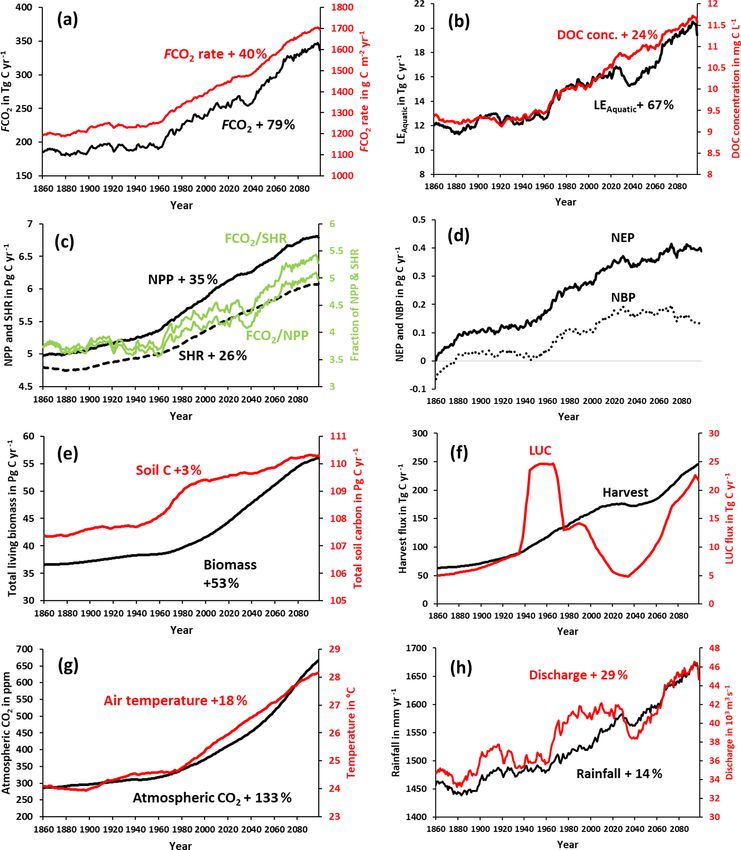
Figure 9. Simulation results for various C fluxes and stocks from 1861–2099 using IPSL-CM5A-LR model outputs for RCP6.0 (Frieler et
al., 2017). All panels except for atmospheric CO2 , biomass, and soil C correspond to 30-year running means of simulation outputs. This was
done in order to suppress interannual variation, as we are interested in longer-term trends.
Furthermore, we simulate a present-day (1981–2010) living the increase until the present day (1981–2010 mean) is
biomass of 41±1 Pg C and a total soil C stock of 109±1 Pg C. +26 % (to 235 Tg C yr−1 ), though these trends are not uni-
form across the basin (Fig. A1). The lateral export flux
of C to the coast (LEAquatic ) follows a similar relative
3.3 Long-term temporal trends in carbon fluxes change (Fig. 9b), rising by 67 % in total from 12 Tg C yr−1
We find an increasing trend in aquatic CO2 evasion (Fig. 9a) (Fig. 10) to 15 Tg C yr−1 for the present day and finally to
throughout the simulation period, rising slowly at first until 20 Tg C yr−1 (2070–2099 mean; Fig. 10). This is greater than
the 1960s when the rate of increase accelerates. In total CO2 the equivalent increase in DOC concentration (24 %; Fig. 9b)
evasion rose by 79 % from 186 Tg C yr−1 at the start of the due to the concurrent rise in rainfall (by 14 %; Fig. 9h) and
simulation (1861–1890 mean) (Fig. 10) to 333 Tg C yr−1 at in turn discharge (by 29 %; Fig. 9h).
the end of this century (2070–2099 mean; Fig. 10), while
Earth Syst. Dynam., 12, 37–62, 2021 https://doi.org/10.5194/esd-12-37-2021A. Hastie et al.: Historical and future contributions of inland waters to the Congo Basin carbon balance 49
Figure 10. Annual C budget (NBP, net biome production) for the Congo Basin for (a) 1861–1890 and (b) 2070–2099, simulated with
ORCHILEAK; NPP is terrestrial net primary productivity, TF is throughfall, SHR is soil heterotrophic respiration, FCO2 is aquatic CO2
evasion, C leaching is C leakage to the land–ocean aquatic continuum (FCO2 + LEAquatic ), LUC is the flux from land use change, and
LEAquatic is the export C flux to the coast. Range represents the standard deviation (SD).
Terrestrial NPP and SHR also exhibit substantial increases across the simulation period (Fig. 11). They are responsible
of 35 % and 26 %, respectively, across the simulation pe- for the vast majority of the growth in NPP, SHR, aquatic
riod and similarly rise rapidly after 1960 (Fig. 9c). NEP, CO2 evasion, and the flux of C to the coast (Fig. 11a–d).
NBP (Fig. 9d), and living biomass (Fig. 9e) follow roughly The effect of LUC on these four fluxes is more or less neu-
the same trend as NPP, but NEP and NBP begin to slow tral, while the impact of climate change is more varied. The
down or even level off around 2030, and in the case of aquatic fluxes (Fig. 11c and d) respond positively to an accel-
NBP, we actually simulate a decreasing trend over approx- eration in the increase of both rainfall (and in turn discharge;
imately the final 50 years. Interestingly, the proportion of Fig. 9h) and temperature (Fig. 9g) starting around 1970.
NPP lost to the LOAC also increases from approximately 3 % From around 2020, the impact of climate change on the lat-
to 5 % (Fig. 9c). We also find that living biomass stock in- eral flux of C to the coast (Fig. 11d) reverts to being effec-
creases by a total of 53 % from 1861 to 2099. Total soil C tively neutral, likely a response to a slowdown in the rise
also increases over the simulation but only by 3 % from of rainfall and indeed a decrease in discharge (Fig. 9h), as
107 to 110 Pg C yr−1 (Fig. 9e). Emissions from land use well as perhaps the effect of temperature crossing a thresh-
change (LUC) show considerable decadal fluctuation, in- old. The response of the overall loss of terrestrial C to the
creasing rapidly in the second half of the 20th century and LOAC (i.e. the ratio of LOAC to NPP; Fig. 11e) is relatively
decreasing in the mid-21st century before rising again to- similar to the response of the individual aquatic fluxes, but
wards the end of the simulation (Fig. 9f). The harvest flux crucially, climate change exerts a much greater impact, con-
(Fig. 9f) rises throughout the simulation with the exception tributing substantially to an increase in the loss of terrestrial
of a period in the mid-21st century during which it stalls for NPP to the LOAC in the 1960s and again in the second half
several decades. This is reflected in the change in land use of the 21st century. These changes closely coincide with the
areas from 1861–2099 (Fig. A2) during which the natural pattern of rainfall and in particular with changes in discharge
forest and grassland PFTs marginally decrease, while both (Fig. 9h).
C3 and C4 agricultural grassland PFTs increase. Overall temperature and rainfall increase by 18 % and
14 % from 24 to 28 ◦ C and 1457 to 1654 mm, respectively,
but in Fig. A2 one can see that this increase is non-uniform
3.4 Drivers of simulated trends in carbon fluxes across the basin. Generally speaking, the greatest increase in
The dramatic increase in the concentration of atmospheric temperature occurs in the south of the basin, while it is the
CO2 (Fig. 9g) and subsequent fertilization effect on terres- east that sees the largest rise in rainfall (Fig. A2). Land use
trial NPP have the greatest overall impact on all of the fluxes changes are similarly non-uniform (Fig. A2).
https://doi.org/10.5194/esd-12-37-2021 Earth Syst. Dynam., 12, 37–62, 202150 A. Hastie et al.: Historical and future contributions of inland waters to the Congo Basin carbon balance Figure 11. Contribution of the anthropogenic drivers atmospheric CO2 concentration (CO2 atm ), climate change (CC), and land use change (LUC) to changes in the various carbon fluxes along the Congo Basin under IPSL-CM5A-LR model outputs for RCP6.0 (Frieler et al., 2017). The response of NBP and NEP (Fig. 11f and g) to anthro- 4 Discussion pogenic drivers is more complex. The simulated decrease in NBP towards the end of the run is influenced by a variety 4.1 Congo Basin carbon balance of factors; LUC and climate begin to have a negative ef- fect on NBP (contributing to a decrease in NBP) at a similar We simulate a mean present-day terrestrial NPP of approxi- time, while the positive impact (contributing to an increase mately 1500 g C m−2 yr−1 (Fig. 6), substantially larger than in NBP) of atmospheric CO2 begins to slow down and even- the MODIS-derived value of around 1000 g C m−2 yr−1 from tually level off (Fig. 11g). LUC continues to have a positive Yin et al. (2017) across central Africa, though it is important effect on NEP (Fig. 11f) due to the fact that the expanding C4 to note that satellite-derived estimates of NPP can underes- crops have a higher NPP than forests, while it has an overall timate the impact of CO2 fertilization, namely its positive negative effect on NBP at the end of the simulation due to the effect on photosynthesis (De Kauwe et al., 2016; Smith et inclusion of emissions from crop harvest. al., 2020). Our stock of the present-day living biomass of Earth Syst. Dynam., 12, 37–62, 2021 https://doi.org/10.5194/esd-12-37-2021
A. Hastie et al.: Historical and future contributions of inland waters to the Congo Basin carbon balance                         51

41.1 Pg C is relatively close to the total Congo vegetation        different. Below we discuss some possible explanations for
biomass of 49.3 Pg C estimated by Verhegghen et al. (2012)         this discrepancy related to methodological differences and
based on the analysis of MERIS satellite data. Moreover,           limitations.
our simulated Congo Basin soil C stock of 109 ± 1.1 Pg C              One potential cause for the differences could be the river
is consistent with the approximately 120–130 Pg C across           gas exchange velocity k. We applied a mean riverine gas ex-
Africa between the latitudes 10◦ S and 10◦ N in the review         change velocity k600 of 3.5 m d−1 , which is similar to the
of Williams et al. (2007), within which the Congo repre-           2.9 m d−1 used by Borges et al. (2015a) but substantially
sents roughly 70 % of the land area. Therefore, their esti-        smaller than the mean of approximately 8 m d−1 estimated
mate of soil C stocks across the Congo only would likely           across Strahler orders 1–10 in Borges et al. (2019) (taking
be marginally smaller than ours. It is also important to note      the contributing water surface area of each Strahler order into
that neither estimate of soil C stocks explicitly takes into ac-   account). A sensitivity analysis was performed in Lauerwald
count the newly discovered peat store of 30 Pg C (Dargie et        et al. (2017), which showed that in the physical approach
al., 2017), and therefore both are likely to represent conser-     of ORCHILEAK, CO2 evasion is not very sensitive to the
vative values. In addition, Williams et al. (2007) estimate the    k value, unlike data-driven models. Namely, Lauerwald et
combined fluxes from conversion to agriculture and cultiva-        al. (2017) showed that an increase or decrease in k600 for
tion to be around 100 Tg C yr−1 in tropical Africa (largely        rivers and swamps (flooded forests) of 50 % only led to a
synonymous with the Congo Basin), which is relatively close        1 % and −4 % change in total CO2 evasion, respectively. In
to our present-day estimate of harvesting + land use change        ORCHILEAK, k does have an important impact on pCO2 ;
flux of 170 Tg C yr−1 .                                            i.e. a lower k value will increase pCO2 , but this will also lead
   Our results suggest that CO2 evasion from the water sur-        to a steeper water–air CO2 gradient and so ultimately to ap-
faces of the Congo is sustained by the transfer of dissolved       proximately the same FCO2 over time. In other words, over
CO2 and DOC with 226 and 73 Tg C, respectively, from wet-          the scales covered in this research (the large catchment area
land soils and vegetation to the aquatic system each year          and water residence times of the Congo), FCO2 is mainly
(1980–2010; Fig. 8). Moreover, we find that a disproportion-       controlled by the allochthonous inputs of carbon to the river
ate amount of this transfer occurs within the Cuvette Centrale     network because by far the largest fraction of these C inputs
wetland (Figs. 1 and 8) in the centre of the basin, in agree-      is leaving the system via CO2 emission to the atmosphere (as
ment with a recent study by Borges et al. (2019). In our study,    opposed to being laterally transferred downstream). There-
this is due to the large areal proportion of inundated land, fa-   fore, we do not consider k to be a major source of the discrep-
cilitating the exchange between soils and aquatic systems.         ancy. Additionally, our k600 value of 0.65 m d−1 for forested
Borges et al. (2019) conducted measurements of DOC and             floodplains (based on Richey et al., 2002) compares well to
pCO2 , amongst other chemical variables, along the Congo           recent a study which directly measured k600 on two different
main stem and its tributaries from Kinshasa in the west of the     flooded forest sites in the Amazon Basin, observing a range
basin (beside Brazzaville; Fig. 1) through the Cuvette Cen-        of 0.24 to 1.2 m d−1 (MacIntyre et al., 2019).
trale to Kisangani in the east (close to station d in Fig. 1).        Another potential reason for our smaller riverine CO2 eva-
They found that both DOC and pCO2 approximately dou-               sion could be river surface area. We simulate a mean present-
bled from Kisangani downstream to Kinshasa (Table 3) and           day (1980–2010) total river surface area of 25 900 km2 com-
demonstrated that this variation is overwhelmingly driven by       pared to the value of 23 670 km2 used in Borges et al. (2019,
fluvial–wetland connectivity, highlighting the importance of       Supplement), so similarly we think that this can be dis-
the vast Cuvette Centrale wetland in the aquatic C budget of       counted as a major source of discrepancy. However, it should
the Congo Basin.                                                   be noted that both estimates are high compared to the recent
   Our estimate of the integrated present-day aquatic              estimate of 17 903 km2 based on an analysis of Landsat im-
CO2 evasion from the river surface of the Congo Basin              ages (Allen and Pavelsky, 2018).
(32 Tg C yr−1 ) is the same as that estimated by Raymond              The difference in our simulated riverine CO2 evasion
et al. (2013) (also 32 Tg C yr−1 ), downscaled over the same       compared to the empirically derived estimate of Borges et
basin area, but smaller than the 59.7 Tg C yr−1 calculated by      al. (2019) could be caused by the lack of representation
Lauerwald et al. (2015) and far smaller than that of Borges        of aquatic plants in the ORCHILEAK model. Borges et
et al. (2015a) at 133–177 Tg C yr−1 or Borges et al. (2019) at     al. (2019) used the stable isotope composition of δ 13 C–DIC
251 ± 46 Tg C yr−1 . The recent study by Borges et al. (2019)      to determine the origin of dissolved CO2 in the Congo River
is based on the most extensive dataset of Congo Basin pCO2         system and found that the values were consistent with a
measurements to date and thus suggests that we substantially       DIC input from the degradation of organic matter, in par-
underestimate total riverine CO2 evasion. As previously dis-       ticular from C4 plants. Crucially, they further found that the
cussed, we simulate the broad spatial and temporal variation       δ 13 C–DIC values were unrelated to the contribution of terra
in observed DOC and pCO2 (Borges et al., 2015a, b; Fig. 5,         firme C4 plants; rather, they were more consistent with the
Table 3) relatively well. It is therefore somewhat surprising      degradation of aquatic C4 plants, namely macrophytes. OR-
that our basin-wide estimate of riverine CO2 evasion is so         CHILEAK does not represent aquatic plants, and the wider

https://doi.org/10.5194/esd-12-37-2021                                                    Earth Syst. Dynam., 12, 37–62, 2021
You can also read