How does the terrestrial carbon exchange respond to inter-annual climatic variations? A quantification based on atmospheric CO2 data - Biogeosciences
←
→
Page content transcription
If your browser does not render page correctly, please read the page content below
Biogeosciences, 15, 2481–2498, 2018
https://doi.org/10.5194/bg-15-2481-2018
© Author(s) 2018. This work is distributed under
the Creative Commons Attribution 4.0 License.

How does the terrestrial carbon exchange respond to
inter-annual climatic variations? A quantification
based on atmospheric CO2 data
Christian Rödenbeck1 , Sönke Zaehle1 , Ralph Keeling2 , and Martin Heimann1,3
1 Max   Planck Institute for Biogeochemistry, Jena, Germany
2 Scripps  Institution of Oceanography, University of California, San Diego, USA
3 Institute for Atmospheric and Earth System Research (INAR), Faculty of Science,

University of Helsinki, Helsinki, Finland

Correspondence: Christian Rödenbeck (christian.roedenbeck@bgc-jena.mpg.de)

Received: 17 January 2018 – Discussion started: 22 January 2018
Revised: 5 April 2018 – Accepted: 11 April 2018 – Published: 24 April 2018

Abstract. The response of the terrestrial net ecosystem ex-         1   Introduction
change (NEE) of CO2 to climate variations and trends may
crucially determine the future climate trajectory. Here we di-      About one-quarter of the carbon dioxide (CO2 ) emitted to
rectly quantify this response on inter-annual timescales by         the atmosphere by human fossil fuel burning and cement
building a linear regression of inter-annual NEE anomalies          manufacturing is currently taken up by the terrestrial bio-
against observed air temperature anomalies into an atmo-            sphere (Le Quéré et al., 2016), thereby slowing down the
spheric inverse calculation based on long-term atmospheric          rise of atmospheric CO2 levels and thus mitigating climate
CO2 observations. This allows us to estimate the sensitiv-          change. The magnitude of this terrestrial net ecosystem ex-
ity of NEE to inter-annual variations in temperature (seen          change (NEE) of CO2 , however, is subject to substantial vari-
as a climate proxy) resolved in space and with season. As           ability and trends, in large part as a response to variations and
this sensitivity comprises both direct temperature effects and      trends in climate. Due to this feedback loop, the response of
the effects of other climate variables co-varying with tem-         NEE to climate may crucially determine the future climate
perature, we interpret it as “inter-annual climate sensitivity”.    trajectory (Friedlingstein et al., 2001), yet present-day cou-
We find distinct seasonal patterns of this sensitivity in the       pled climate–carbon cycle models strongly disagree on its
northern extratropics that are consistent with the expected         strength (Friedlingstein et al., 2014).
seasonal responses of photosynthesis, respiration, and fire.           To reduce these uncertainties, observations of present-day
Within uncertainties, these sensitivity patterns are consistent     year-to-year variations have been used as a constraint on the
with independent inferences from eddy covariance data. On           unobservable longer-term changes (Cox et al., 2013; Mys-
large spatial scales, northern extratropical and tropical inter-    takidis et al., 2017) using the finding that these models show
annual NEE variations inferred from the NEE–T regression            a close link between the climate–carbon cycle responses at
are very similar to the estimates of an atmospheric inversion       year-to-year and centennial timescales. It cannot be known,
with explicit inter-annual degrees of freedom. The results of       however, to what extent this link indeed holds in reality
this study offer a way to benchmark ecosystem process mod-          (Mystakidis et al., 2017). While carbon cycle anomalies on
els in more detail than existing effective global climate sensi-    the year-to-year timescale are clearly attributable to climate
tivities. The results can also be used to gap-fill or extrapolate   anomalies (through the variable occurrence of sunny vs.
observational records or to separate inter-annual variations        cloudy, warm vs. cold, and wet vs. dry days or periods), ad-
from longer-term trends.                                            ditional longer-term trends may arise as a response to grow-
                                                                    ing nitrogen and CO2 fertilization, slow warming, expanding
                                                                    or shrinking vegetation, adaptation of ecosystems, shifts in

Published by Copernicus Publications on behalf of the European Geosciences Union.
2482 C. Rödenbeck et al.: How does the terrestrial carbon exchange respond to climatic variations?
species composition, or changing human agricultural prac- tween the Earth’s surface and the atmosphere based on atmo-
tices and fire suppression. Some of these processes may spheric CO2 measurements from 23 stations (marked with ∗
also slowly change the strength of the short-term climate– in Table 1) each of which spans the entire analysis period
carbon cycle responses over time. Moreover, both year-to- (chosen here to be 1985–2016 when more data are available;
year and decadal to centennial carbon cycle changes are over- see Rödenbeck et al. (2018) for runs over 1957–2016). Using
laid by the much larger periodic variability (day–night cy- an atmospheric tracer transport model to simulate the atmo-
cle, seasonal cycle). When using observations to constrain spheric CO2 field that would arise from a given flux field,
the climate–carbon cycle responses, it is therefore essential the inversion algorithm finds the flux field that leads to the
to employ observational records spanning time periods as closest match between observed and simulated CO2 mole
long as possible to get statistically significant results and to fractions. In addition, the estimation is regularized by a pri-
separate the signals on seasonal, inter-annual, and decadal ori constraints meant to suppress excessive spatial and high-
timescales (compare Rafelski et al., 2009). frequency variability in the flux field. The a priori settings
Variability and trends of terrestrial carbon exchange have do not involve any information from biosphere process mod-
been observed through a variety of sustained measurements, els. Fossil fuel fluxes are fixed to accounting-based values.
including local measurements by eddy covariance towers In the particular run s85oc_v4.1s used here, ocean fluxes are
measuring ecosystem fluxes (e.g. Baldocchi et al., 2001; fixed to estimates based on an interpolation of surface–ocean
Baldocchi, 2003) and indirect measurements by satellites pCO2 data (Jena CarboScope run oc_v1.5). A more detailed
recording changes in vegetation properties (e.g. Myeni et al., technical specification, including references and highlighting
1997). The longest observational records are the atmospheric changes with respect to earlier Jena CarboScope versions, is
CO2 measurements started in the late 1950s at Mauna Loa given in Appendix A.
(Hawaii) and the South Pole by Keeling et al. (2005) and For reference in Sect. 2.2 below, we mention here that this
since then extended into a network of more than 100 CO2 standard inversion calculation represents the total surface-to-
sampling locations worldwide. Based on the Mauna Loa atmosphere CO2 flux f as a decomposition,
long-term record considered to reflect global CO2 fluxes,
adj adj adj fix fix
a close link between the atmospheric CO2 growth rate f = fNEE,LT + fNEE,Seas + fNEE,IAV + fOcean + fFoss , (1)
and tropical temperature variations has been established
adj
(e.g. Wang et al., 2013). Using measurements from Bar- into adjustable long-term mean terrestrial NEE (fNEE,LT ),
row (Alaska) conceivably reflecting variations in boreal CO2 adj
adjustable large-scale seasonal NEE anomalies (fNEE,Seas ),
fluxes, similar relationships have been suggested for high-
adjustable inter-annual and shorter-term NEE anomalies
latitude ecosystems (e.g. Piao et al., 2017). adj fix ), and the pre-
(fNEE,IAV ), the prescribed ocean fluxes (fOcean
Extending these analyses, the aim of this study is to di-
fix ). All these terms represent
scribed fossil fuel emissions (fFoss
rectly quantify the contributions of the different seasons and
different climatic zones to the response of NEE to inter- spatio-temporal fields.
annual climatic variations in order to obtain more process- This standard inversion will be used as a reference to
relevant information. To this end, we combine a linear re- compare the results of the NEE–T inversion introduced be-
gression between NEE and climate anomalies with an “atmo- low (Sect. 2.2) at large spatial scales. Further, we used its
spheric inversion” (e.g. Newsam and Enting, 1988; Rayner estimated NEE variations in preparatory tests to confirm
et al., 1999; Rödenbeck et al., 2003; Baker et al., 2006; that NEE–T correlations actually exist and to determine the
Peylin et al., 2013) which quantitatively disentangles the at- degrees of freedom needed to accommodate their spatio-
mospheric CO2 signal into its contributions from the various temporal heterogeneity.
regions and times of origin and allows us to make use of mul-
tiple long-term atmospheric CO2 records. In addition to the 2.2 The NEE–T inversion
atmospheric data, eddy covariance data are used for indepen-
Compared to the standard inversion (run s85oc_v4.1s), the
dent verification.
NEE–T inversion (base run s04XocNEET_v4.1s) uses the
same transport model and the same prescribed data-based
CO2 fluxes of the ocean (fOceanfix ) and fossil fuel emissions
2 Method fix
(fFoss ). It also possesses the same adjustable degrees of
freedom representing the long-term mean CO2 fluxes (term
2.1 The standard inversion adj adj
fNEE,LT ) and its large-scale seasonality (fNEE,Seas ).
The NEE–T inversion differs only by replacing the explic-
As a starting point, we use the existing Bayesian atmospheric adj
CO2 inversion implemented in the Jena CarboScope, run itly time-dependent inter-annual NEE variations (fNEE,IAV )
s85oc_v4.1s (update of Rödenbeck et al., 2003; Rödenbeck, with a linear NEE–T regression term plus residual terms:
2005, see http://www.BGC-Jena.mpg.de/CarboScope/). It
estimates spatially and temporally explicit CO2 fluxes be-
Biogeosciences, 15, 2481–2498, 2018 www.biogeosciences.net/15/2481/2018/C. Rödenbeck et al.: How does the terrestrial carbon exchange respond to climatic variations? 2483
Table 1. Atmospheric CO2 measurement stations used in the NEE– Table 1. Continued.
T inversion. The smaller set of stations used in the standard inver-
Code Latitude Longitude Height Institution
sion is labelled with an asterisk. The eight parts individually omitted
(◦ ) (◦ ) (m a.s.l.)
in sensitivity tests are separated by horizontal lines. Institutions are
∗ ALT 82.47 −62.42 202 CSIRO(f), EC(f),
referenced as follows: AEMET: Gomez-Pelaez and Ramos (2011);
BGC: Thompson et al. (2009); CSIRO: Francey et al. (2003); EC: NOAA(f)
∗ CBA 55.21 −162.71 41 NOAA(f), SIO(f)
Worthy (2003); FMI: Kilkki et al. (2015); HMS: Haszpra et al. ∗ CGO −40.67 144.70 130 CSIRO(f), NOAA(f)
(2001); IAFMS: Colombo and Santaguida (1994); JMA: Watan- ∗ GMI 13.39 144.66 6 NOAA(f)
abe et al. (2000); LSCE: Monfray et al. (1996); NIES: Tohjima ∗ IZO 28.30 −16.50 2367 AEMET(h)
∗ KEY
et al. (2008); NIPR: Morimoto et al. (2003); NOAA: Conway et al. 25.67 −80.18 4 NOAA(f)
∗ KUM 19.51 −154.82 22 NOAA(f), SIO(f)
(1994); Saitama: http://www.pref.saitama.lg.jp/b0508/cess-english/ ∗ NWR 40.04 −105.60 3526 NOAA(f)
index.html, last access: 17 January 2018; SAWS: Labuschagne et al. ∗ PSA −64.92 −64.00 12 NOAA(f), SIO(f)
(2003); SIO: Keeling et al. (2005), Manning and Keeling (2006); ∗ SHM 52.72 174.11 27 NOAA(f)
UBA: Levin et al. (1995). Appended letters indicate the record type: ∗ SMO −14.24 −170.57 51 NOAA(h,f), SIO(f)
(f): flask data, mostly weekly; (h): in situ data, mostly hourly; (d): ∗ AMS −37.80 77.54 55 LSCE(d)
in situ data, daytime only; (n): in situ data, night-time only. CFA −19.28 147.06 5 CSIRO(f)
MAA −67.62 62.87 42 CSIRO(f)
Code Latitude Longitude Height Institution SIS 60.18 −1.26 31 BGC(f), CSIRO(f)
(◦ ) (◦ ) (m a.s.l.) SCH 47.92 7.92 1205 UBA(n)
∗ CMN BMW 32.26 −64.88 46 NOAA(f)
44.18 10.70 2165 IAFMS(n)
∗ LJO TAP 36.72 126.12 21 NOAA(f)
32.87 −117.25 15 SIO(f)
∗ ASC UUM 44.45 111.10 1012 NOAA(f)
−7.97 −14.40 88 NOAA(f)
∗ BHD −41.40 174.90 85 SIO(f) ASK 23.26 5.63 2715 NOAA(f)
∗ BRW 71.32 −156.61 13 NOAA(h,f), SIO(f) TDF −54.86 −68.40 20 NOAA(f)
∗ CHR 1.70 −157.16 3 NOAA(f) WIS 30.41 34.92 319 NOAA(f)
∗ MID 28.21 −177.37 10 NOAA(f) ZEP 78.91 11.89 479 NOAA(f)
∗ MLO 19.53 −155.57 3417 NOAA(h,f), SIO(f) FSD 49.88 −81.57 250 EC(d)
∗ SPO −89.97 −24.80 2816 NOAA(h,f), SIO(f) YON 24.47 123.02 30 JMA(d)
∗ SYO −69.00 39.58 29 NIPR(h) COI 43.15 145.50 45 NIES(f)
∗ KER −29.03 −177.15 2 SIO(f) CYA −66.28 110.52 55 CSIRO(f)
THD 41.04 −124.15 112 NOAA(f)
ESP 49.38 −126.54 27 CSIRO(f), EC(f)
MQA −54.48 158.97 13 CSIRO(f) CIB 41.81 −4.93 848 NOAA(f)
RYO 39.03 141.83 230 JMA(d) KZD 44.26 76.22 506 NOAA(f)
MNM 24.30 153.97 8 JMA(d) LLN 23.47 120.87 2867 NOAA(f)
MHD 53.32 −9.81 18 NOAA(f) NAT −5.66 −35.22 53 NOAA(f)
RPB 13.16 −59.43 19 NOAA(f) NMB −23.57 15.02 461 NOAA(f)
UTA 39.90 −113.72 1332 NOAA(f) STM 66.00 2.00 3 NOAA(f)
HUN 46.95 16.64 353 HMI(d), NOAA(f) STP 50.00 145.00 0 SIO(f)
BIK300 53.22 23.02 300 a.gr. BGC(f)
AZR 38.76 −27.23 23 NOAA(f)
DDR 36.00 139.18 840 Saitama(n)
HBA −75.58 −26.61 24 NOAA(f)
KEF + RYF var. var. 0 JMA(f)
LEF 45.93 −90.26 791 NOAA(f)
POCN25 25.20 −133.99 20 NOAA(f)
SEY −4.68 55.53 6 NOAA(f)
POCN15 15.07 −135.22 20 NOAA(f)
CPT −34.35 18.48 230 SAWS(d)
POCN05 4.80 −145.11 20 NOAA(f)
PAL 67.96 24.12 565 FMI(d), NOAA(f)
POCS05 −4.66 −4.24 20 NOAA(f)
WLG 36.28 100.91 3852 NOAA(f)
POCS15 −14.72 −0.15 20 NOAA(f)
HAT 24.05 123.80 10 NIES(f)
POCS25 −25.01 −0.17 20 NOAA(f)
SBL 43.93 −60.01 5 EC(d,f)
CRZ −46.43 51.85 202 NOAA(f)
SGP 36.71 −97.49 348 NOAA(f)
SUM 72.60 −38.42 3214 NOAA(f)
WES 54.93 8.32 12 UBA(d) adj adj
AVI 17.75 −64.75 5 NOAA(f) fNEE,IAV → γNEE-T w(T − TLT+Seas+Deca+Trend ) (2)
EIC −27.15 −109.44 63 NOAA(f) adj adj adj
ICE 63.40 −20.29 124 NOAA(f) + (1 − w)fNEE,IAV + fNEE,Trend + fNEE,SCTrend .
TIK 71.60 128.89 29 NOAA(f)
CVR 16.86 −24.87 10 BGC(f) T represents the monthly spatio-temporal field of air tem-
ZOT301 60.80 89.35 301 a.gr. BGC(d,f) perature taken from GISS (Hansen et al., 2010; GISTEMP
POCN30 29.48 −134.24 20 NOAA(f)
Team, 2017) and interpolated to the spatial grid and daily
POCN20 19.69 −132.68 20 NOAA(f)
POCN10 9.68 −140.37 20 NOAA(f) time steps of the inversion (Appendix A). Its long-term mean,
POC000 0.60 −150.35 20 NOAA(f) mean seasonal cycle, and decadal variations including lin-
POCS10 −10.02 −3.61 20 NOAA(f) ear trend (TLT+Seas+Deca+Trend ) have been subtracted to only
POCS20 −20.28 0.08 20 NOAA(f)
POCS30 −29.68 −0.04 20 NOAA(f)
retain inter-annual (including non-seasonal month-to-month)
anomalies. The scalar w is a temporal weighting being 1
www.biogeosciences.net/15/2481/2018/ Biogeosciences, 15, 2481–2498, 20182484 C. Rödenbeck et al.: How does the terrestrial carbon exchange respond to climatic variations?
within the analysis period 1985–2016 and zero outside; this ity from the regression by adding it as an explicitly ad-
ensures that the regression specifically refers to this period. adj
justable term fNEE,SCTrend . For each degree of freedom
The inter-annual temperature anomaly field is multiplied by adj
in the mean seasonality term fNEE,Seas in Eq. (1), the
unknown (i.e. adjustable by the inversion) scaling factors adj
γNEE-T (the NEE–T regression coefficients). These scaling additional term fNEE,SCTrend contains the same mode
factors are identical in each year of the inversion, but are al- multiplied by 1t and having its own adjustable strength
lowed to vary smoothly both seasonally (with a correlation parameter.
length of about 3 weeks such that γNEE-T contains 13 in- Any further residual modes of variability (including NEE
dependent degrees of freedom in time, repeated every year) variations related to variations in other environmental drivers
and spatially (with correlation lengths of about 1600 km in uncorrelated to T variations, non-linear responses, memory
the longitude direction and 800 km in the latitude direction, effects and internal ecosystem dynamics, errors in the em-
imposing a spatial smoothing on γNEE-T over the same spa- ployed T field, errors in the a priori fixed ocean and fossil
tial scales as the smoothing imposed on the inter-annual flux fuel terms, and effects of transport model errors) are not ex-
adj
anomalies fNEE,IAV in the standard inversion). The need for plicitly accounted for, as we lack sufficient a priori informa-
seasonal and spatial resolution of γNEE-T has been inferred tion to model them explicitly. To the extent that they are un-
from an analysis of the standard inversion results (Sect. 2.1). correlated to T variations, they will stay in the data residual
The a priori spatial and temporal correlations are imposed on of the inversion.
γNEE-T to prevent a localization of inverse adjustments in the In contrast to the standard inversion using 23 stations with
vicinity of the atmospheric stations. In contrast to the stan- temporally homogeneous records over 1985–2016, the NEE–
dard inversion, however, where the a priori correlations lead T inversion uses atmospheric data from 89 stations (Ta-
to a smooth NEE field, the NEE result of the NEE–T inver- ble 1) partially with shorter records but spatially covering
sion still retains structure on the pixel and monthly scale from the globe more evenly (including stations in northern Siberia
the temperature field. By having only 13 degrees of freedom and tropical America). While the standard inversion with ex-
in the time dimension, the introduction of the regression term plicitly time-dependent degrees of freedom can develop spu-
also regularizes the inversion further compared with the ex- rious NEE variations when stations pop in or out with time,
plicit inter-annual term of the standard inversion, which has the major inter-annual variability from the NEE–T inversion
796 degrees of freedom in the time dimension. comes from the regression term using its degrees of freedom
Equation (2) also contains adjustable residual terms (2nd (γNEE-T ) repeatedly each year such that any data point in-
line) to accommodate modes of variability from the atmo- fluences all years of the calculation period simultaneously.
spheric CO2 signals that cannot be explicitly represented by Therefore, the NEE–T inversion is not prone to spurious
the regression term and might therefore be at risk of being variations from a temporally changing station network.
aliased into spurious adjustments to γNEE-T .
2.3 Sensitivity cases
– Outside the non-zero period 1985–2016 of the regres-
sion term, inter-annual NEE variations are represented The algorithm uses several inputs carrying uncertainties and
adj
by a standard inter-annual term fNEE,IAV with weights contains several parameters that are not well determined
(1 − w) opposite to those of the regression term. from a priori available information. Therefore, we also ran an
ensemble of sensitivity cases. In each such sensitivity case,
adj
– An adjustable linear trend (fNEE,Trend ) is needed be- one of the uncertain elements of the algorithm is changed
cause trends have explicitly been removed from T . For within ranges that may be considered as plausible as the base
adj
every pixel, fNEE,Trend is proportional to the time dif- case: (1) longer spatial a priori correlations (2.4 times in the
ference 1t since the beginning of the calculation pe- longitude direction and 1.6 times in the latitude direction)
riod multiplied by an unknown trend parameter to be for γNEE-T , (2) 4 weeks (rather than 3 weeks) of temporal a
adjusted by the inversion (with zero prior). The trend priori correlation length scale for γNEE-T , (3) halved a pri-
parameters are correlated with each other in space with ori uncertainty range for γNEE-T , (4) using ocean CO2 fluxes
the same correlation length scale as the mean and inter- from the PlankTOM5 ocean biogeochemical process model
annual variability components of the standard inversion (Buitenhuis et al., 2010) instead of the fluxes based on pCO2
adj adj measurements, (5) taking the gridded monthly land tempera-
(i.e. as fNEE,LT and fNEE,IAV in Eq. 1).
ture field from Berkeley Earth (www.BerkeleyEarth.org, last
– Further, as the NEE field from the standard inversion access: 29 November 2017) instead of the GISS data set,
contains a strong increase in seasonal cycle amplitude and (6) using ERA-Interim meteorological fields (Dee et al.,
in northern extratropical latitudes (described earlier in 2011) to drive the atmospheric transport model rather than
Graven et al., 2013, and Welp et al., 2016) which is ex- NCEP meteorological fields.
pected to not (solely) arise from changes in the tempera- Eight additional sensitivity cases have been run to demon-
ture seasonal cycle, we decoupled this mode of variabil- strate coherent information in the atmospheric data. The set
Biogeosciences, 15, 2481–2498, 2018 www.biogeosciences.net/15/2481/2018/C. Rödenbeck et al.: How does the terrestrial carbon exchange respond to climatic variations? 2485
Table 2. Eddy covariance sites used for comparison. For vegetation type abbreviations, see Fig. 3 (caption).
FLUXNET-ID Data period Latitude (◦ ) Longitude (◦ ) Vegetation type
AU-How 2001–2014 −12.4943 131.1523 WSA
AU-Tum 2001–2014 −35.6566 148.1517 EBF
BE-Bra 1996–2014 51.3092 4.5206 MF
BE-Vie 1996–2014 50.3051 5.9981 MF
CA-Man 1994–2008 55.8796 −98.4808 ENF
CH-Dav 1997–2014 46.8153 9.8559 ENF
DE-Hai 2000–2012 51.0792 10.4530 DBF
DE-Tha 1996–2014 50.9624 13.5652 ENF
DK-Sor 1996–2014 55.4859 11.6446 DBF
DK-ZaH 2000–2014 74.4732 −20.5503 GRA
FI-Hyy 1996–2014 61.8474 24.2948 ENF
FI-Sod 2001–2014 67.3619 26.6378 ENF
FR-LBr 1996–2008 44.7171 −0.7693 ENF
FR-Pue 2000–2014 43.7414 3.5958 EBF
GF-Guy 2004–2014 5.2788 −52.9249 EBF
IT-Col 1996–2014 41.8494 13.5881 DBF
IT-Cpz 1997–2009 41.7052 12.3761 EBF
IT-Lav 2003–2014 45.9562 11.2813 ENF
IT-Ren 1998–2013 46.5869 11.4337 ENF
IT-SRo 1999–2012 43.7279 10.2844 ENF
NL-Loo 1996–2013 52.1666 5.7436 ENF
RU-Cok 2003–2014 70.8291 147.4943 OSH
RU-Fyo 1998–2014 56.4615 32.9221 ENF
US-Ha1 1991–2012 42.5378 −72.1715 DBF
US-Los 2000–2014 46.0827 −89.9792 WET
US-Me2 2002–2014 44.4523 −121.5574 ENF
US-MMS 1999–2014 39.3232 −86.4131 DBF
US-NR1 1998–2014 40.0329 −105.5464 ENF
US-PFa 1995–2014 45.9459 −90.2723 MF
US-Syv 2001–2014 46.2420 −89.3477 MF
US-Ton 2001–2014 38.4316 −120.9660 WSA
US-UMB 2000–2014 45.5598 −84.7138 DBF
US-Var 2000–2014 38.4133 −120.9507 GRA
US-WCr 1999–2014 45.8059 −90.0799 DBF
ZA-Kru 2000–2010 −25.0197 31.4969 SAV
of 89 stations used in the base case was divided into eight use NEE and co-measured air temperature records from the
mutually exclusive parts (Table 1). In each of the sensitivity FLUXNET2015 data set (https://fluxnet.fluxdata.org, last ac-
cases, one of these parts was omitted, leaving sets of 73 to 82 cess: 25 October 2017). EC sites (Table 2) have been chosen
remaining stations. With this construction, all eight runs still based on having long records (at least 12 years; two sites with
have global data coverage, but every station is absent in one 11 years were also included to have more ecosystem types
of the runs. If the results depended on any particular station represented). Crop sites have not been included because their
without being backed up by other stations, then the run omit- flux variability may strongly depend on crop rotation.
ting this station would show a substantial difference from the We start from the half-hourly or hourly data sets (variables
base run. NEE_CUT_REF and TA_F_MDS, respectively). Records
The range of results from this ensemble of sensitivity cases classified as “measured” (QC flag = 0) or “good quality gap-
will be shown as an uncertainty range around the base case. fill” (QC flag = 1) in both variables are averaged over each
month. Months with data coverage of 90 % or less are dis-
2.4 Comparison to eddy covariance data carded from the statistical analysis.
For each EC site and each month of the year, all avail-
For comparison of the estimated sensitivities γNEE-T against able monthly CO2 flux values from the different years
independent information, we also calculate NEE–T rela- were regressed against the corresponding monthly air tem-
tionships from eddy covariance (EC) measurements. We perature values using ordinary least squares regression.
www.biogeosciences.net/15/2481/2018/ Biogeosciences, 15, 2481–2498, 20182486 C. Rödenbeck et al.: How does the terrestrial carbon exchange respond to climatic variations?
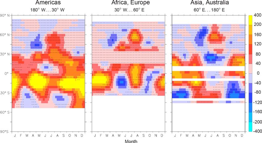
Figure 1. Inter-annual climate sensitivity γNEE-T in (gC m−2 yr−1 ) K−1 shown as Hovmöller diagrams: longitudinal averages of γNEE-T are
plotted as colour over latitude (vertical) and month of the year (horizontal). The stippling indicates robustness: crosses mark values with
absolute deviations ≤ 40 (gC m−2 yr−1 ) K−1 (one colour level) of all sensitivity cases from the base case.
This yields sensitivities as regression slopes gNEE-T EC = 3 Results
EC EC
1NEE / 1T . We also calculated the confidence inter-
val of the slope for the confidence level 90%, reflecting the 3.1 How does the inter-annual climate sensitivity
EC
uncertainty of gNEE-T given the scatter of the monthly values γNEE-T vary in space and by season?
around a linear relationship.
The sensitivities γNEE-T from the inversion and As a starting point, we present the results of the NEE–T in-
EC
gNEE-T from the explicit linear regression are not fully version in terms of γNEE-T , which is the local regression co-
comparable mathematically because (i) the time period (and efficient between inter-annual variations in NEE and temper-
to some extent the frequency filtering) are different, and ature, resolved seasonally (Sect. 2.2). As γNEE-T not only re-
(ii) the explicit linear regression of the total NEE is not only flects direct temperature responses but also responses to other
influenced by the year-to-year variations but also by the environmental variables that co-vary with temperature (such
ratio of NEE trend and temperature trend, while γNEE-T has as water availability, incoming solar radiation), we refer to it
deliberately been made insensitive to the trend (Sect. 2.2). as inter-annual climate sensitivity.
Therefore, we also calculated sensitivities gNEE-T Inv from Figure 1 presents the seasonal and spatial patterns of
the total monthly mean non-fossil CO2 flux (i.e. including the inter-annual climate sensitivity as Hovmöller diagrams
regression and residual terms of Eq. 2) and the employed showing longitudinally averaged γNEE-T with dependence
temperature field of the inversions in the same way and on latitude and month of the year. The longitudinal aver-
subsampled at the same months as for the EC data. A perfect age is taken separately over North and South America (left
match between gNEE-TEC Inv
and gNEE-T cannot be expected nev- panel), Europe and Africa (middle panel), and Asia and Aus-
ertheless because (iii) sensitivities from the inversion even tralia (right panel). This representation summarizes the es-
at its smallest resolved scale – the pixel scale – represent a sential variations of γNEE-T , as it is found to be relatively uni-
mixture of ecosystem types in unknown proportions, while form across longitude within the individual continents (not
the EC data represent a specific ecosystem type, (iv) NEE shown).
from the inversion includes the effects of disturbances such In essentially all northern extratropical land areas (north
as fire, which are absent from the EC data, and (v) there may of about 35◦ N), we estimate negative γNEE-T in spring (and
be local trends in the ecosystem behaviour observed by the to a lesser extent autumn), which is consistent with photo-
EC data due to ageing or slow species shifts, which average synthesis being temperature limited such that higher-than-
out on the larger spatial scales seen by the atmospheric normal temperatures lead to more negative NEE (i.e. larger-
inversion. than-normal CO2 uptake) and vice versa. Warmer conditions
tend to coincide with higher incoming solar radiation in May
Biogeosciences, 15, 2481–2498, 2018 www.biogeosciences.net/15/2481/2018/C. Rödenbeck et al.: How does the terrestrial carbon exchange respond to climatic variations? 2487
(a) Land total (d) Land total
4 CO2 flux
3
0.5
2
1
0.9
0
-1
-2
1990 2000 2010 0.0 0.5 1.0
(b) Land 25° N–90° N (e) Land 25° N–90° N
2
CO2 flux (PgC yr -1 )
CO2 flux
1
0.5
0
-1 0.9
-2
-3
(c) Land 90° S–25° N (f) Land 90° S–25° N
4 CO2 flux
3
0.5
2
1 Standard inversion
0.9
0 NEE-T inversion
NEE-T inv., sensit. cases
-1
-2
1990 2000 2010 0.0 0.5 1.0
Year (A.D.) Rel. SD
Figure 2. (a, b, c) Inter-annual anomalies of NEE integrated over all land (a), northern extratropical land (b), and tropical plus southern
land (c) as estimated by the standard inversion (Sect. 2.1, black) and different runs of the NEE–T inversion (Sect. 2.2, orange). The grey
band comprises the results of the sensitivity cases. (d, e, f) Taylor diagrams quantifying the agreement between the NEE–T inversions and
the standard inversion. Due to the construction of the Taylor diagram (Taylor, 2001), the horizontal position of a point gives the relative
fraction of the reference signal present in the test time series, while the vertical distance of this point from the horizontal axis gives the
relative amplitude (temporal standard deviation) of any additional signal components uncorrelated with the reference signal.
and/or June in the northern extratropics (according to a cor- extratropics may conceivably arise because the much smaller
relation analysis of CRUNCEPv7 data, not shown), which land area involves a much smaller number of degrees of free-
would tend to amplify the direct temperature effect. In sum- dom available to satisfy the data constraints (remember that
mer when photosynthesis is no longer limited by tempera- the oceanic flux cannot be adjusted in this inversion, while
ture, we find positive γNEE-T values. Such positive γNEE-T is the pCO2 -based ocean prior flux is actually less well con-
consistent with enhanced respiration in warmer summers, but strained in the southern extratropics due to the much smaller
also with the fact that warmer-than-normal periods are often density of pCO2 data).
also drier, leading to reduced photosynthetic uptake or en-
hanced fire activity. In winter, NEE is not found to respond 3.2 How much inter-annual variability of NEE can be
much to inter-annual climate variations. The interpretation reproduced by the seasonally resolved linear
of the seasonality of γNEE-T is confirmed by its latitude de- regression to T ?
pendence: consistent with the later spring and shorter sum-
mer in the higher northern latitudes, the period of negative The assumed linear relationship between NEE anomalies and
γNEE-T starts later there, and the period of positive γNEE-T is air temperature anomalies around their respective seasonal
shorter. cycles represents a strong abstraction of the complex under-
In the tropics, we find stronger and less systematic varia- lying physiological and ecosystem processes. Nevertheless,
tions in γNEE-T . However, as indicated by the missing stip- the inter-annual variations of global total NEE estimated by
pling, we also find larger disagreement between our sensitiv- the NEE–T inversion are very similar to those estimated by
ity cases designed to embrace plausible ranges for the essen- the standard inversion (Fig. 2a). The agreement is confirmed
tial inputs and parameters in the algorithm (Sect. 2.3). This by high correlation (Fig. 2d). For interpretation, we note that
reveals that the seasonal variations in γNEE-T are of limited variations in the global total CO2 flux are very well con-
robustness here. Nevertheless, a clear feature in the tropics is strained from atmospheric CO2 observations at timescales
the dominance of positive γNEE-T values. longer than the atmospheric mixing time (about 4 years)
In southern extratropical America and Africa, the seasonal (Ballantyne et al., 2012). Variations on the year-to-year scale
pattern has similarities with the northern extratropical pattern are already tightly constrained (Peylin et al., 2013). We thus
shifted by 6 months. The pattern in Australia is difficult to in- use the global CO2 flux from the standard inversion with ex-
terpret, but also not very robust. Larger errors in the southern plicit inter-annual degrees of freedom as a benchmark. Since
the ocean flux is identical in both the standard and NEE–T
www.biogeosciences.net/15/2481/2018/ Biogeosciences, 15, 2481–2498, 20182488 C. Rödenbeck et al.: How does the terrestrial carbon exchange respond to climatic variations?
CA-Man (ENF) FI-Hyy (ENF) FI-Sod (ENF) RU-Fyo (ENF) DK-ZaH (GRA) RU-Cok (OSH)
300 300 300 300 300 300
150 150 150 150 150 150
0 0 0 0 0 0
-150 -150 -150 -150 -150 -150
-300 -300 -300 -300 -300 -300
CH-Dav (ENF) DE-Tha (ENF) FR-LBr (ENF) IT-Lav (ENF) IT-Ren (ENF) IT-SRo (ENF) NL-Loo (ENF)
300 300 300 300 300 300 300
150 150 150 150 150 150 150
0 0 0 0 0 0 0
-150 -150 -150 -150 -150 -150 -150
-300 -300 -300 -300 -300 -300 -300
BE-Bra (MF) BE-Vie (MF) US-PFa (MF) US-Syv (MF) US-Me2 (ENF) US-NR1 (ENF)
300 300 300 300 300 300
150 150 150 150 150 150
0 0 0 0 0 0
Inter-annual climate sensitivity (gC/m2/yr/K)
-15 0 -150 -150 -150 -150 -150
-300 -300 -300 -300 -300 -300
DE-Hai (DBF) DK-Sor (DBF) IT-Col (DBF) US-Ha1 (DBF) US-MMS (DBF) US-WCr (DBF) US-UMB (DBF)
300 300 300 300 300 300 300
150 150 150 150 150 150 150
0 0 0 0 0 0 0
-150 -150 -150 -150 -150 -150 -150
-300 -300 -300 -300 -300 -300 -300
FR-Pue (EBF) IT-Cpz (EBF) US-Los (WET) US-Ton (WSA) US-Var (GRA)
300 300 300 300 300
150 150 150 150 150
0 0 0 0 0
-150 -150 -150 -150 -150
-300 -300 -300 -300 -300
GF-Guy (EBF) ZA-Kru (SAV) AU-How (WSA) AU-Tum (EBF)
300 300 300 300
150 150 150 150
0 EC data, lin. regression 0 0 0
NEE-T inversion
-150 NEE-T inv., sensit. cases -150 -150 -150
-300 -300 -300 -300
Jan Jul Jan Jan Jul Jan Jan Jul Jan Jan Jul Jan Jan Jul Jan
Figure 3. Comparison between the inter-annual climate sensitivities calculated from the inversion and from eddy covariance (EC) data for
EC
various sites with longer EC records. Black dots give the sensitivities gNEE-T calculated by the linear regression of monthly EC CO2 flux
data (FLUXNET2015 data set) against monthly air temperature co-measured at the flux towers (months with data in only 6 years or less are
discarded). The error bars around the dots comprise the confidence intervals of the regression slopes (at the 90 % confidence level); if the
confidence interval is above 300 (gC m−2 yr−1 ) K−1 (i.e. larger than the typical seasonal range), the corresponding dot is hollow. Orange and
grey lines give the sensitivities γNEE-T taken directly from various NEE–T inversions (base and sensitivity cases as in Fig. 2) at the respective
pixels enclosing the EC site locations. To allow for a more direct comparison between NEE–T inversion results and EC data, sensitivities for
the inversion (base case) have also been calculated by linear regression from the total monthly mean non-fossil CO2 flux and the temperature
field employed in the inversions in the same way and subsampled at the same months as for the EC data; these gNEE-T Inv values are shown as
orange dots. Panels are roughly ordered by latitude and land cover type (DBF: deciduous broadleaf forest, EBF: evergreen broadleaf forest,
ENF: evergreen needleleaf forest, GRA: grassland, MF: mixed forest, OSH: open shrubland, SAV: savanna, WET: permanent wetland, WSA:
woody savanna). See Table 2 for EC site locations.
inversion runs, the high level of agreement in Fig. 2 (panels a tudes, these two NEE contributions are expected to be rela-
and d) means that the spatially and seasonally resolved linear tively well constrained by atmospheric data independently of
NEE–T regression already provides a good approximation of each other. The linear approximation of the NEE–T inversion
global inter-annual NEE variations. is able to distinguish extratropical and tropical behaviour.
Almost the same level of agreement is also found for a For a further split into smaller regions, in particular along
split of the global NEE into a northern extratropical and a longitude, inter-annual NEE variations from standard and
tropical plus southern extratropical contribution (Fig. 2b, c NEE–T inversions stay similar, but deviations get larger (not
and e, f). Due to the faster atmospheric mixing within the ex- shown). This could indicate that the limits of the linear NEE–
tratropical hemispheres compared to the mixing across lati- T relationship start to kick in at these scales. However, the
Biogeosciences, 15, 2481–2498, 2018 www.biogeosciences.net/15/2481/2018/C. Rödenbeck et al.: How does the terrestrial carbon exchange respond to climatic variations? 2489
NEE variations can no longer be expected to be well con- scale NEE variability because DBF ecosystems only
strained from the atmospheric data at the regional scale. cover 11 to 25 % of the area around the sites shown.
Thus, the discrepancy can also be caused by the standard in-
version, while the NEE–T inversion could be the more real- – Generally good consistency within the confidence in-
istic one by profiting from the pixel-scale information added terval is also found at sites of various other ecosystem
through the temperature field, as discussed in Sect. 4.1. types in temperate northern latitudes (line 5).
– At the tropical and southern extratropical sites (last
3.3 Are the estimated patterns of γNEE-T compatible line), the comparison does not yield conclusive infor-
with ecosystem-scale eddy covariance data? mation, because the confidence intervals of the regres-
sion are much larger than the seasonal variations of both
Figure 3 compares inter-annual climate sensitivities (ordi-
inversion and EC results. We can only state that the
nate) calculated by the NEE–T inversion with those calcu- Inv EC
gNEE-T and gNEE-T sensitivities do not contradict each
lated independently from eddy covariance (EC) data for each
other statistically. Some qualitative consistency is found
month of the year (abscissa). Each panel represents an EC
at the Australian EBF site, even though the dominant
site roughly arranged by ecosystem types and latitudes. The
vegetation round the site is shrubland (about 45 %).
orange line with the surrounding grey band gives the sensi-
tivities γNEE-T from the various NEE–T inversion runs as in Though this comparison partly remains inconclusive (as the
Fig. 2 taken at the respective pixels enclosing the EC sites. confidence intervals at tropical and Southern Hemispheric
EC
The black dots are the sensitivities gNEE-T calculated by the Inv EC
sites are large, as gNEE-T and gNEE-T are not actually fully
explicit linear regression of monthly EC flux records against comparable (Sect. 2.4), and as by far not all areas and dom-
the co-measured monthly air temperature (Sect. 2.4). inating ecosystem types are represented), it does support the
To allow for a fairer comparison between inversion re- results of the NEE–T inversion, at least in the northern ex-
sults and EC data, additional colour dots give sensitivities tratropics.
Inv
gNEE-T calculated from the NEE–T inversion results in the
same way and subsampled at the same months as for the
EC data (Sect. 2.4). At most EC sites, the sensitivities cal- 4 Discussion
culated by the inversion itself (γNEE-T , orange lines) or by
Inv 4.1 NEE variations in the northern extratropics
explicit regression afterwards (gNEE-T , orange dots) mostly
agree within the confidence interval of the regression. This Given that we found robust seasonal patterns of
shows that the comparison of inversion and EC sensitivities γNEE-T which can be interpreted in terms of the fundamental
is meaningful despite their differences in meaning and calcu- physiological processes (Sect. 3.1), that these patterns are
lation (in particular, the trend influence (issue ii in Sect. 2.4) compatible with inferences from independent ecosystem-
Inv
on gNEE-T turns out to be relatively small because the ex- scale eddy covariance (EC) measurements (Sect. 3.3), and
plicit regressions are only done over the limited time period that the corresponding inter-annual NEE variations are
spanned by the EC records). compatible with the atmospheric constraint on the most
Despite their completely independent sources of informa- reliable large scales (Sect. 3.2), we conclude that the linear
tion and their remaining incompatibilities (Sect. 2.4), the sen- dependence of NEE anomalies on air temperature anomalies
sitivities from the EC data and the atmospheric NEE–T in- (as climate proxy) represents a meaningful approximative
version have a similar order of magnitude and similar sea- empirical description of the northern extratropical biosphere.
sonal patterns for a majority of EC sites (Fig. 3). For most The compatibility of the NEE–T relationships inferred from
sites and months, the sensitivities agree within their confi- large-scale atmospheric constraints and the ecosystem-scale
dence intervals. The level of agreement roughly depends on EC constraints of dominating vegetation types suggests
ecosystem type and latitude. that the regional or continental NEE variations are to a
– Generally good consistency is found in high northern substantial degree due to local variations linked to local
latitudes (line 1 of panels in Fig. 3) and at evergreen climate anomalies; otherwise the NEE–T inversion could not
needleleaf forest (ENF) sites in temperate northern lati- have worked. Given that, we expect the NEE–T inversion
tudes (line 2 and rightmost part of line 3). to provide more realistic inter-annual NEE variations on
regional scales than the standard inversion, which smoothly
– At mixed forest (MF) and deciduous broadleaf forest interpolates NEE on scales smaller than station-to-station
(DBF) sites in temperate northern latitudes (left part of differences (compare to the last paragraph of Sect. 3.2).
line 3 and line 4), consistency is mostly good as well, Note that as EC data measure fluxes on small spatial scales
though some months in spring or summer have more (a few hundreds of metres), the EC flux variations them-
Inv
negative gNEE-T sensitivities from EC data (e.g. DE- selves cannot directly be compared to the inversion results
Hai, DK-Sor, BE-Bra). However, the behaviour of DBF representing NEE over (sub)continental scales and integrat-
ecosystems is not an important contribution to larger- ing over many ecosystem types and climate regimes. In con-
www.biogeosciences.net/15/2481/2018/ Biogeosciences, 15, 2481–2498, 20182490 C. Rödenbeck et al.: How does the terrestrial carbon exchange respond to climatic variations?
trast to the fluxes, however, derived relationships (such as 4.3 An extended benchmark for process models
the NEE–T relationships considered here) may well be able
to bridge this scale gap. Data-based empirical relationships between inter-annual
Besides the inter-annual variations, the NEE–T inversion NEE variations and air temperature variations have been pro-
also reproduces the small negative trend in NEE through posed in the literature as benchmarks to evaluate biogeo-
adj chemical process models. For example, Cox et al. (2013)
its residual term fNEE,Trend in Eq. (2) (Fig. 2). Likewise,
it reproduces the northern extratropical increase in seasonal calculated an effective global climate sensitivity of 5.1 ±
adj
cycle amplitude through its residual term fNEE,SCTrend (not 0.9 PgC yr−1 K−1 over 1960–2010 by regressing the annual
shown). CO2 growth rate observed at the station Mauna Loa (Hawaii)
(taken as a proxy for the global total CO2 flux) against
4.2 NEE variations in the tropics 30◦ N–30◦ S (both land and ocean) averaged air tempera-
ture (after detrending both time series by subtracting an
In contrast to the northern extratropics, we did not find 11-year running mean). In a similar way (using the aver-
conclusive seasonal patterns of γNEE-T in the tropics age atmospheric growth rate from a varying set of back-
(Sect. 3.1). However, despite the substantial uncertainty ground sites, a slightly different time series treatment, and
range of γNEE-T (Fig. 1), the sensitivity cases reproduce al- 24◦ N–24◦ S land temperature), Wang et al. (2013) obtained a
most identical inter-annual NEE variations in the tropics (see value of 3.5±0.6 PgC yr−1 K−1 over 1959–2011. Wang et al.
the narrow grey band around the NEE–T estimate in Fig. 2c). (2014) regressed the mean Mauna Loa and South Pole CO2
This underlines the fact that pan-tropical NEE variations are growth rates against 23◦ N–23◦ S vegetated land temperature
actually well constrained from the atmospheric data, while over moving 20-year windows and reported effective global
the seasonal differences in γNEE-T arise to compensate for the climate sensitivities between 3.4 ± 0.4 PgC yr−1 K−1 (dur-
set-up differences among the sensitivity cases. As shown be- ing 1960–1979) and 5.4 ± 0.4 PgC yr−1 K−1 (during 1992–
low (Sect. 4.3), all the seasonally different γNEE-T estimates 2011).
correspond to a similar effective sensitivity (having a positive The inversion results presented here allow us to extend
value) on yearly timescales. Due to this, the NEE–T inver- these benchmarks in two ways. As a first extension, we can
sion is found to possess predictive skill on the timescale of evaluate to what extent the inter-annual variations in local or
the El Niño–Southern Oscillation (Rödenbeck et al., 2018). averaged atmospheric CO2 growth rates are indeed equiva-
The positive effective γNEE-T in the tropics (Sect. 3.1) lent to the inter-annual variations in the global total CO2 flux
is consistent with the strong positive correlation of atmo- (as implicitly assumed in the above-mentioned studies) and
spheric CO2 growth with large-scale tropical annual tem- to what extent the global total CO2 flux is indeed representa-
perature (Wang et al., 2013). This is unlikely to arise from tive of global terrestrial NEE or, even more specifically, trop-
a direct temperature effect, however, because process stud- ical NEE. This can be evaluated here because all these time
ies (e.g. Meir et al., 2008; Bonal et al., 2008; Alden et al., series (spatially explicit CO2 fluxes with all their contribu-
2016) point to water availability rather than temperature as tions, as well as the corresponding atmospheric CO2 varia-
the dominant control on the ecosystem scale. This is also tions at the measurement stations) are available within the
confirmed by the large confidence intervals of the NEE–T inversion calculation. To ensure a mutually consistent treat-
regression of the EC data from the only tropical site available ment of these time series, we used running yearly averages
here (GF-Guy, leftmost on last line of Fig. 3). A strong corre- (January through December, February through next January,
lation with temperature can still arise statistically due to the etc.) of the flux time series and running yearly differences
strong link of temperature and precipitation anomalies over (next January minus January, next February minus February,
larger spatial scales (Berg et al., 2014). Moreover, the vapour etc., multiplied by 2.12 PgC ppm−1 ; Ballantyne et al., 2012)
pressure deficit (VPD) controlling photosynthesis responds of the atmospheric CO2 time series. All these inter-annual
particularly strongly to temperature variations in the warm time series were then regressed over 1985–2016 against an-
tropical climate due to the non-linearity of the VPD(T) de- nual tropical land temperature (25◦ N–25◦ S) derived from
pendence (Monteith and Unsworth, 1990). Further, T is spa- the same temperature field without decadal variations as used
tially coherent over much larger areas in the tropics, while in the NEE–T inversion. The resulting effective climate sen-
variability in water availability is local and averages out over sitivities are shown in Fig. 4. The sensitivities of the total
larger spatial scales (Jung et al., 2017). Nevertheless, a direct CO2 flux (solid bars in the middle) calculated from the stan-
temperature effect in the tropics was found by Clark et al. dard inversion (black) or from the NEE–T inversion (orange)
(2013), at least for a component flux of NEE (wood produc- are similar to each other and fall in between the values by
tion) in 12-year plot data. Cox et al. (2013) and Wang et al. (2013). Part of the discrep-
ancies between these results can be attributed to the different
time periods and the different time series treatments (in par-
ticular, to the extent to which decadal variability has been
removed). Figure 4, however, reveals another reason for the
Biogeosciences, 15, 2481–2498, 2018 www.biogeosciences.net/15/2481/2018/C. Rödenbeck et al.: How does the terrestrial carbon exchange respond to climatic variations? 2491
discrepancies: the sensitivity of the Mauna Loa growth rate
(middle hashed blue bar) is larger than that of the global flux
Glob. NEE (NEE-T inv.)
BRW gr. r. (NEE-T inv.)
Trop. NEE (NEE-T inv.)
MLO gr. r. (NEE-T inv.)
SPO gr. r. (NEE-T inv.)
Glob. flux (NEE-T inv.)
Glob. NEE (std. inv.)
BRW gr. r. (std. inv.)
Trop. NEE (std. inv.)
MLO gr. r. (std. inv.)
SPO gr. r. (std. inv.)
Glob. flux (std. inv.)
(solid bars). This cannot be due to a deficiency in the in-
BRW gr. r. (obs.)
MLO gr. r. (obs.)
SPO gr. r. (obs.)
versions to fit Mauna Loa’s variability because the modelled
Mauna Loa sensitivities (hashed bars next to the middle blue
bar) agree well with the observed ones. Thus, a sensitivity
calculated from the Mauna Loa growth rate (as in Cox et al.,
2013) somewhat overestimates the sensitivity of the global
flux. The Mauna Loa sensitivity is still much closer to that of 7
the global CO2 flux than sensitivities calculated from most 6
Regr. slope
other stations: southern extratropical stations like the South 5
Pole (or the mean of Mauna Loa and the South Pole as in 4
Wang et al., 2014) lead to a substantial underestimation (it is 3
2
unclear why the sensitivity reported by Wang et al. (2014) for
1
the recent 1992–2011 period is nevertheless even higher than 0
our Mauna Loa value), while northern extratropical stations
like Point Barrow lead to an even stronger overestimation Figure 4. Effective large-scale inter-annual climate sensitivities
than Mauna Loa. This suggests that using a varying mixture (PgC yr−1 K−1 ) calculated from the standard inversion (black),
of stations (as in Wang et al., 2013) can induce further er- from the NEE–T inversion (orange), or from observed atmospheric
rors, in particular when possible changes in sensitivity are CO2 (blue). The sensitivities refer to inter-annual variations in the
considered. We note that the atmospheric inversions bene- CO2 growth rate at three selected atmospheric stations (Point Bar-
fit from using multiple station records because the transport row, Alaska (BRW), Mauna Loa, Hawaii (MLO), and the South
model links the atmospheric CO2 signals to their different Pole (SPO), diagonally hashed), in the global total CO2 exchange
(solid bars), in the global terrestrial NEE (horizontally hashed), or in
areas of origin rather than the instantaneous link of the atmo-
tropical NEE (25◦ N–90◦ S, vertically hashed), all regressed against
spheric signals to the global flux as in the direct use of station inter-annual variations in air temperature averaged across tropical
records. land (25◦ N–25◦ S) over 1985–2016. The red line surrounded by
Care is also needed in the interpretation of the estimated grey shading denotes the result 5.1±0.9 PgC yr−1 K−1 by Cox et al.
effective sensitivities: the sensitivity of the total CO2 flux (2013), even though it is calculated in a slightly different way.
(solid bars) underestimates that of global NEE only (hori-
zontally hashed bars) because the ocean flux is substantially
anti-correlated with NEE on the inter-annual timescale. The (Sect. 3.1), this offers a much more detailed benchmark of the
sensitivity of tropical-only NEE (vertically hashed bars) is process representation in the models than the existing single-
smaller than that of global NEE, though the reduction is less valued effective climate sensitivity of the global CO2 growth
than according to the ratio of land area, confirming the dom- rate. For the tropics, unfortunately γNEE-T is not constrained
inance of tropical NEE variations. well enough to do that, but due to the fact that pan-tropical
As a second extension of process model benchmarking, NEE variations are nevertheless quite robust (Sect. 4.2), the
the data-based estimates of the spatially and seasonally re- effective climate sensitivity of tropical NEE from Fig. 4
solved γNEE-T from the NEE–T inversion can directly be em- (4.2 PgC yr−1 K−1 with a range across the sensitivity cases of
ployed as target values by regressing the NEE simulated by 3.8. . .4.4 PgC yr−1 K−1 ) may be used as a specifically tropi-
the terrestrial biosphere or Earth system model against the cal target instead.
model temperature for individual small regions and seasons
across the years 1985–2016 and comparing these model- 4.4 Could the results be improved by using a
derived local and season-specific sensitivities to the data- multivariate regression against further climatic
based values presented here (using the ensemble of sensi- variables?
tivity cases as a measure of uncertainty in γNEE-T ). Impor-
tantly, before regressing, the model NEE and temperature We also tested the algorithm with precipitation (P ) or so-
fields need to be deseasonalized, detrended, and filtered in lar radiation as explanatory variables, individually or in mul-
the same way as done for the observed temperature in the tivariate combinations (not shown). While, for example, an
NEE–T inversion (Sect. 2.2) because the numerical γNEE-T NEE–P inversion had almost as good an explanatory power
values are somewhat specific to the chosen filtering, in par- as the NEE–T inversion, a multivariate NEE–T –P inversion
ticular to the exact way to remove decadal variations (as did not explain much more NEE variations than the univari-
is also the case for the effective global climate sensitivity ate NEE–T inversion did already. This confirms the strong
targets by Cox et al., 2013, and Wang et al., 2013, 2014). background correlations of air temperature with the other cli-
For the northern extratropics, where γNEE-T is quite robustly mate variables on inter-annual timescales. It also means that
constrained and shows distinct spatial and seasonal patterns a multivariate regression would – despite a mathematically
www.biogeosciences.net/15/2481/2018/ Biogeosciences, 15, 2481–2498, 20182492 C. Rödenbeck et al.: How does the terrestrial carbon exchange respond to climatic variations?
unique partitioning into contributions of the individual ex- The results of the NEE–T inversion can be applied to
planatory variables – likely not yield a uniquely interpretable benchmark process models of the land biosphere or Earth
attribution of NEE variability to different causes. system models: the spatially and seasonally resolved inter-
Given that, a univariate NEE–T inversion seems advan- annual climate sensitivity γNEE-T can be calculated from the
tageous because T likely has data sets best constrained by model output (using detrended NEE over the period 1985–
observations. As a regression is confined to the variability 2016 for consistency) and compared to the values presented
present in the explanatory variables, using less well-observed here; this allows for a more detailed benchmark for the north-
or even modelled variables (as would be the case for precip- ern extratropical ecosystem processes than existing effective
itation or cloud cover) involves the risk of contamination. global sensitivities. Further, as its adjustable degrees of free-
dom are identically applied every year, the regression of-
fers a way to bridge temporal gaps in the atmospheric CO2
5 Conclusions and outlook records; it transfers information from the recent data-rich
years into the more data-sparse past. Similarly, the NEE–T
The response of net ecosystem exchange (NEE) to climate
regression allows us to forecast the CO2 flux for some years
anomalies has been estimated by linear regression against
if forecasted air temperatures (and extrapolations of fossil
anomalies in air temperature (T ) within an atmospheric in-
fuel emissions and the ocean exchange) are available. As an-
version based on a set of long-term atmospheric CO2 ob-
other application, the regression may help to uncover smaller
servations. The resulting spatially and seasonally resolved
decadal trends in the atmospheric CO2 signal by separating
regression coefficients γNEE-T are interpreted as an inter-
them from the larger inter-annual responses of NEE. By ex-
annual climate sensitivity comprising the direct tempera-
tending the calculation to the full period of atmospheric CO2
ture response as well as responses to co-varying anomalies
measurements (since the late 1950s; see Rödenbeck et al.,
in other environmental conditions (e.g. moisture, radiation)
2018), we can investigate possible decadal changes in the
(Sect. 4.4).
inter-annual climate sensitivity γNEE-T .
– The inferred inter-annual climate sensitivity
γNEE-T shows distinct and interpretable patterns
Data availability. The inversion results are available for use in col-
along latitude and season. In particular, we find neg-
laborative projects from the Jena CarboScope website at http://
ative γNEE-T during spring and autumn (consistent
www.BGC-Jena.mpg.de/CarboScope/ (http://dx.doi.org/10.17871/
with a temperature-limited photosynthesis) and positive CarboScope-s85oc_v4.1s, Rödenbeck and Heimann, 2017a; http://
γNEE-T during summer (consistent with a water-limited dx.doi.org/10.17871/CarboScope-s04XocNEET_v4.1s, Rödenbeck
photosynthesis) in all northern extratropical ecosystems and Heimann, 2017b).
(Sect. 3.1).
– Despite the complexity of the underlying plant and
ecosystem processes, the spatially and seasonally re-
solved linear regression of NEE against temperature
anomalies (taken as climate proxy) fitted to atmospheric
CO2 data can reproduce a large fraction of inter-annual
variations in the NEE, at least in the northern extrat-
ropics. This conclusion is based on the agreement of
the inferred NEE variations with a time-explicit atmo-
spheric inversion at well-constrained large spatial scales
(Sect. 3.2) and the consistency of γNEE-T with indepen-
dent calculations from eddy covariance data at small
spatial scales (Sect. 3.3). Among the reasons for this po-
tentially surprising finding is that the regression is only
applied to the inter-annual anomalies of NEE around its
mean seasonal cycle (rather than to the full range of sea-
sonal temperature variations) and that the different be-
haviours in different seasons have been accounted for.
Biogeosciences, 15, 2481–2498, 2018 www.biogeosciences.net/15/2481/2018/You can also read