How Individuals Smooth Spending: Evidence from the 2013 Government Shutdown Using Account Data
←
→
Page content transcription
If your browser does not render page correctly, please read the page content below
How Individuals Smooth Spending:
      Evidence from the 2013 Government Shutdown
                             Using Account Data∗
      Michael Gelman†              Shachar Kariv‡             Matthew D. Shapiro§
                                            ¶
                       Dan Silverman                  Steven Tadelisk

                                   February 2015
                              Revised October 14, 2015

                                           Abstract

          Using comprehensive account records, this paper examines how individuals
      adjusted spending and saving in response to a temporary drop in income due to
      the 2013 U.S. government shutdown. The shutdown cut paychecks by 40% for
      affected employees, which was recovered within 2 weeks. Though the shock was
      short-lived and completely reversed, spending dropped sharply implying a naı̈ve
      estimate of the marginal propensity to spend of 0.58. This estimate overstates
      how consumption responded. While many individuals had low liquidity, they
      used multiple strategies to smooth consumption including delay of recurring
      payments such as mortgages and credit card balances.

  ∗
     We thank Kyle Herkenhoff, Patrick Kline, Dimitriy Masterov, Melvin Stephens Jr., and Jeffrey
Smith as well as participants at many seminars for helpful comments. This research is supported
by a grant from the Alfred P. Sloan Foundation. Shapiro acknowledges additional support from the
Michigan node of the NSF-Census Research Network (NSF SES 1131500).
   †
     University of Michigan, mgelman@umich.edu
   ‡
     UC Berkeley, kariv@berkeley.edu
   §
     University of Michigan and NBER, shapiro@umich.edu
   ¶
     Arizona State University and NBER, Daniel.Silverman.1@asu.edu
   k
     UC Berkeley, NBER, and CEPR, stadelis@berkeley.edu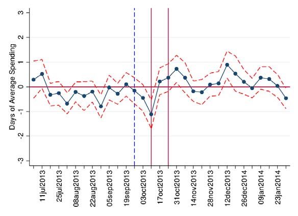
“Unless we get our paychecks this coming Monday we don’t have the
      money to cover our mortgage, car payment, and the rest of the bills that
      we need to pay.” — ABC 7 news

1     Introduction
How consumers respond to changes in income is a central concern of economic anal-
ysis and is key for policy evaluation. This paper uses the October 2013 U.S. Federal
Government shutdown and a newly developed dataset of financial account records
to examine how consumers with different levels of liquidity, income, and spending
respond to a short-lived and entirely reversed drop in income. For affected govern-
ment employees, the shutdown caused a sharp decline in income that was recovered
within two weeks. The new dataset, derived from the de-identified account records
of more than 1 million individuals living in the United States, provides a granular
and integrated view of how individuals in different economic circumstances adjusted
spending, saving, and debt in response to the shock.
    The most important findings are, first, that many workers routinely have very low
levels of liquidity, especially in the days just before their regular paycheck arrives. Sec-
ond, and consistent with low liquidity, spending by affected workers declined sharply
in response to the drop in income caused by the shutdown – though the drop lasted
at most two weeks and was then offset by an equal increase. Third, the granularity
and integration of the data reveal the means used by affected workers to smooth
consumption—if not spending—most notably their delay of recurring expenses such
as mortgage payments and credit card balances. Last, though many workers found
very low-cost ways to weather the shock, some with low liquidity who were already
relying on credit card debt accumulated still more credit card debt.
    Prior studies that measure the response of individuals to changes in income have
faced two challenges. First, the optimal reaction to an income change depends both on
whether the change is anticipated, and on its persistence; but standard data sources
make it difficult to identify shocks to expected income and the longevity of these
shocks. Second, analysis and policy prescriptions often require a comprehensive view
of the heterogeneous responses to an income change. Existing data typically capture

                                             1
only some dimensions with sufficient resolution. They may measure total spending
with precision, but not savings or debt; or they measure spending and debt well, but
do not measure income with similar accuracy.
       We overcome the challenge of identifying income shocks and their persistence
by using the 2013 U.S. Federal Government shutdown, which produced a significant,
temporary, and easily identified negative shock to the incomes of a large number of em-
ployees. We address the challenge of measuring a household’s full range of responses
to this shock by exploiting a new dataset derived from the integrated transactions
and balance data of more than 1 million individuals in the U.S.1
       More specifically, the data allow us to distinguish Federal government employees
subject to the shutdown. They are distinguished by the transaction description as-
sociated with direct deposit of their paychecks to their bank accounts. Knowing who
was subject to the income shock, we can examine their responses in terms of spend-
ing and other variables before, during, and after the government shutdown. These
responses are estimated by a difference-in-difference approach, where the outcomes of
affected government workers are compared with those of a control group consisting
of workers that have the same biweekly pay schedule as the Federal government, but
who were not subject to the shutdown. The control group is mainly non-Federal
workers, though also includes some Federal workers not subject to the shutdown.
       The pay of a typical affected worker was 40% below normal during the shutdown
because the government was closed from October 1 to October 16, 2013, thus including
the last four days of the previous ten-day pay period. By the next pay period,
however, government operations had resumed and workers were reimbursed fully for
the income lost during the shutdown. The transaction data clearly show this pattern
for affected workers. This event combined with the distinctive features of the data,
which link income, spending, and liquid assets at a high frequency for each individual,
provides an unusual opportunity to study the response to a relatively sizeable shock
that affected just the timing of income for individuals across the income distribution,
without any net effect on their lifetime incomes. See the related literature section
   1
    The data are captured in the course of business by a mobile banking app. While newly developed,
this dataset has already proved useful for studying the high-frequency response of spending to
regular, anticipated income by levels of spending, income, and liquidity (Gelman et al. 2014). The
related literature section below discusses other studies that use similar types of account data.

                                                2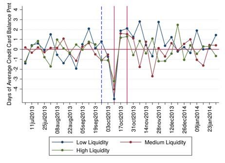
below for a discussion of the distinctions of this study.
   An important fact revealed by the balance records is that many affected employees
maintained low levels of liquid assets (checking and saving account balances), espe-
cially in the days just before their regular paychecks arrive. Prior to the shutdown,
the median worker in the data held an average liquid assets balance sufficient to cover
just eight days of average spending. Moreover, liquidity exhibits systematic changes
over the pay-cycle. Just before payday, the median level of liquidity is only five days
of average spending. Indeed, a substantial fraction of this population barely lives
paycheck-to-paycheck. On the day before their paycheck arrives, the bottom third of
the liquidity distribution has, on average, a liquid asset balance of zero.
   Given such low levels of liquidity, it is perhaps unsurprising that the transaction
records show a sharp drop in total spending by affected workers during the week of
missing paycheck income. Weekly spending declined by roughly half the reduction
in income and then recovered roughly equally over the two pay periods following the
end of the shutdown. Econometric analysis reveals a marginal propensity to spend
of about 0.58 as a response to the income shock. Most individuals reversed this drop
in spending immediately after they receive the paychecks that reimbursed them for
their lost income.
   On its face, it is troubling that so many affected workers maintained such low
liquidity and exhibited such a sharp spending response to an unexpected but brief
delay in income. It suggests either that benchmark theories founded on a taste for
smoothing consumption are badly specified; that households are inadequately buffered
against even very temporary shocks; or that the financial markets that make smooth-
ing possible are functioning poorly.
   Further examination of the data reveals, however, that even consumers with low
liquidity can smooth consumption better than spending using low-cost methods to
shift the timing of payments for committed forms of expenditure. More detailed
analysis shows that affected workers delayed mortgage payments, in particular; and
many individuals shifted credit card balance payments. At the same time, the data
show no increase in spending on credit cards; average debt only increased due to
delays in debt payments. Hence, while they responded to the temporary shock by
reducing spending, a large part of their reaction was to delay recurring payments

                                           3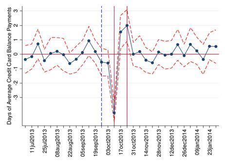
that impose little to no penalty. This shows how consumers make use of short-term
margins of adjustment that are mostly overlooked in the literature on methods of
smoothing consumption in response to at least temporary income shocks. As such,
it also reveals a potentially important welfare benefit of, especially, mortgages with
low interest rates. Mortgages can function as a (cheap) line of credit that can help
smooth even large, if brief, shocks to income at relatively low cost.
    While the data show that many affected workers were able to use perhaps uncon-
ventional means to smooth consumption, if not spending, for some with low liquidity
these methods were either inadequate or unavailable. This group, who was carrying
some credit card debt already, emerged from the shutdown with still more debt owing
to failure to make payments rather than new borrowing.
    The remainder of the paper proceeds as follows. Section 2 describes the paper’s
relationship to prior studies of individual responses to income shocks. Section 3
provides key facts about the circumstances surrounding the shutdown. Section 4
describes the data and our research design. It establishes that many workers regularly
have low liquidity prior to receiving their paycheck. Section 5 estimates the average
response of spending and liquid assets to the shock. Section 6 considers heterogeneity
in these responses across the liquidity distribution and examines the consequences for
credit card debt.

2     Related Literature
The literature concerned with individual responses to income shocks is large. Jap-
pelli and Pistaferri (2010) offer an insightful review. Relative to that large litera-
ture, a principal distinction of our paper is the integrated, administrative data that
allow accurate observation of liquidity, of the income shock itself, and of several
forms of response to the shock. These data thus provide measures of important
constraints and outcomes that allow improved inference from the heterogeneous and
multi-dimensional reactions to this change in income.
    Prior studies of income shocks have mostly relied on the self-reports of survey
respondents to provide information either about the shock or about the response of

                                           4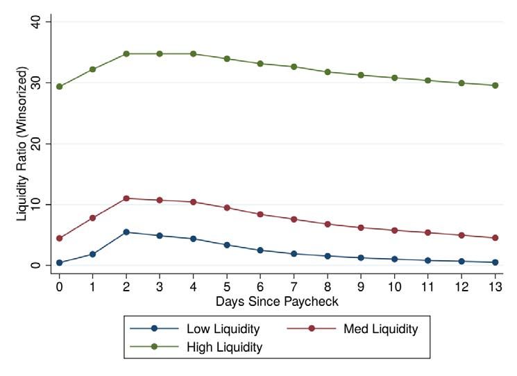
spending and savings and debt.2 Carroll, Crossley, and Sabelhaus (2013), Dillman
and House (2013), Einav and Levin (2014), and others, have called for increased use of
administrative records to augment survey research. So far, however, the administra-
tive records available for research have typically represented just a slice of economic
activity, either providing information about spending at just one retailer, or about
the use of a few credit cards, or about just one form of spending.3 Other approaches
blend survey and administrative data. For example, Broda and Parker (2014) and
Parker (2015) use consumer-based scanner data to study the response of spending to
an income shock; and use surveys for measuring income.4 This paper is different from
these studies of purely administrative data and from those of blended data sources:
The integrated data we use provide an accurate, high-resolution, and high frequency
picture of liquidity before the shock, and both the spending and net saving responses
to the shock.
       By using integrated account records, this paper is part of a new and still small
literature that includes Baker (2014), Kuchler (2014), Gelman et al. (2014), and Baker
and Yannelis (2015). Baker (2014) uses account records from an online banking app,
links them to external data on employers, and instruments for individuals’ income
changes with news about their employers. Because they are persistent, theory suggests
that some of these income shocks (from layoffs or plant closings, e.g.) should have
different implications for spending from the one caused by the government shutdown.
Nevertheless, like the present paper, Baker (2014) finds evidence of the importance of
liquidity (more than debt) for the spending response to an income shock. The present
paper is distinct in its study of the methods by which those with very little liquidity
smooth consumption through a temporary income shock.
       Kuchler (2014) studies integrated account records from an online financial man-
agement service that elicits from its customers plans for paying down credit card
debt. Kuchler (2014) uses those plans, along with the spending responses to income
changes, to evaluate a model of present-biased time preferences.
   2
     See, for example, Souleles (1999), Browning and Crossley (2001), Shapiro and Slemrod (2003),
and Johnson et al. (2006).
   3
     See, for example, Gross and Souleles (2002), Agarwal, Liu, and Souleles (2007), and Aguiar and
Hurst (2005).
   4
     Einav, Leibtag, and Nevo (2010) discuss the challenges that even scanner technologies like
Nielsen Consumer Panel (formerly Homescan), and Feenstra and Shapiro (2003) discuss the chal-
lenges of using store-based scanner data to measure expenditure and prices.

                                                5
Gelman et al. (2014) use a small subsample of the same data we use in this
paper to study the spending response to the arrival of predictable (paycheck and
Social Security benefit) income. That paper did not examine other outcomes besides
spending. Finally, in a complementary study completed shortly after ours, Baker
and Yannelis (2015) use data from the same banking app used in Baker (2014) to
describe the response of affected government workers to the 2013 shutdown. Baker
and Yannelis (2015) focuses on income and spending, but does not integrate those
outcomes with financial positions. Their analysis confirms that the spending and
income response to the government shutdown is identifiable in these data sets. From
these initial facts, their paper analyzes time allocation and home production. Our
paper focuses on the precarious liquidity position individuals find themselves in near
the end of the paycheck cycle and the different channels through which individuals
smoothed their consumption.
        The shutdown also is a distinctive shock. The shock is large, negative, and propor-
tional to income. These features stand in contrast to shocks arising from government
stimulus payments, which are positive and often weakly related to income. See, for
example, Shapiro and Slemrod (1995, 2003), Johnson et al. (2006), Parker et al.
(2013), Agarwal et al. (2007), Bertrand and Morse (2009), Broda and Parker (2014),
Parker (2015), and Agarwal and Qian (2014). The government shutdown caused a
40% drop in anticipated paycheck income for individuals across a wide range of the
income distribution. Thus, unlike the stimulus payments, the shutdown represented
a sizeable, albeit temporary, shock even to high-income households.

3         The 2013 U.S. Government Shutdown

3.1        Background
The U.S. government was shut down from October 1 to October 16, 2013 because
Congress did not pass legislation to appropriate funds for fiscal year 2014. While
Federal government shutdowns have historical precedent, it was difficult to anticipate
whether this shutdown would occur and how long it would last.5 The shutdown was
    5
    There have been 12 shutdowns since 1980 with an average length of 4 days. The longest previous
shutdown lasted for 21 days in 1995-1996. See Mataconis (2011).

                                                6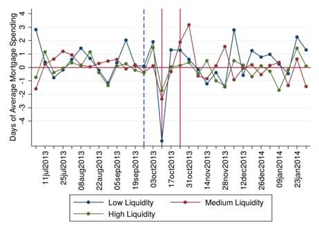
preceded by a series of legislative battles surrounding the Affordable Care Act (ACA),
also known as Obamacare. Key events and their timing are described in Figure 1.
       Opponents of the ACA in the House of Representatives sought to tie FY 2014
appropriations to defunding the ACA. They used the threat of a shutdown as a lever
in their negotiations and thus generated considerable uncertainty about whether a
shutdown would occur. Just days before the deadline to appropriate funding and
avoid a shutdown, there was substantial uncertainty over what would happen. A
YouGov/Huffington Post survey conducted on September 28-29, 2013 showed that
44% of U.S. adults thought Congress would reach a deal to avoid a shutdown while
26% thought they would not, and 30% were unsure. A similar survey taken after
the shutdown began on October 2-3, 2013 showed substantial uncertainty over its ex-
pected duration. 7% thought the shutdown would last less than a week, 31% thought
one or two weeks, 19% thought three or four weeks, and 10% thought the shutdown
would last more than a month. 33% were unsure of how long it would last.6 For
most federal employees, therefore, the shutdown and its duration were likely difficult
to anticipate at the outset. While it was not a complete surprise, it was a shock to
many that the shutdown did indeed occur. On the other hand, as we will discuss in
the next subsection, the shutdown was essentially resolved contemporaneously with
the receipt of the paycheck affected by the shutdown. Hence, there was no reason
based on permanent income to respond to the drop in income.

3.2       Impact on Federal Employees
Our analysis focuses on the consequences of the shutdown for a group of the approx-
imately 2.1 million federal government employees. The funding gap that caused the
shutdown meant that most federal employees could not be paid until funding legis-
lation was passed. The 1.3 million employees deemed necessary to protect life and
property were required to work. They were not, however, paid during the shutdown
for work that they did during the shutdown. The 800,000 “non-essential” employees
were simply furloughed without pay.7 In previous shutdowns, employees were paid
   6
    Each survey was based on 1,000 U.S. adults. See YouGov/Huffington Post (2013a, b).
   7
    Some federal employees were paid through funds not tied to the legislation in question and were
not affected. The Pentagon recalled its approximately 350,000 employees on October 5, reducing
the number of furloughed employees to 450,000.

                                                7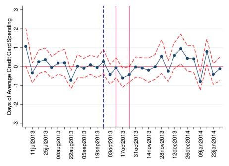
retroactively (whether or not they were furloughed). Of course, it was not entirely
clear what would happen in 2013. On October 5, however, the House passed a bill to
provide back pay to all federal employees after the resolution of the shutdown. While
not definitive, this legislation was strong reassurance that the precedent of retroactive
pay would be respected, as in fact it was when the shutdown concluded. After the
October 5 Congressional action, most of the remaining income risk to employees was
due to the uncertain duration of the shutdown and to potential cost-cutting measures
that could be part of a deal on the budget.
   Unlike most private sector workers, Federal workers are routinely paid with a lag
of about a week, so the October 5 House vote came before reduced paychecks were
issued. For most government employees, the relevant pay periods are September 22 -
October 5, 2013 and October 6 - October 19, 2013. Because the shutdown started in
the latter part of the first relevant pay period, employees did not receive payment for
5 days of the 14 day pay period. For most employees on a Monday to Friday work
schedule, this would lead to 4 unpaid days out of 10 working days, so they would
receive 40% less than typical pay. The actual fraction varies with hours and days
worked and because of taxes and other payments or debits. Since the government
shutdown ended before the next pay date, employees who only received a partial
paycheck were fully reimbursed in their next paycheck.
   Federal government employees are a distinctive subset of the workforce. Accord-
ing to a Congressional Budget Office report (CBO 2012), however, federal employees
represent a wide variety of skills and experiences in more than 700 occupations. Com-
pared to private sector employees, they tend to be older, more educated, and more
concentrated in professional occupations. Table 1 below reproduces Summary Ta-
ble 1 in the CBO report. Overall, total compensation is slightly higher for federal
employees. Breaking down the compensation difference by educational attainment
shows that federal employees are compensated relatively more at low levels of edu-
cation while the opposite holds for the higher end of the education distribution. In
the next section, we make similar comparisons based on Federal versus non-Federal
employees in our data. The analysis must be interpreted, however, with the caution
that Federal employees may not have identical behavioral responses as the general
population. We return to this issue in the discussion of the results.

                                           8
4         Data and Design

4.1        Data
The source of the data analyzed here is a financial aggregation and bill-paying com-
puter and smartphone application that had approximately 1.5 million active users in
the U.S. in 2013.8 Users can link almost any financial account to the app, including
bank accounts, credit card accounts, utility bills, and more. Each day, the application
logs into the web portals for these accounts and obtains key elements of the user’s
financial data including balances, transaction records and descriptions, the price of
credit and the fraction of available credit used.
        We draw on the entire de-identified population of active users and data derived
from their records from late 2012 until October 2014. The data are de-identified and
the analysis is performed on normalized and aggregated user-level data as described
in the Appendix. The firm does not collect demographic information directly and
instead uses a third party business that gathers both public and private sources of
demographics, anonymizes them, and matches them back to the de-identified dataset.
Appendix Table A (replicated from Table 1 of Gelman et al. 2014) compares the
gender, age, education, and geographic distributions in a subset of the sample to
the distributions in the U.S. Census American Community Survey (ACS) that is
representative of the U.S. population in 2012. The app’s user population is not
representative of the U.S. population, but it is heterogeneous, including large numbers
of users of different ages, education levels, and geographic locations.
        We identify paychecks using the transaction description of checking account de-
posits. Among these paychecks, we identify Federal employees by further details in
the transaction description. The appendix describes details for identifying paychecks
in general and Federal paychecks in particular. It also discusses the extent to which
we are capturing the expected number of Federal employees in the data. The number
of federal employees and their distribution across agencies paying them are in line
with what one would expect if these employees enroll in the app at roughly the same
    8
     We gratefully acknowledge the partnership with the financial services application that makes
this work possible. All data are de-identified prior to being made available to the project researchers.
Analysis is carried out on data aggregated and normalized at the individual level. Only aggregated
results are reported.

                                                   9
frequency as the general population.
4.2 Design: Treatment and Controls
Much of the following analysis uses a difference-in-differences approach to study how
Federal employees reacted to the effects of the government shutdown. The treatment
group consists of Federal employees whose paycheck income we observe changing
as a result of the shutdown. The control group consists of employees that have
the same biweekly pay schedule as the Federal government who were not subject
to the shutdown (see the Appendix for more details). The control group is mainly
non-Federal employees, but also includes some Federal employees not subject to the
shutdown.9 Table 2 shows summary statistics from the app’s data for these groups of
employees. As in the CBO study cited above, Federal employees in our sample have
higher incomes. They also have higher spending, higher liquid balances, and higher
credit card balances.
We use the control group of employees not subject to the shutdown to account
for a number of factors that might affect income and spending during the shutdown:
these include aggregate shocks and seasonality in income and spending. Additionally,
interactions of pay date, spending, and day of week are important (see Gelman et al.
2014). Requiring the treatment and control to have the same pay dates and pay date
schedule (biweekly on the Federal schedule) is a straightforward and important way
to control for these substantial, but subtle effects.
There is, of course, substantial variability in economic circumstance across indi-
viduals both within and across treatment and controls. We normalize many variables
by average daily spending, or where relevant by average account balances) at the
individual level. This normalization is a simple, and given the limited covariates in
the data, a practical way to pool individuals with very different levels of income and
9
Employees not subject to the shutdown include military, some civilian Defense Department, Post
Office, and other employees paid by funds not involved in the shutdown. An alternative strategy
would use just the Federal workers not affected by the shutdown as the control. We do not adopt
this strategy because we believe a priori that it is less suitable because the workers exempted from
the shutdown are in non-random agencies and occupations. This selectivity makes them potentially
less suitable as a control. For completeness, however, the Appendix includes key results using the
unaffected Federal workers as the control. The findings are quite similar though less precise because
of smaller sample size.
10spending. In particular, it serves to equalize the differences in income levels between
treatment and control seen in Table 2.
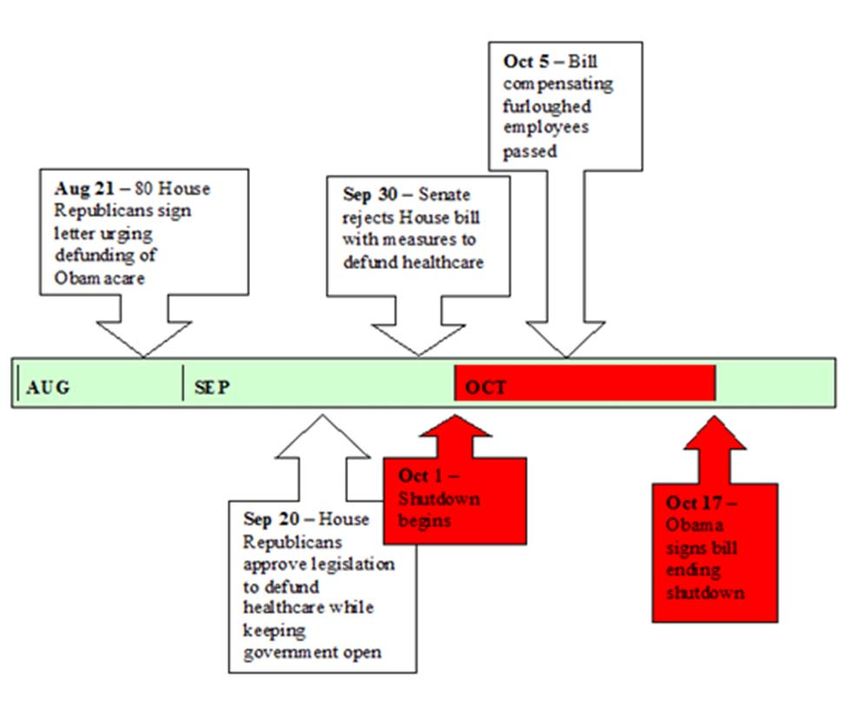
By showing a wide span of data before and after the shutdown, Figure 2 provides
strong evidence of the adequacy of the control group and the effectiveness of using
average daily spending as the normalization. Figure 2 shows that the employees not
subject to the shutdown have nearly identical movement in spending except during
the weeks surrounding the shutdown. Thus the controls appear effective at captur-
ing aggregate shocks, seasonality, payday interactions, etc. In particular, note the
regular, biweekly pattern of fluctuations in spending. It arises largely from the tim-
ing of spending following receipt of the bi-weekly paychecks. There are also subtler
beginning-of-month effects—also related to timing of spending. In subsequent figures
we use a narrower window to highlight the effects of the shutdown.
Gelman et al. (2014) shows that much of the sensitivity of spending to receipt of
paycheck, like that seen in Figure 2, arises from reasonable choices of individuals to
time recurring payments—such as mortgage payments, rent, or other recurring bills—
immediately after receipt of paychecks. Figure 2 makes clear that the control group
does a good job of capturing this feature of the data and therefore eliminating ordinary
paycheck effects from the analysis. The first vertical line in Figure 2 indicates the
week in which employees affected by the shutdown were paid roughly 40% less than
their average paycheck. There is a large gap between the treatment and control group
during this week. Similarly, the second vertical line indicates the week of the first
paycheck after the shutdown. The rebound in spending is discernable for two weeks.
The figure thus demonstrates that the control group represents a valid counterfactual
for spending that occurred in the absence of the government shutdown.
4.3 Liquidity Before the Shutdown
To understand how affected employees responded to the shutdown, it is useful to
examine first how they and others like them managed their liquid assets prior to the
shock. Analysis of liquid asset balances before the shutdown shows that, while some
workers were well buffered, many were ill-prepared to use liquid assets to smooth even
a brief income shock.
We define liquid assets as the balance on all checking and savings accounts. The
11measure of liquidity is based on daily snapshots of account balances. Hence, they are
measures of the stock of liquid assets independent from the transactional data used
to measure spending and income. Having such high-frequency data makes it possible
to observe distinctive, new evidence on liquidity and how it interacts with shocks.
Figure 3 shows median liquidity over the pay-cycle, by terciles of the distribution of
liquidity. Liquidity is expressed as a ratio of checking and savings account balances
to average daily total spending. The results are for the period prior to the shutdown
and aggregate over both treatment and control groups.10,11
While the optimal level of liquidity is not clear, the figure shows the top third
of the liquidity distribution is well-positioned to handle the income shock due to the
shutdown. The median of this group could maintain more than a month of average
spending with their checking and savings account balances, even in the days just
before their paycheck arrives.
The lower two-thirds of the liquidity distribution has a substantially smaller cush-
ion. Over the entire pay-cycle, the middle tercile has median liquid assets equal to
7.9 days of average spending. Liquidity drops to only 5 days of average spending in
the days just before their paycheck arrives. Thus, even in the middle of the liquidity
distribution many would be hard pressed to use liquid savings to smooth a tempo-
rary loss of 4 days pay. The bottom third of this population is especially ill-prepared.
Prior to the shutdown, the median of this group consistently arrives at payday with
precisely zero liquid balances. (Balances can be negative owing to overdrafts.) These
balance data thus reveal how, even among those with steady employment, large frac-
tions of consumers do not have the liquid assets to absorb a large, but brief, shock to
income.
10
The distributions for treatment and control are similar. For example, in the control group the
median liquidity ratio for the first, second, and third, terciles of the liquidity distribution is, 2.9,
7.9, and 32.1, respectively. The analogous numbers for the treatment group are 3.3, 8.1, and 32.0.
11
Liquidity peaks two days after a payday. The balance data are based on funds available, so
liquidity should lag payday according to the banks funds-availability policy. There is at least one-
day lag built into the data because the balances are scraped during the day, so will reflect a paycheck
posted the previous day. Appendix Figure A4 shows that the two-day delay in the peak of liquidity
is due to funds availability, not delays in posting based on interactions of day of payday and delays
in posting of transactions over the week-end. (As discussed in the Appendix, even within the
government bi-weekly pay schedule, there is some heterogeneity in day of week of the payday.)
Additionally, liquidity is, of course, net of inflows and outflows. Recurring payments made just after
the receipt of paycheck will therefore lead daily balances to understate gross liquidity right after the
receipt of the paycheck.
125 Responses to the Shutdown
Having established that many (affected) workers had little liquidity prior to the shut-
down, we now examine how their income, and various form of spending responded
to the shutdown. Our method is to estimate the difference-in-difference, between
treatment and control, for various outcomes using the equation,
T T
βk × W eeki,k × Shuti + Γ0 Xi,t + i,t ,
X X
yi,t = δk × W eeki,k + (1)
k=1 k=1
where y represents the outcome variable (total spending, non-recurring spending, in-
come, debt, savings, etc.), i indexes individuals (i ∈ {1, ..., N }), and t indexes time
(t ∈ {1, ..., T }). W eeki,k is a complete set of indicator variables for each individual-
week in the sample, Shuti is a binary variable equal to 1 if individual i is in the treat-
ment group and 0 otherwise, and Xi,t represents controls to absorb the predictable
variation arising from bi-weekly pay week patterns.12 The βk coefficients capture the
average weekly difference in the outcome variables of the treatment group relative
to the control group. Standard errors in all regression analyses are clustered at the
individual level and adjusted for conditional heteroskedasticity.
5.1 Paycheck Income and Total Spending
We begin with an examination of how income, as measured in these data, was affected
by the shutdown. External reports indicate that the paycheck income of affected
employees should have dropped by 40% on average. The analysis of paycheck income
here can thus be viewed, in part, as testing the ability of these data to accurately
measure that drop. Once that ability is confirmed, we move to an evaluation of the
spending responses.
Recall that we normalize each variable of interest, measured at the individual level,
by the individual’s average daily spending computed over the entire sample period.
The unit of analysis in our figures is therefore days of average spending. Figure 4
plots the estimated βk from equation (1) where y is normalized paycheck income.
12
Specifically, Xi,t contains dummies for paycheck week, treatment, and their interaction. This
specification allows the response of treatment and control to ordinary paychecks to differ. These
controls are only necessary in the estimates for paycheck income.
13We plot three months before and after the government shutdown to highlight the
effect of the event. The first vertical line (dashed-blue) represents the week that the
shutdown began and the second vertical line (solid-red) represents the week in which
pay dropped due to the shutdown, and the third when pay was restored.
Panel A of Figure 4 shows, as expected, a drop in income equal to approximately
4 days of average daily total spending during the first paycheck period after the
shutdown.13 This drop quickly recovers during the first paycheck period after the
shutdown ends, as all users are reimbursed for their lost income. Some users received
their reimbursement paychecks earlier than usual, so the recovery is spread across
two weeks. The results confirm that the treatment group is indeed subject to the
temporary loss and subsequent recovery of income that was caused by the government
shutdown, and that the account data allow an accurate measure of those income
changes.
Panel B of Figure 4 plots the results on total spending, showing the estimated βk
where y is normalized total spending. On average, total spending drops by about 2
days of spending in the week the reduced paycheck was received. Hence, the drop in
spending upon impact is about half the drop in income. That implies a propensity to
spend of about one-half—much higher than most theories would predict for a drop of
income that was widely expected to be made up in the relatively near future. In the
inter-paycheck week, spending is about normal. In the second week after the paycheck
affected by the shutdown, spending rebounds with the recovery spread mainly over
that week and the next one.
To ease interpretation we convert the patterns observed in Figure 4 into an esti-
mate of the marginal propensity to spend (which we call the MPC as conventional).
Let τ be the week of the reduced paycheck during the shutdown. The variable si,τ −k
denotes total spending for individual i in the k weeks surrounding that week. To
estimate the MPC, we consider the relationship,
si,τ −k = αk + βkM P C (P aychecki,τ − P aychecki,τ −2 ) + i,τ −k , (2)
13
The biweekly paychecks dropped by 40 percent on average. For the sample, paycheck income
is roughly 70 percent of total spending on average because there are other sources of income. So a
drop of paycheck income corresponding to 4 days of average daily spending is about what one would
expect (4 days ≈ 0.4 × 0.7 × 14 days).
14where (P aychecki,τ − P aychecki,τ −2 ) is the change in paycheck income. Both si,τ −k
and P aychecki,τ are normalized by individual-level average daily spending as dis-
cussed above. We present estimates for the one and two week anticipation of the
drop in pay (k = 1 and k = 2), the contemporaneous MPC (k = 0), and one lagged
MPC (k = −1). We do not consider further lags because the effect of the lost pay is
confounded by the effect of the reimbursed pay beginning at time τ + 2.
There are multiple approaches to estimating equation (2). The explanatory vari-
able is the change in paycheck. We are interested in isolating the effect on spending
due to the exogenous drop in pay for employees affected by the shutdown. While in
concept this treatment represents a 40 percent drop in income for the affected em-
ployees and 0 for the controls, there are idiosyncratic movements in income unrelated
to the shutdown. First, not all employees affected by the shutdown had exactly a 40
percent drop in pay because of differences in work schedule or overtime during the
pay period. Second, there are idiosyncratic movements in pay in the control group.
Therefore, to estimate the effect of the shutdown using equation (2) we use an instru-
mental variables approach where the instrument is a dummy variable Shuti . The IV
estimate is numerically equivalent to the difference-in-difference estimator.14
Table 3 shows the estimates of the MPC. These estimates confirm that the total
spending of government employees reacted strongly to their drop in income and that
this reaction was focused largely during the week that their reduced paycheck arrived.
The estimate of the average MPC is 0.58 in this week, with much smaller coefficients
in the two weeks just prior. Thus, at the margin, about half of the lost income was
reflected in reduced spending.
14
Estimating equation (2) by least squares should produce a substantially attenuated estimate
relative to the true effect of the shutdown if there is idiosyncratic movement in income among the
control group, some of which results in changes in spending. In addition, if the behavioral response
to the shutdown differs across individuals in ways related to variation in the change in paycheck
caused by the shutdown (e.g., because employees with overtime pay might have systematically
different MPCs), the difference between the OLS and IV estimates would also reflect treatment
heterogeneity. This heterogeneity could lead the OLS estimate to be either larger or smaller than
the IV estimate, depending on the correlation between of the size of the shutdown-induced shock
and the MPC. The OLS estimate of the MPC for the week the reduced paycheck arrived is 0.123,
with a standard error of 0.004.
155.2 Spending and Payments by Type
Analyzing different categories of spending offers further insight into the response of
these users to the income drop. We separate spending into non-recurring and recurring
components. Recurring spending is identified using patterns in both the amount
and transaction description of each individual transaction.15 It identifies spending
that, due to its regularity, is very likely to be a committed form of expenditure
(see Grossman and Laroque (1990), Chetty and Szeidl (2007), and Postlewaite, et
al. (2008)). Non-recurring spending is total spending minus recurring spending.
These measures thus use the amount and timing of spending rather than an a priori
categorization based on goods and services. This approach to categorization is made
possible by the distinctive features of the data infrastructure.
Figure 5 presents estimates of the βk from equation (1) where the outcome variable
y takes on different spending, payment, or transfer categories. For each graph, the
data are normalized by individual-level averages for the series being plotted. In the
top two panels we can compare the normalized response of recurring and non-recurring
spending and see important heterogeneity in the spending response by category. The
results on total spending (Figure 4) showed an asymmetry in the spending response
before and after the income shock; total spending dropped roughly by 2 days of
average spending during the three weeks after the shutdown began and only rose by
1.6 days of average spending during the three weeks after the shutdown ended. The
reaction of recurring spending drives much of that asymmetry; it dropped by 2.6
days of average recurring spending and rose only by 0.84 days once the lost income
was recovered. Non-recurring spending exhibits the opposite tendency: it dropped
by 1.8 days of average non-recurring spending and rose by 2.0 days. Thus, recurring
spending drops more and does not recover as strongly as non-recurring spending.
To better understand this pattern of recurring expenditure and its significance we
focus on a particular, and especially important, type of recurring spending—mortgage
payments. Panel C of Figure 5 shows that, while the mortgage spending data is noisier
15
We identify recurring spending using two techniques. First, we define a payment as recurring if
it takes the same amount at a regular periodicity. This definition captures payments such as rent
or mortgages. Second, we also use transaction fields to identify payments that are made to the
same payee at regular intervals, but not necessarily in the same amount. This definition captures
payments such as phone or utility bills that are recurring, but in different amounts. See appendix
for further details. Gelman et al. (2014) uses only the first technique to define recurring payments.
16than the other categories, there is a significant drop during the shutdown and this
decline fully recovers in the weeks when the employees’ missing income was repaid. In
this way, we see that some users manage the shock by putting off mortgage payments
until the shutdown ends. Indeed, many of those affected by the shutdown changed
from paying their mortgage early in October to later in the month as shown in Figure
6. The irregular pattern of payment week of mortgage reflects interaction of the bi-
weekly paycheck schedule with the calendar month. The key finding of this figure is
that the deficit in payments of the treatment group in the second week of October is
largely offset by the surplus of payments in the last two weeks of October.
Panel D of Figure 5 shows the response of account transfers to the income shock.16
During the paycheck week affected by the shutdown, transfers fell and rebounded
when the pay was reimbursed two weeks later. This finding implies a margin of
adjustment, reducing transfers out of linked accounts, during the affected week. One
might have expected the opposite, i.e., an inflow of liquidity from unlinked asset
accounts to make up for the shortfall in pay. That kind of buffering is not present on
average in these data.
Similar behavior is seen in the management of credit card accounts. Another
relatively low-cost way to manage cash holdings is to postpone credit card balance
payments. Panel E of Figure 5 shows there was a sharp drop in credit card balance
payments during the shutdown, which was reversed once the shutdown ended. For
users who pay their bill early, this is an easy and cost-free way to finance their current
spending. Even if users are using revolving debt, the cost of putting off payments
may be small if they pay off the balance right away after the shutdown ends. We
examine credit card balances in greater detail in the next section.
Indeed, as we see in Panel F of Figure 5, there was no average reaction of credit
card spending to the shutdown. Thus, we find no evidence that affected employ-
ees sought to fund more of their expenditure with credit cards but instead floated,
temporarily, more of their prior expenditure by postponing payments on credit card
balances. Affected individuals who had ample capacity to borrow in order to smooth
16
These are transactions explicitly labeled as “transfer,” etc. For linked accounts, they should net
out (though it is possible that a transfer into and out of linked accounts could show up in different
weeks). Hence, these transfers are (largely) to and from accounts (such as money market funds)
that are not linked.
17spending, by charging extra amounts to credit cards, had other means of smoothing,
e.g., liquid checking account balances or the postponement of mortgage payments.
On the other hand, those who one might think would use credit cards for smoothing
spending because they had little cash on hand did not—either because they were
constrained by credit limits or preferred to avoid additional borrowing. In the next
section we will examine the consequences for credit card balances of these postponed
balance payments, and later probe the heterogeneous responses of individuals by their
level of liquidity.
This analysis of different categories of spending reveals that users affected by the
shutdown reduce spending more heavily on recurring spending and payments com-
pared to non-recurring spending. It is important to note that this behavior appears
to represent, in many cases, a temporal shifting of payments and neither a drop in
eventual spending over a longer horizon or a proportionate drop in contemporaneous
consumption. These results thus provide evidence of the instruments that individuals
use to smooth temporary shocks to income that has not been documented before.
The drop in non-recurring spending shows, however, that this method of cash man-
agement is not perfect; it does not entirely smooth spending categories that better
reflect consumption.
Spending could have fallen in part because employees stayed home and engaged
in home production instead of frequenting establishments that they encounter during
their work-day. Recall, however, that many employees affected by the shutdown were
not, in fact, furloughed. They worked but did not get paid for that work on the
regular schedule. In addition, Figure 7 shows that categories of expenditure that are
quite close to consumption, such as a fast food and coffee shops spending index, show
a sharp drop during the week starting October 10 when employees were out of work.
Given that a cup of coffee or fast food meal is non-durable, one would not expect
these categories to rebound after the shutdown. Yet, there is significant rebound after
the shutdown. We interpret this spending as resulting from going for coffee, etc., with
co-workers after the shutdown, perhaps to trade war stories.17 Hence, in a sense, a
cup of coffee is not entering the utility function as an additively separate non-durable.
17
Interestingly, the rebound is highest for the most liquid individuals (figure not reported) who
are also higher income. This finding supports our notion that the rebound in coffee shop and fast
food arises from post-shutdown socializing.
185.3 Response of Liquid Assets
For users who have built up a liquid asset buffer, they may draw down on these re-
serves to help smooth income shocks. Figure 8 shows the estimated βk from equation
(1) where yi,t is the weekly average liquid balance normalized by its individual-level av-
erage (Panel A) or normalized by individual-level average daily total spending (Panel
B). Because of the heterogeneity in balances, normalizing by average liquid balances
leads to more precise results. Normalizing by total spending is less precise but al-
lows for a more meaningful interpretation because it is in the same units as Figure 4.
Consistent with the spending analysis, relative savings for the treatment group rises
in anticipation of the temporary drop in paycheck income. There is a steep drop in
the average balance the week of the lower paycheck as a result of the shutdown. The
drop in liquidity is, however, substantially attenuated relative to the drop in income
because of the drop in payments that is documented in the previous section. The
recovery of the lost income causes a large spike in the balances, which is mostly run
off during the following weeks. Figure 8B shows that liquid balances fell by around
2 day of average daily total spending. Therefore, on average, users reduced spending
by about 2 days and drew down about 2 days of liquidity to fund their consumption
when faced with a roughly 4 days drop in income. These need not add up because of
transfers from non-linked accounts and because of changes in credit card payments,
though they do add up roughly at the aggregate level. In the next section, we explore
the heterogeneity in responses as a function of liquid asset positions where specific
groups of individuals do use other margins of adjustment than liquid assets.
6 Liquidity and the Heterogeneity in Response to
the Income Shock
The preceding results capture average effects of the shutdown. There are important
reasons to think, however, that different employees will react differently to this income
shock, depending on their financial circumstances. Although all may have a desire
to smooth their spending in response to a temporary shock, some may not have the
means to do so.
19In this section we examine the heterogeneity in the response along the critical
dimension of liquidity. For those with substantial liquid balances relative to typical
spending, it should be relatively easy to smooth through the shutdown. Section 4
showed, however, that many workers in these data have little liquidity, especially in
the days just before their regular paycheck arrives. For those (barely) living paycheck-
to-paycheck, even this brief drop in income may pose significant difficulties.
We investigate the impact of the shutdown for those with varying levels of liquidity
by first further quantifying the buffer of liquid assets that different groups of workers
had. Second, we return to each of the spending categories examined above and
compare how different segments of the liquidity distribution responded to the income
shock. Last, we study how the precise timing of the shock, relative to credit card due
dates, influenced credit card balances coming out of the shutdown.
6.1 Liquidity and Spending
As before, we define the liquidity ratio for each user as the average daily balance of
checking and savings accounts to the user’s average daily spending until the govern-
ment shutdown started on October 1, 2013 and then divide users into three terciles.
Table 4 shows characteristics of each tercile. Users in the highest tercile have on aver-
age 54 days of daily spending on hand while the lowest tercile only has about 3 days.
This indicates that a drop in income equivalent to 4 days of spending should have
significantly greater effects for the lowest tercile compared with the highest tercile.
Figure 9 plots the estimates of βk s from equation (1), for various forms of spending,
by terciles of liquidity. The results are consistent with liquidity playing a major role in
the lack of smoothing. Users with little buffer of liquid savings are more likely to have
problems making large and recurring payments such as rent, mortgage, and credit
card balances. In terms of average daily expenditure, spending for these recurring
payments drops the most for low liquidity users. In contrast, the drop in non-recurring
spending is similar across all liquidity groups. Like those with more liquidity, however,
low liquidity users refrained from using additional credit card spending to smooth the
income drop.
206.2 Liquidity and Credit Debt
The preceding results indicate that the sharp declines in recurring spending (espe-
cially mortgages) and credit card balance payments induced by the shutdown were
particularly important strategies for those with lower levels of liquidity. The gran-
ularity of the data shows, however, that fine differences in timing are consequential
when liquidity levels are so low.
To examine how individuals manage credit card payments and balances, we carry
out the analysis at the level of the individual credit card account, rather than aggre-
gating across accounts as in the previous section. The account-level analysis allows us
to examine the role of payment due dates in the response to the shutdown. These due
dates may represent significant requirements for liquidity. That they are staggered
and unlikely to be systematically related to the timing of the shutdown provides an-
other means for identifying behavioral responses that exploits the high resolution of
the data infrastructure.
In this analysis, however, attention is restricted to the accounts of “revolvers.”
We focus, that is, on accounts held by those who, at some point during the study
period (including the period of the shutdown), incurred interest charges on at least
one of their credit cards, indicating that they carried some revolving credit card debt.
This represents 63% of the treatment group and 63% of controls; and 70% of these
workers fall in the lower two-thirds of the liquidity distribution. The complement
of the revolver group is the “transactors.” Members of this group routinely pay
their entire credit card balance, and have a distinct monthly pattern of balances that
reflects their credit card spending over the billing cycle and regular payment of the
balance at the end of the cycle. Only 44% of transactors fall in the lower two thirds
of the liquidity distribution. Including transactors would obscure the results for those
who carry credit card debt.18
Figure 10 shows the response of credit card balances, at the account level, to the
loss of income due to the shutdown. The estimates again present the difference-in-
difference between accounts held by revolvers in the treatment group and those held
18
We investigated those who shifted from being transactors to revolvers at the time of the shut-
down. This group was so small (17%) that it did not yield interesting results. Given that transactors
tend to have high liquidity (15.9 median ratio vs 7.7 for revolvers), the lack of such transitions is
not surprising.
21by revolvers in the control group. These estimates are specified in terms of days
since the account’s August 2013 statement date instead of calendar time in order
to show the effect of statement due dates. In Figure 10, Days 0 through 30 on the
horizontal axis correspond to payment due dates in late August or in September 2013.
(Payments are due typically 25 days after the statement date.) The different panels of
Figure 10 show alternative cuts of the data that we will explain next. Focus, however,
on the first 25 days since the August statement date, i.e., due dates that occur in
advance of the shutdown. Regardless of cut on the data, the difference-in-difference
between treatment and control is essentially zero.
Panels A and B divide the sample of accounts into two groups based on the credit
card statement date and, in particular, whether the statement date places them “at
risk” for having to make a payment during the government shutdown. Panel A
shows the accounts with statement dates on September 16-30, 2013. Panel B shows
accounts that have statement dates on September 1-15. For those in the treatment
group, the accounts with September 16-30 due dates (Panel A) are at risk. Based on
our analysis of liquidity over the paycheck cycle (Figure 3) it is likely that the mid-
October paycheck that is diminished by the shutdown would have been a primary
source of liquidity for making the payment on these accounts that come due during
that pay period. Indeed, Panel A reveals this effect. Control and treatment accounts
start to diverge about a week to 10 days into the October billing cycle (days 35-37).
By the time the November statement arrives (days 58-60), a significant gap emerges;
relative to controls, treatment account balances are now significantly above average.
They return to average in a month, presumably as affected workers use retroactive
pay to make balance payments. Panel B, those who made their payments before the
shutdown, shows no such effect (the hump starting at day 30 is prior to the shutdown
and is not statistically significant.)
The high-resolution analysis made possible with the data infrastructure reveals
that, when liquidity is so low, small differences in timing can matter. Workers whose
usual credit card payment date fell before the shutdown adjusted on other margins;
their balances did not rise. For others, the shutdown hit just as they would have
normally made their credit card payment; they deferred credit card payments and
their balances were elevated for a billing cycle or two before returning to normal
22levels.
These findings for credit cards reinforce the findings for mortgage payments found
in the previous section and Figure 6. For those who typically made payments on
mortgages early in the month, that is, prior to the receiving the paycheck reduced
by the shutdown, there is little effect of the shutdown on mortgage payments. For
those who make payments in the second half of the month, they can and often did
postpone the mortgage payments as a way to respond to the shock to liquidity.
7 Conclusion
Living paycheck-to-paycheck lets workers consume at higher levels, but would seem
to leave them quite vulnerable to income shocks. The results of this paper reveal
how workers use financial assets and markets, sometimes in unconventional ways, to
reduce that vulnerability and adjust to shocks when they do occur. The findings
indicate that to the extent a large but brief shock to income is a primary risk, a lack
of liquid assets as a buffer is not necessarily a sign of myopia or unfounded optimism.
Rather, the reactions to the 2013 government shutdown studied in this paper indicate
that workers can defer debt payments and thus maintain consumption (at low cost)
despite limited liquid assets. They may face higher costs to access less liquid assets.
Such illiquidity may be optimal even if it leads to short- or medium-run liquidity
constraints (see Kaplan and Violante 2013). This paper shows that the majority of
households have such liquidity constraints, yet they have mechanisms for coping with
shocks to income so as to mitigate the consequences of such illiquidity.
This paper provides direct evidence on the importance of deferring debt payments,
especially mortgages, as an instrument for consumption smoothing. Mortgages func-
tion for many as a primary line of credit. By deferring a mortgage payment, they can
continue to consume housing, while waiting for an income loss to be recovered. For
changing the timing of mortgage payments within the month due, there is no cost.
As discussed above, that is the pattern for the bulk of deferred mortgage payments.
Moreover, the cost of paying one month late can also be low. Many mortgages allow
a grace period after the official due date, in which not even late charges are incurred,
or charge a fee that is 4-6 percent of the late payment. Being late by a month adds
23You can also read