HURRICANES AND GLOBAL WARMING - Results from Downscaling IPCC AR4 Simulations
←
→
Page content transcription
If your browser does not render page correctly, please read the page content below
HURRICANES AND GLOBAL
                     WARMING
              Results from Downscaling IPCC AR4 Simulations
                                  BY   KERRY EMANUEL, R AGOTH SUNDARARAJAN, AND JOHN WILLIAMS

             A new technique for deriving hurricane climatologies from global data, applied to climate
             models, indicates that global warming should reduce the global frequency of hurricanes,
                              though their intensity may increase in some locations.

      T
           ropical cyclones account for the majority of                   relatively short length of tropical storm records. In
           natural catastrophic losses in the developed                   the North Atlantic region, dense ship tracks, islands,
           world and, next to floods, are the leading cause               and the relatively small size of the basin have led to
      of death and injury among natural disasters affecting               the creation of an official archive extending back to
      developing countries (UNDP/BCPR 2004). It is thus                   1851 (Jarvinen et al. 1984; Landsea et al. 2004), but the
      of some interest to understand how their behavior                   detection rate prior to the satellite era remains con-
      is affected by climate change, whether natural or                   troversial (Landsea 2007). Routine aircraft reconnais-
      anthropogenic.                                                      sance of tropical cyclones began shortly after WWII
         A range of techniques has been brought to bear on                in the North Atlantic and western North Pacific
      this question. The most straightforward approach is                 regions, and while it continues to this day over the
      to quantify the response of tropical cyclone activity               Atlantic, it was terminated in 1987 over the western
      to past climate change using historical climate and                 North Pacific. These missions undoubtedly improved
      storm records, but this approach is limited by the                  the detection rate, though it is possible that some
                                                                          storms were still missed. In the active tropical cyclone
                                                                          belts of the eastern North Pacific, and in virtually
AFFILIATIONS: E MANUEL , S UNDARARAJAN ,
                                       AND WILLIAMS —Program
                                                                          all of the Southern Hemisphere, high detection rates
in Atmospheres, Oceans, and Climate, Massachusetts Institute of
                                                                          were not achieved until about 1970, when satellites
Technology, Cambridge, Massachusetts
CORRESPONDING AUTHOR: Kerry Emanuel, Room 54-1620,
                                                                          covered a sufficiently high portion of the globe.
MIT, 77 Massachusetts Ave., Cambridge, MA 02139                               This relatively short and flawed record of tropical
E-mail: emanuel@texmex.mit.edu                                            cyclone activity has nevertheless led to the detec-
                                                                          tion of significant climatic influences on tropical
The abstract for this article can be found in this issue, following the
table of contents.
                                                                          cyclone activity, most prominently, the influence of
DOI:10.1175/BAMS-89-3-347                                                 El Niño–Southern Oscillation (ENSO) on storms in
                                                                          the North Atlantic (Gray 1984; Bove et al. 1998; Pielke
In final form 29 October 2007
©2008 American Meteorological Society                                     and Landsea 1999; Elsner et al. 2001) and western
                                                                          North Pacific (Chan 1985). Variations on time scales

      AMERICAN METEOROLOGICAL SOCIETY                                                                         MARCH 2008          | 347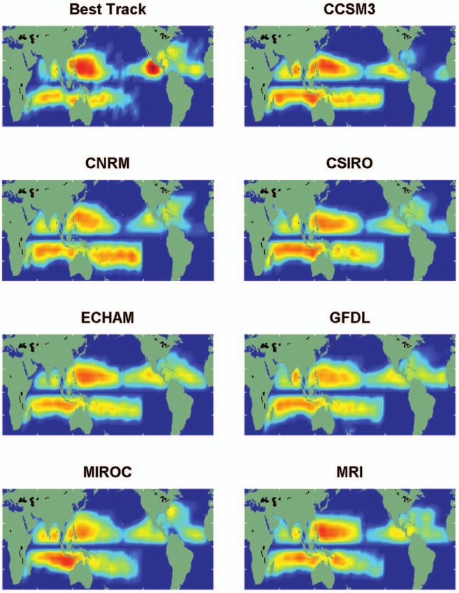
of several decades have also been discussed, with early    to the output of a global climate model by Emanuel
    work attributing such variations to natural climate        (1987) showed a significant increase of potential
    f luctuations, such as the Atlantic Multi-Decadal          intensity in a double-CO2 climate.
    Oscillation (Goldenberg et al. 2001) and the Pacific           The horizontal resolution of the current gen-
    decadal oscillation (Chan and Shi 1996). The subse-        eration of global climate models is insufficient to
    quent attribution of decadal variability and trends to     simulate the complex inner core of intense tropical
    radiatively forced climate change by Emanuel (2005a)       cyclones; the highest resolution achieved to date has
    and Webster et al. (2005) led to a vigorous debate and     a horizontal grid spacing of 20 km (Oouchi et al.
    reexamination of the quality of the tropical cyclone       2006), whereas numerical convergence tests using
    record (Emanuel 2005b; Landsea 2005; Chan 2006;            mesoscale models suggest that grid spacing of the
    Landsea et al. 2006; Chang and Guo 2007; Kossin            order of 1 km may be required (Chen et al. 2007).
    et al. 2007; Landsea 2007), while the sources of the       Nevertheless, many global models produce reasonable
    trends and variability continue to be debated (Curry       facsimiles of tropical cyclones, and many studies have
    et al. 2006; Hoyos et al. 2006; Santer et al. 2006;        documented the effects of climate change on these
    Emanuel 2007; Mann et al. 2007).                           simulated disturbances (Bengtsson et al. 1996; Sugi
        Another approach to the problem is to extend the       et al. 2002; Oouchi et al. 2006; Yoshimura et al. 2006;
    tropical cyclone record back into prehistory using         Bengtsson et al. 2007). While there is a wide varia-
    proxies for storm activity detected in the geological      tion in the results of these studies, there is a tendency
    record, an endeavor known as paleotempestology.            toward decreasing frequency and increasing intensity
    Proxies used so far include storm-driven overwash          and precipitation of tropical cyclones as the climate
    deposits in near-shore lakes and marshes (Liu              warms (Bengtsson et al. 2007).
    and Fearn 1993; Donnelly and Woodruff 2007),                   Another way to use global models to assess future
    oxygen isotopic anomalies recorded in speleothems          tropical cyclone activity is to identify changes in
    (Malmquist 1997; Frappier et al. 2007) and tree rings      large-scale environmental factors that are known to
    (Miller et al. 2006), and storm-driven beach deposits      affect storm activity. For example, a recent study by
    (Nott 2003). Reconstructions of coastal tropical cyclone   Vecchi and Soden (2007) showed that a consensus of
    activity, some of which now extend over thousands of       global climate models predicts increasing wind shear
    years, are beginning to reveal patterns of variability     over the North Atlantic with warming. This would
    on decadal-to-centennial time scales (Liu and Fearn        tend to inhibit tropical cyclone activity, all other
    1993; Donnelly and Woodruff 2007). At present, such        things being equal.
    techniques are limited to coastal regions.                     The limitations of the low resolution of the GCMs
        Basic theory has been used to predict the depen-       can be circumvented by embedding in them high-
    dence of hurricane intensity (as measured by maxi-         resolution regional models, an approach that was
    mum wind speeds or minimum surface pressures)              pioneered by Knutson et al. (1998) and Knutson and
    on climate (Emanuel 1987), but there is at present         Tuleya (2004). In this method, the GCM supplies
    very little theoretical guidance pertaining to the         boundary and initial conditions to the regional
    frequency or duration of events. Potential intensity       model, which produces its own climatology of tropical
    theory (Emanuel 1986; Bister and Emanuel 1998) has         cyclones. This approach has been applied so far to
    been widely interpreted as predicting a particular         idealized climate change scenarios (Knutson et al.
    dependence of tropical cyclone wind speeds on sea          1998; Knutson and Tuleya 2004), to the climate of the
    surface temperature (Landsea 2005), though in reality      late twentieth century (Knutson et al. 2007), and most
    the predicted dependence is on the air–sea thermo-         recently to future climates affected by global warming
    dynamic disequilibrium and lower-stratospheric             (T. Knutson 2007, personal communication). This last
    temperature; the former of which can be shown to           study drove a regional model of the tropical North
    depend mostly on the net surface radiative flux and        Atlantic with a large-scale environment created by
    the average near-surface wind speed (Emanuel 2007).        averaging the output of 18 GCMs used for the most
    The robust 10% increase in summertime potential            recent report of the Intergovernmental Panel on
    intensity over the tropical North Atlantic since about     Climate Change (IPCC). The results are notable in
    1990 has been shown to depend on increasing net            that they predict decreasing storm activity over the
    surface radiative flux, cooling lower-stratospheric        North Atlantic, perhaps as a consequence of increased
    temperature, and decreasing surface wind speeds            vertical wind shear (Vecchi and Soden 2007), which
    (Emanuel 2007). Sea surface temperature is merely          is a circumstance widely recognized as inhibiting
    a cofactor. Application of potential intensity theory      cyclone activity.

348 |      MARCH 2008
These methods of downscaling are producing                  the “Coupled Hurricane Intensity Prediction
useful insights into the dependence of tropical cyclone        System” (“CHIPS”). The great advantage of this
activity on climate. At the present time, they are still       model is that it is phrased in angular momentum
limited in horizontal resolution, using grid spacing           coordinates, permitting a very high radial resolu-
of around 18 km, and they are expensive to conduct,            tion of the critical inner-core region using only
so that only a limited number of simulations can be            a limited number of radial nodes. This model
performed. For this reason, it is desirable to supplement      has been optimized over the past 8 yr to produce
these studies with methods that use simpler embedded           skillful, real-time hurricane intensity forecasts.
models that can be run a large number of times so as to        With one exception, noted in the “Genesis by
produce statistically robust estimates of the probability      random seeding” section below, we use the
distributions of storms in different climates.                 same version of this model that we use for real-
   The method pursued in this paper is an extension            time operational prediction of tropical cyclone
of that described by Emanuel et al. (2006) and                 intensity (Emanuel et al. 2004). Inputs to this
Emanuel (2006). Here we provide a brief overview of            model include the global model’s thermodynamic
the technique; the reader is referred to Emanuel et al.        state and wind shear derived from the global
(2006) and their online supplement for a complete              model’s wind statistics, as described in detail
description. Broadly, this approach uses both thermo-          in Emanuel et al. (2006). We also allow for vari-
dynamic and kinematic statistics derived from global           able midtropospheric temperature and relative
model or reanalysis gridded data to produce large              humidity, assigning the global model’s monthly
(~103 –10 4) numbers of synthetic tropical cyclones,           mean entropy of 600 hPa to the CHIP model’s
and these statistics are then used to characterize             midtropospheric entropy variable. While the
the tropical cyclone climatology of the given global           thermodynamic state also includes the global
climate. The synthetic tropical cyclones are produced          model’s predicted sea surface temperature, the
in the following three steps:                                  upper-ocean thermal structure (mixed layer
                                                               depth and sub–mixed layer thermal stratification)
1) Genesis. In previous implementations, tracks are            is taken from present climatology, owing to our
   initiated by randomly drawing from a space–time             lack of confidence in such quantities produced by
   genesis probability distribution based strictly on          current GCMs. The initialization of this model
   historical tropical cyclone data. In the “Genesis by        differs, however, from previous implementations,
   random seeding” section of this paper we describe           as described in “Genesis by random seeding.”
   a new technique based on random seeding, which              This intensity model is computationally effi-
   uses no historical data.                                    cient, making very large numbers of simulations
2) Tracks. We developed two independent track                  feasible.
   models, the first of which represents each track
   as a Markov chain driven by historical tropical          Aside from genesis, the method described above is
   cyclone track statistics as a function of location       independent of historical tropical cyclone data. To
   and time, while the second uses a “beta and              apply it to future climates as simulated using global
   advection” model to predict storm tracks using           models, it is highly desirable to relate the genesis
   only the large-scale background wind fields and          probability distribution to the actual climate state,
   a correction to account for drift induced by the         rather than to rely on historical distributions. A new
   storm’s advection of the planetary vorticity field.      technique for doing this is described in the following
   Here we employ the second method, because                section, and tests of the technique against observed
   we wish to predict tracks in future climates as          spatial, seasonal, and interannual variability are
   well as the present. The beta-and-advection              presented therein. This is followed by an applica-
   model uses synthetic wind time series of 850 and         tion to future climates simulated by IPCC Fourth
   250 hPa, represented as Fourier series of random         Assessment Report (AR4) models, as described in
   phase constrained to have the monthly means,             the “Application to global climate models” section,
   variances, and covariances calculated using daily        and a discussion of the results thereafter. A summary
   data from reanalyses or global models, and to            concludes the paper.
   have a geostrophic turbulence power-law distri-
   bution of kinetic energy.                                GENESIS BY RANDOM SEEDING. In the
3) Intensity. The wind field of each storm is predicted     traditional application of the synthetic track tech-
   using a deterministic, coupled air–sea model,            nique, storms are initiated at points drawn from a

AMERICAN METEOROLOGICAL SOCIETY                                                               MARCH 2008         | 349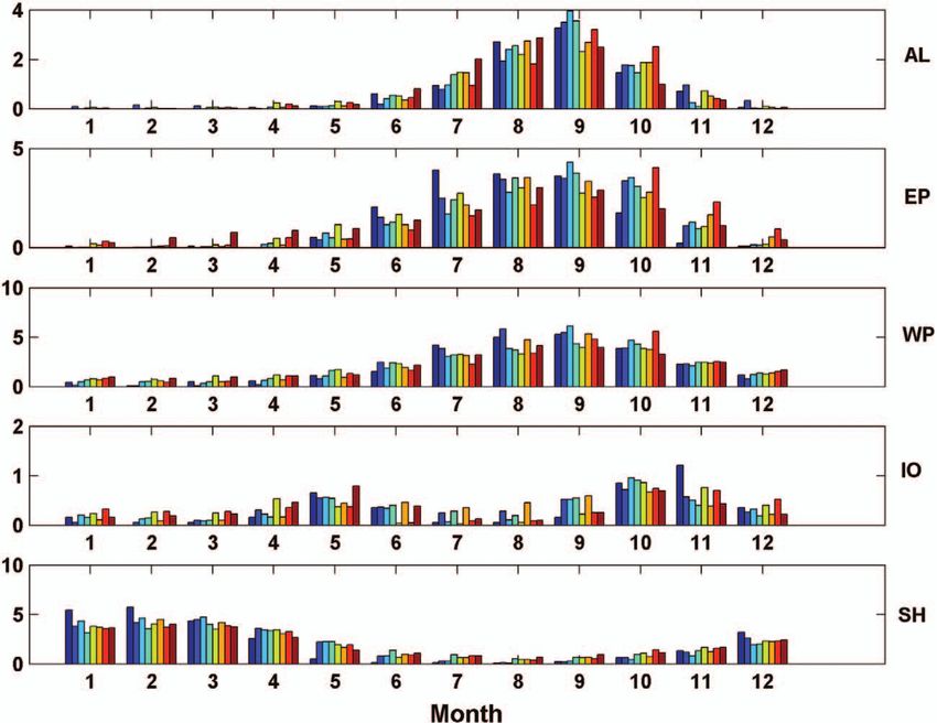
historically based genesis probability density func-      eterization is optimum for determining the survival
    tion, and, in the intensity model, are initiated with a   in shear of seed disturbances whose initial intensities
    warm-core vortex with peak winds of 17 m s–1 (35 kt).     are only 12 m s–1. At the suggestion of an anonymous
    Because real tropical cyclones develop at places and      reviewer, we modified the shear parameterization in
    times that are favorable for genesis, most of the         CHIPS in order to make the weaker storms more sus-
    storms initialized at this amplitude develop to some      ceptible to shear. The CHIPS shear parameterization
    degree.                                                   (see Emanuel et al. 2006) has multiplicative factors
        As an alternative to this procedure, we initiate      involving the model’s nondimensional maximum
    tracks at points that are randomly distributed in         wind speed and convective updraft mass flux; here
    space and time, but with warm-core vortices that          we place lower bounds on these two quantities as they
    have peak wind speeds of only 12 m s–1 (25 kt) and        appear in the parameterization. This increases the
    almost no midlevel humidity anomaly in their cores;       susceptibility to shear of the weaker disturbances,
    this causes them to decay initially (Emanuel 1989).       while leaving shear effects on strong storms unaltered.
    These random “seeds” are planted everywhere and           These lower bounds were loosely adjusted to optimize
    at all times, regardless of latitude, SST, season, or     predictions of seasonal and interannual variability
    other factors, except that storms are not allowed to      of storms in the current climate. Implementing this
    form equatorward of 2° latitude. These seed vortices      adjustment made a small, but noticeable, improve-
    track according to the beta-and-advection model, and      ment in the statistics described below.
    their intensity is predicted in the usual way using the       Figures 1a,b compare the empirical genesis distri-
    CHIPS model. The seeds are not considered to form         bution, based on 2,000 events in each of five basins,1
    tropical cyclones unless they develop winds of at         to the observed distribution from 1690 best-track
    least 21 m s–1 (40 kt). In practice, the great majority   events, in both cases for storms that go on to attain
    of seeds fail to develop by this criterion, succumbing    peak winds of at least 45 kt. The synthetic technique
    to small potential intensity, large wind shear, or low    uses reanalysis data from 1980 to 2005, and the best-
    midtropospheric entropy, and decaying rapidly after       track genesis points are from the same period. For
    initiation.                                               the present purpose, genesis is defined for the syn-
        Notably absent from this technique is any account     thetic events as the first point at which the maximum
    of the statistics of potential initiating disturbances,   winds exceed 30 kt. In order not to mask regions of
    such as easterly waves, or the empirical role of          infrequent events, the charts plot the logarithm of
    large-scale, low-level vorticity in genesis (Gray 1979;   1 + the number of points per 2.5° latitude–longitude
    Emanuel and Nolan 2004; Camargo et al. 2007).             area, and the absolute rate of genesis of the synthetic
    Random seeding assumes, in essence, that the prob-        events has been calibrated to yield the correct global
    ability of a suitable initiating disturbance is uniform   frequency. The frequencies of best-track and synthetic
    in both space and time. As a variation on random          events are compared for each basin in Fig. 1c.
    seeding, we therefore experimented with weighting             In general, there are too few events in the Atlantic
    the probability of genesis by various functions of        and eastern North Pacific relative to the rest of the
    the low-level (850 hPa) vorticity. Slightly improved      world. The synthetic distribution is weighted too far
    results are obtained by weighting the genesis prob-       west in the main development region (MDR) of the
    ability by the product of the Coriolis parameter          Atlantic, between Africa and the Caribbean, and does
    and the 850-hPa relative vorticity, not allowing the      not have a secondary maximum of activity off the
    weighting factor to be negative. We shall refer to        U.S. southeast coast. The local genesis maximum in
    this as “vorticity weighting.” In no case was genesis     the Caribbean is well to the southeast of the observed
    observed when the local potential intensity was less      maximum. In the western North Pacific, the simu-
    than 40 m s–1; thus, to save computing time, we do        lated storms broadly have the correct distribution, but
    not seed over land or elsewhere when the potential        the genesis region extends too far east and is located
    intensity is less than this value.                        too far south in the South China Sea. In the Southern
        The CHIPS model uses a parameterization of the        Hemisphere, the synthetic distribution is not far from
    deleterious effect of environmental wind shear on         that observed, but there are too many genesis events
    tropical cyclones, developed empirically over years
    of refining the model’s real-time predictions of storm    1
                                                                  Here the basins are defined as the North Atlantic, the
    intensity. Real-time predictions are made only for            North Pacific east of 160°W, the North Pacific west of
    developed storms with maximum wind speeds of at               160°W, the northern Indian Ocean, and all of the Southern
    least 17 m s–1, so it is not clear that the same param-       Hemisphere.

350 |      MARCH 2008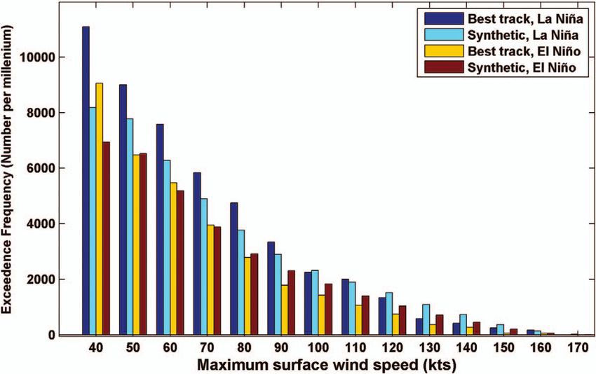
F IG . 1. Spatial distribution of genesis from (a) the
                                                          1980–2005 best-track data and (b) from 2,000 syn-
                                                          thetic events in each of five ocean basins, driven using
                                                          NCAR–NCEP reanalyses from 1980 to 2005. In all
                                                          cases, the spatial density is defined on a 2.5° grid,
                                                          and genesis is defined as the first point at which the
                                                          maximum wind speed exceeds 15 m s–1. The quantity
                                                          graphed is the logarithm of 1 + the genesis density, and
                                                          the color scale is the same in (a) and (b), increasing
                                                          from blue to red. (c) The observed annual frequency
                                                          is compared to the synthetic technique for each of
                                                          the five basins. (The South Atlantic is negligible in the
                                                          best-track and synthetic data.) There are 1,690 events
                                                          in the best-track data for this period.

in the region north of Madagascar. Note that there        North Pacific, where the synthetic technique also
are a few events in the South Atlantic; the predicted     predicts too few events (Fig. 1c), and in the north
frequency of events in that basin is about (7 yr) –1.     Indian Ocean, where too many storms are predicted.
   In comparing the synthetic to the observed spatial     In particular, the seasonal cycle in the eastern North
distributions shown in Fig. 1, bear in mind that          Pacific peaks too soon compared to observations,
some of the discrepancies may result from sampling,       and while the double peak in the north Indian Ocean
because there are more than 6 times the number of         is reproduced by the random seeding technique, its
synthetic events as there are best-track storms. Some     amplitude is too small, though the sample of observed
of the discrepancies may arise from not accounting        events is rather small in this case.
for the amplitude and frequency of potential initiating       Another test of the validity of the random seeding
disturbances in this technique; for example, in the       approach is its ability to distinguish between quiet
Atlantic, African easterly waves and quasi-baroclinic     and active periods. An example of particular interest
disturbances off the southeast U.S. coast may produce     is the well-known modulation of Atlantic tropical
genesis maxima that are not captured here.                cyclone activity by ENSO (Gray 1984; Bove et al.
   The annual cycle of genesis by month is shown          1998; Pielke and Landsea 1999; Elsner et al. 2001). In
in Fig. 2 for each of the five basins, and is compared    particular, El Niño is observed to suppress tropical
to the best-track data. To focus on the quality of the    cyclones in the Atlantic. Figure 3 compares the
annual-cycle per se, we have normalized the annual        exceedence frequencies of Atlantic tropical cyclones
count in each basin to be equal to the observed           as function of their lifetime peak wind speed as mea-
count for the period of 1980–2005 in this figure. To      sured during El Niño and La Niña years, as defined
estimate the closeness of fit to the data, we create      by Pielke and Landsea (1999).2 Because of the rela-
100 subsamples of the synthetic tracks, each with         tively small number of years in each category, we use
the same total number of tracks as contained in the
best-track data for the given period of time. The         2
                                                              For the present purpose, we lump “weak” and “strong” events
confidence limits shown in Fig. 2 represent limits            into a single category. The index for a particular winter
within which 90% of the subsamples are contained.             is held to be pertinent to the previous Atlantic hurricane
Genesis by random seeding produces an annual cycle            season, and we extended the Pielke and Landsea results by
very close to that of nature, although there are some         adding 2002 and 2004 to El Niño years, and 1998 and 2000
interesting discrepancies, particularly in the eastern        to La Niña years.

AMERICAN METEOROLOGICAL SOCIETY                                                                    MARCH 2008           | 351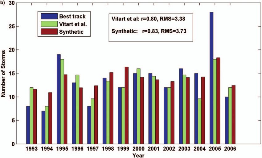
FIG . 2. Number of storms per month in each of the
                                                         five ocean basins, from best-track data (blue) and
                                                         from 2,000 synthetic events in each basin (red). The
                                                         annual total of the synthetic events is set equal to the
                                                         observed total in each basin in this case. The count
                                                         for the synthetic events represents the median of 100
                                                         random samples of 304 events for the Atlantic, 435
                                                         events for the eastern North Pacific, 801 events for
                                                         the western North Pacific, 126 events for the north
                                                         Indian Ocean, and 718 Southern Hemispheric events;
                                                         the error bars shows the limits within which 90% of
                                                         those samples lie.

                                                         years of the ENSO phase in question. As expected,
                                                         tropical cyclones of all intensities are less frequent
                                                         in El Niño years, though statistical significance is
                                                         not apparent through the whole range of intensities.
                                                         The difference between El Niño and La Niña is not
    the full reanalysis period of 1949–2004, and 2,000   quite as great among the synthetic events as is evi-
    synthetic events were run for each ENSO phase,       dent in the observations. To capture enough years
    using reanalysis data accumulated over only those    in each phase to lend better statistical significance

352 |     MARCH 2008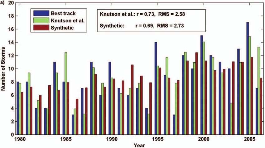
FIG. 3. Exceedence frequency distributions by intensity for North Atlantic storms for La Niña years
(dark and light blue bars), and El Niño years (yellow and red bars). In each pair of bars, the best-track
data pertain to the left member, and the synthetic data to the right. Data from the two phases of ENSO
during the period 1949–2004 are used for both the best-track and reanalysis data.

to the analysis, it was necessary to use almost the               Figure 4a compares the time series of the annual
entire 56-yr period of the National Centers for               frequency of North Atlantic events from 1980 to
Environmental Prediction–National Center for                  2006 with the observed annual frequency, based on
Atmospheric Research (NCEP–NCAR) reanalysis,                  best-track data, and with the annual frequency of
and it is well known that there are biases in the             events produced in a single simulation with a regional
reanalysis in the earlier part of this period.                model of the tropical Atlantic driven by boundary
    One further test that avoids the use of reanalysis        conditions supplied from the same NCEP–NCAR
data from early in the record is the comparison each          reanalysis as is used here, as reported in Knutson
year of the best-track data from 1980 to 2006 with            et al. (2007). Only storms that occurred in the months
synthetic storms produced using data from each                of August–October are included in this series, and
year of the reanalysis in this same time interval.3 We        the Knutson et al. results are based on their single
do this with some reservations, because the wind              model 2 run. The results here are statistically indistin-
covariance matrix used to synthesize winds for the            guishable from those of Knutson et al.; the synthetic
track model and for wind shear used as input to the           method used here explains about the same amount of
intensity model will be based on only 30 or 31 daily          the observed variance as that of Knutson et al., with
departures from the monthly averages. Nevertheless,           a slightly lower root-mean-square error and with a
if there is any skill in hindcasting tropical cyclone         mean trend of 0.19 yr–1, compared to the 0.21 yr–1
activity, it should be based on the deterministic part        in Knutson et al. Likewise, the power dissipation by
of the method, which involves the monthly mean                tropical cyclones in both the synthetic method and
reanalysis data, rather than the random components            the Knutson et al. method increases by about 200%
based on the covariances. To produce this time series,        over the period, with correlation coefficients between
we run 200 synthetic events for each year.                    the observed and simulated power dissipation time
                                                              series of around 0.7 in both cases.
3
    We thank T. Knutson and I. Held of National Oceanic and       Vitart et al. (2007) attempted to forecast and
    Atmospheric Administration/Geophysical Fluid Dynamics     reforecast Atlantic tropical cyclone activity over the
    Laboratory (NOAA/GFDL) for suggesting this.               period of 1993–2006, using the European Seasonal

AMERICAN METEOROLOGICAL SOCIETY                                                                   MARCH 2008          | 353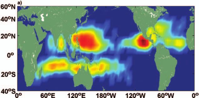
FIG. 4. Annual frequency of synthetic tropical cyclones in the North Atlantic (green bars) compared
    to best-track counts (blue bars) and to annual counts simulated by (a) Knutson et al. (2007) for the
    period of 1080–2006, and (b) Vitart et al. (2007) for the period of 1993–2006, shown in each case by
    red bars. The correlation coefficients (r) and root-mean-square errors (RMS) between the model and
    best-track storms are also indicated. The Knutson et al. simulations represent a single realization (their
    model 2), while the Vitart et al. count represents an ensemble median. Two hundred synthetic events
    were used each year. The data in (a) represent Aug–Oct storms only, while all events are included in
    (b). Note that subtropical events are included in the best-track data.

    to Interannual Prediction (EUROSIP) multimodel        is initialized either 40 or 41 times to produce an
    ensemble of coupled ocean–atmosphere models.          ensemble. The models are initialized on the first day
    This consists of three models, and each model         of each month and are used to forecast activity for

354 |      MARCH 2008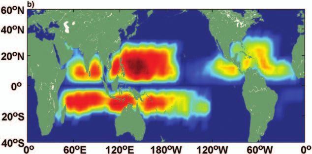
that month. Results were presented in which storms          Atlantic, the simulated increases are not in agree-
were reforecast for the period of 1993–2004, while          ment with the reanalysis of tropical cyclone power
real-time forecasts were used for 2005 and 2006. The        dissipation undertaken by Kossin et al. (2007), who
ensemble median number of storms in each year is            found that power dissipation decreased everywhere
compared with our synthetic storm count in Fig. 4b.         except in the North Atlantic, and, marginally, in the
As with the comparison with the Knutson et al. (2007)       western North Pacific.
results, our simulations are statistically very similar         The results presented in this section suggest that
to those of Vitart et al. Because those results are based   fairly realistic tropical cyclone climatologies can be
on one-month forecasts, any skill is attributable to        derived from global data that realistically represent
the skill in forecasting the monthly mean states            both the large-scale thermodynamic state of the
(including, possibly, the variances and covariances         tropical ocean and atmosphere and the large-scale
within those months) and not the details of day-to-         kinematic state, including day-to-day variations in
day fluctuations, whose predictability time scale is        winds through the depth of the troposphere. The
somewhat less than a month. Our results, together           genesis-by-natural-selection technique described
with those of Vitart et al. and Knutson et al., suggest     here also appears to give reasonable representations
that as much as half of the interannual variability of      of the spatial, annual, interannual, and interdecadal
Atlantic tropical cyclone activity can be attributed        variability of tropical cyclone activity, and is indepen-
to the characteristics of the monthly mean state of         dent of historical tropical cyclone data, allowing one
the atmosphere and ocean, and not to the details            to estimate storm activity in different climate states,
of high-frequency f luctuations, such as African            as described presently.
easterly waves. The residual root-mean-square error
of between three and four storms per year is also           APPLICATION TO GLOBAL CLIMATE
consistent with the results of Sabbatelli and Mann          MODELS. Application of this technique to global
(2007), who were able to attribute varying Atlantic         climate models is straightforward, as long as it is
storm counts to changing sea surface temperature            possible to derive the same kinematic and thermo-
and ENSO with a residual random component of                dynamic quantities from these models as from the
between three and four storms per year.                     reanalysis data. This requires monthly mean sea
    Encouraged by these results, we simulated 200           surface and atmospheric temperature, and daily
events in each of the other four regions in each of         output of horizontal winds at 250 and 850 hPa, from
the years from 1980 to 2006 and compared them to            which the variance and covariance matrices are
the observed events. Somewhat to our surprise, there        extracted, as described in detail in the online supple-
is essentially no correlation between the simulated         ment to Emanuel et al. (2006; online at ftp://texmex.
and observed annual frequencies of tropical cyclones        mit.edu/pub/emanuel/PAPERS/hurr_risk_suppl.
anywhere outside the North Atlantic. This is perhaps        pdf). To examine the effect of global warming, in
related to the fact that while tropical cyclone fre-        particular, we compare two sets of 2,000 events in
quency is well correlated with sea surface temperature      each ocean basin driven by global climate simulations
in the North Atlantic (Mann et al. 2007), there is no       produced in aid of the most recent report of the IPCC
indication of such a correlation elsewhere. We do find      (Solomon et al. 2007). The first set is based on simula-
more significant correlations between best-track and        tions of the climate of the twentieth century, and the
simulated power dissipation, as shown in Fig. 5, which      second on IPCC scenario A1b, for which atmospheric
are consistent with the closer relationship between         CO2 concentration increases to 720 ppm by the
power dissipation and sea surface temperature, noted        year 2100 and then is held constant at that value. In
by Emanuel (2005a), even though power dissipation           each case, we accumulate daily output statistics for
depends on both storm frequency and intensity,              the last 20 yr of the simulation—1981–2000 for the
the latter of which is poorly estimated outside the         twentieth-century simulations and 2181–2200 for the
North Atlantic region. The overall trend in simu-           A1b simulations. Most of the data were obtained from
lated power dissipation agrees reasonably well with         the World Climate Research Program (WCRP) third
the trend deduced from best-track data in all basins        Climate Model Intercomparison Project (CMIP3)
except the eastern North Pacific, the only basin in         multimodel dataset. This archive contains output
which the best-track trend is downward. Over the            from over 20 models run by 15 organizations, but at
27-yr period, the simulated global power dissipa-           the time this study was conducted, we were only able
tion increases by 63%, versus an increase of 48% in         to locate the required daily data from seven models,
the best-track data. Note, however, that outside the        listed in Table 1.

AMERICAN METEOROLOGICAL SOCIETY                                                                 MARCH 2008          | 355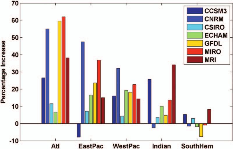
FIG. 5. Power dissipation index for each year from 1980 to 2006, from best-track data (blue) and simulations
(red), for each basin and for the global total. The correlation coefficient between the best-track and simulated
series is indicated in the upper-left corner of each panel, and the straight lines indicate the regression slopes of
each series. Power dissipation units are 1011 m3s –2 for the Atlantic, eastern North Pacific, and Southern Hemi-
sphere, 1010 m3s –2 for the north Indian Ocean, and 1012 m3s –2 for the western North Pacific and global total.

       The choice of the particular periods of time over    Calibration. The random seeding technique for gen-
    which to accumulate climate model statistics to drive   esis does not produce an absolute rate of genesis per
    our downscaling method was motivated almost             unit time per unit area. To calibrate the technique,
    entirely by the availability of daily model output      we set the global number of genesis events per year
    needed to derive the wind covariances. Given the        in each model to its observed global value in the
    noticeable multidecadal variability of some coupled     period of 1981–2000 for each of the twentieth-century
    climate models, even when driven with constant          simulations. The calibration constants thus derived
    climate forcing (Delworth and Mann 2000), 20 yr is      were then used for the A1b simulations. Thus, the
    probably insufficient for averaging over such natural   annual, global twentieth-century genesis rates are set
    variations in the climate simulations, and so the       to observations, but the rates are free to vary spatially
    comparison between the periods of 1981–2000 and         and seasonally, and to adjust to the different climate
    2181–2200 in any given model may be strongly            state of IPCC’s A1b scenario.
    affected if such variability is present. On the other      Because different models have different con-
    hand, the particular time scales of multidecadal        vection schemes with different thermodynamic
    variability vary substantially from model to model      constants and assumptions, each produces slightly
    (Delworth and Mann 2000), and so the ensemble of        different temperature profiles in convecting regions,
    model results may nevertheless be representative of     resulting in sometimes substantial differences in
    long-term climate change.                               potential intensity, calculated using the algorithm

356 |      MARCH 2008
TABLE 1. Models used—origins, resolution, designation, and calibration.
Potential intensity
Atmospheric Designation in
Model Institution multiplicative
resolution this paper
factor
Community Climate National Center for Atmospheric
T85, 26 levels CCSM3 1.2
System Model, 3.0 Research
Centre National de Recherches
CNRM-CM3 T63, 45 levels CNRM 1.15
Météorologiques, Météo-France
Australian Commonwealth Scientific
CSIRO-Mk3.0 T63, 18 levels CSIRO 1.2
and Research Organization
ECHAM5 Max Planck Institution T63, 31 levels ECHAM 0.92
NOAA Geophysical Fluid Dynamics 2.5°×2.5° 24
GFDL-CM2.0 GFDL 1.04
Laboratory levels
MIROC3.2 CCSR/NIES/FRCGC, Japan T42, 20 levels MIROC 1.07
mri_cgcm2.3.2a Meteorological Research Institute Japan T42, 30 levels MRI 0.97
described in Bister and Emanuel (2002; the algorithm century climate to historical data. Departures of the
itself is available as a FORTRAN subroutine online at simulated from the observed climatology may reflect
ftp://texmex.mit.edu/pub/emanual/TCMAX/). This imperfections of the technique itself, the model-
can result in quite different cumulative frequency simulated large-scale climates, or the climatological
distributions of storm lifetime peak intensity among tropical cyclone data. For the latter, we used best-track
the various models when simulating the climate of data from the period of 1981–2006 inclusive; these
the twentieth century. To correct for these model- data were obtained from the National Oceanic and
to-model differences, we adjusted the potential Atmospheric Administration’s National Hurricane
intensities of each model by a single multiplicative Center for the Atlantic and eastern North Pacific
constant in such a way as to minimize the differ- (Jarvinen et al. 1984; Landsea et al. 2004), and from
ences in the cumulative frequency distributions of the U.S. Navy’s Joint Typhoon Warning Center for the
storm lifetime peak wind speeds. These multiplica- rest of the world. Note that we did not seed the South
tive factors are listed in Table 1. Note that in this Atlantic in any of the simulations reported on here,
case, a single factor is applied to each model for all owing to the very large amount of computational time
ocean basins. Because potential intensity affects the required to produce a relatively low yield.
frequency of storms in our genesis technique, the Figure 6 compares the spatial distribution of gen-
calibration of potential intensity was done before esis points, integrated over the entire 20-yr period.
the frequency calibration. For both the best-track and synthetic data, genesis
In summary, a frequency calibration factor is defined as the first point in the record where the
was applied to each model’s global annual genesis peak 1-min wind at 10-m altitude equaled or exceeded
frequency, and each model’s global potential inten- 15 m s–1. The upper-left panel pertains to best-track
sity was likewise multiplied by a single factor. This data, while the remaining seven panels show results
guaranties that each model will produce roughly from each of the global models. Although the grossest
the correct cumulative frequency distribution of features of the observed distribution are well simu-
tropical cyclone lifetime peak wind speed in their lated by all the models, there are noticeable differ-
simulations of the last 20 yr of the twentieth century. ences among the models. In general, the observed
These calibrations are then held fixed in simulations distribution is more concentrated in the eastern
of different climates. North Pacific, and except for the Centre National de
Recherches Météorologiques (CNRM) and Model
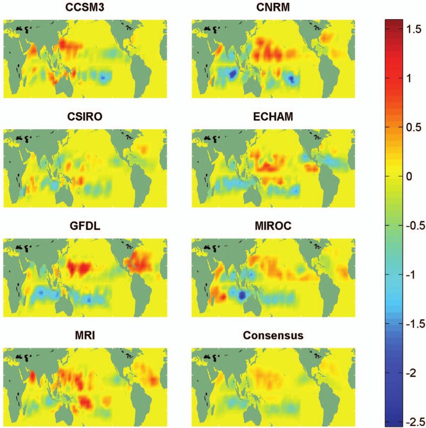
Quality of twentieth-century simulations. The quality for Interdisciplinary Research on Climate (MIROC)
of the simulated storms can be assessed against models, there is too much activity in the central
historical tropical cyclone data using a variety of North Pacific. Aside from these fairly systematic
metrics. Here we choose to compare the spatial and errors, each model has its own strengths and weak-
seasonal variability on the synthetic storms driven nesses in simulating the late-twentieth-century gen-
from simulations of the last 20 yr of the twentieth- esis distribution. For example, the third Community
AMERICAN METEOROLOGICAL SOCIETY MARCH 2008 | 357in the Atlantic, the models
produce too many storms
in winter and not enough
in summer. Likewise, in
the northern Indian Ocean,
the models produce too
many storms during the
midsummer lull in activity,
when there are very few
storms in nature. Here,
however, the observed dis-
tribution is calculated from
only a small number of
events in the 1981–2000
period, so care must be
exercised in assessing the
statistical significance of
the comparison.
A general impression
from these results is that
the models underestimate
the sensitivity of tropical
genesis rates in climate
variability, at least as mea-
sured by seasonal and spa-
tial variability. The distri-
butions in both space and
time are not as sharply
peaked as the distributions
calculated from histori-
cal tropical cyclone data.
Again, this may be because
the models may underpre-
dict the spatial and sea-
FIG. 6. Annual genesis distributions during the period of 1981–2006 for best- sonal variability of the re-
track data (upper-left) and for each of the seven models considered in this solved climate, or because
study. Shown is the logarithm of 1 + the genesis density accumulated over a of defects in the genesis-
5° × 5° grid; the color scale is the same in each case and identical to that used by-natural-selection tech-
in Figs. 1a,b. The model genesis distributions are based on 2,000 synthetic nique. Nevertheless, the
storms in each of the Atlantic, eastern North Pacific, western North Pacific,
gross features of the ob-
northern Indian, and Southern Hemisphere regions, while the best-track
data for this period include 303, 439, 773, 129, and 716 events in the respec- served spatial and seasonal
tive regions. variability of genesis rates
are sufficiently well simu-
Climate System Model (CCSM3) has practically no lated to make an examination of the sensitivity of
activity in the North Atlantic. simulated tropical cyclone activity to global climate
Figure 7 compares the annual cycle of genesis in worthwhile.
each of the seven models to historical data in each To assess the possibility that 20 yr is insufficient
of the five basins considered here. Again, the gross for averaging out natural multidecadal variability
features of the seasonal variability are captured by in the models, we obtained data from the period
most of the models, but there are interesting system- 1961–80 for the GFDL model to compare to the
atic errors. In the eastern North Pacific, there are simulations driven using data from 1981 to 2000.
too few synthetic storms in June and July, and far Simulated tropical cyclone activity was substantially
too many in October–December. In general, except less in the earlier period, with frequency as little
358 | MARCH 2008FIG. 7. Annual cycle of tropical cyclone counts during the period of 1981–2000, for each of the five main tropi-
cal cyclone regions (from top to bottom). The colored bars represent (from left to right) best-track data and
synthetic storms driven by output from the CCSM3, CNRM, CSIRO, ECHAM, GFDL, MIROC, and MRI models.
The annual total for each model is constrained to equal the observed annual total in each basin; the observed
basin counts are given in the caption to Fig. 6.
as half as great in some regions. This suggests that intensity achieved by the storms, their duration, and
comparisons between 20-yr periods in the twentieth their spatial distributions. In the following, we com-
and twenty-second centuries for at least some models pare certain key statistics of simulated activity in the
may be seriously affected by multidecadal variability, last 20 yr of the twenty-second century, compared to
a point we shall return to presently. Note that while the last 20 yr of the twentieth century.
the full range of radiative forcing variability owing Figure 8a shows the change in overall tropical
to greenhouse gases, aerosols, and volcanoes was cyclone power dissipation index by model and
included in the simulation, the natural, multidecadal basin. The power dissipation index was defined by
variability of the model would not necessarily have Emanuel (2005a) as the integral over the lifetime of
had the correct phase relationship with any such each storm of the maximum surface winds speed
variability in nature. cubed; this is a measure of the total amount of
kinetic energy dissipated by surface friction over
Comparison of late-twentieth-century to late-twenty- the lifetime of the storm. Here we accumulate the
second-century-tropical cyclone activity. Climate power dissipation over each basin and over the
change affects simulated tropical cyclone activity 20-yr period in question. The change is expressed
by changing the space–time probability of genesis, as 100 times the logarithm of the ratio of the power
the tracks taken by the simulated storms, and their dissipation values in the two simulations; for small
intensity evolution. These, in turn, affect the peak differences, this is approximately the percentage
AMERICAN METEOROLOGICAL SOCIETY MARCH 2008 | 359FIG. 8. Change in basinwide tropical cyclone (a) power dissipation, (b) frequency, (c) intensity, and (d) dura-
tion from the last 20 yr of the twentieth century to the last 20 yr of the twenty-second century, as predicted
by running 2,000 synthetic events in each basin in each period of 20 yr. The different colors correspond to the
different global climate models, as given in the legends. See text for definitions of intensity and duration. The
change here is given as 100 multiplied by the logarithm of the ratio of twenty-second- and twentieth-century
quantities. Note that (a) is the sum of (b)–(d). The values of the changes averaged across all models are given
by the numbers in black.
change. In general, there are substantial increases Pacific are indeterminate, but six out of seven models
in power dissipation in the western North Pacific show increases in the western North Pacific and
and decreases in the Indian Ocean and through the five out of seven models show increasing frequency
Southern Hemisphere, while the tendency is some- in the North Atlantic. Overall, the tendency of
what indeterminate in the eastern North Pacific, storm frequency is somewhat indeterminate in the
with large variability from one model to the next. Northern Hemisphere, but declines in the Southern
Four out of the seven models show appreciable in- Hemisphere.
creases in the North Atlantic, with the remaining Changes in the mean duration and intensity
three showing no change or decreases. of events are shown in Figs. 8c,d. Here we follow
Figure 8b shows the percentage change in the Emanual (2007) in defining duration as
frequency of all events that achieve a peak wind
speed of at least 21 m s –1. There is a general ten-
(1)
dency toward decreasing frequency of events in the
Southern Hemisphere, but the percentage change
in frequency is not usually as large as the decrease where N is the sample size, Vimax is the maximum
in power dissipation, showing that the latter is also wind of storm i at any given time, Vismax is the lifetime
affected by decreasing intensity and/or duration. maximum wind of storm i, and τi is the lifetime of
Changes in overall frequency in the eastern North each storm. This velocity-weighted duration assigns
360 | MARCH 2008relatively little weight to long periods at which storms frequency in the Bay of Bengal and in the eastern and
sometimes exist at low intensity. The mean intensity far western portion of the North Pacific, while there
is defined as is some indication of increasing activity in the main
development region of the western North Pacific. The
model consensus has slightly decreased frequency of
(2) events in the Caribbean and in the western portion of
the Atlantic main development region, with a notice-
This is the mean cube of the maximum wind speed ably increased frequency in the far eastern portion of
accumulated over the lifetime of each storm, divided the tropical Atlantic and in the subtropics, including
by the duration as defined by (1). Note that the off the southeast U.S. coast.
power dissipation is just the product of the overall These results suggest potentially substantial
frequency, duration, and intensity as defined above; changes in destructiveness of tropical cyclones as a
thus, the logarithms of these quantities are additive consequence of global warming. But large model-to-
and Figs. 8b–d add up to Fig. 8a. Figure 8d shows little model variability and natural multidecadal variabil-
change in the velocity-weighted duration of events, ity within at least some of the models also suggests
but with a tendency toward decreasing duration in the large uncertainty in such projections, reflecting the
Southern Hemisphere and north Indian Ocean, and uncertainties of climate model projections in general
slight increases elsewhere. As expected from theory and the influence of natural variability. Ideally, we
and previous numerical simulations, there is an over- would like to compare simulations driven by climate
all tendency toward increased intensity of storms, but model data accumulated over periods long enough
some models show decreases in some basins. both to quantify and account for the effects of natural
We also calculated basin-averaged changes in variability, but because such data are not currently
sea surface temperature and potential intensity, available, this is left to future work.
defining the averaging areas to coincide roughly with
conventional definitions of tropical cyclone main DISCUSSION. The findings presented here are
development regions. Curiously, there is no system- largely consistent with those obtained by direct
atic correlation between changes in any of the metrics simulation of tropical cyclones by global models
described in this section with changes in either sea as well as by downscaling using regional models
surface temperature or potential intensity averaged embedded in global models. The majority of such
over the individual basins. This contrasts sharply exercises to date show a decrease in global genesis
with the high correlation between variations in rates, as summarized, for example, by Bengtsson
observed Atlantic tropical cyclone power dissipation et al. (2007). For example, recent global model-based
and sea surface temperature, reported by Emanuel studies (e.g., Bengsson et al. 1996; Sugi et al. 2002;
(2005a), and the relatively high correlation among Oouchi et al. 2006; Yoshimura et al. 2006; Bengtsson
year-to-year variability of power dissipation, sea et al. 2007) all show decreasing frequency of tropi-
surface temperature, and potential intensity in the cal cyclones globally, although some studies show
simulations forced by reanalysis data in the years regional increases. This is encouraging, because the
of 1980–2006. Deconvolving the various environ- route to genesis in the method described here is quite
mental factors responsible for the changes in the different from that operating in climate models;
various tropical cyclone metrics described here is one potentially serious limitation of our technique
the subject of ongoing work and will be reported in is the assumed constant amplitude and frequency
the near future. of potential initiating disturbances. Because tropi-
Changes in the spatial patterns of genesis are cal cyclones evidently arise from finite-amplitude
shown in Fig. 9 for each of the seven models and the instability (Emanuel 1989), the prevalence and
average over all models. While there is much variation characteristics of potential initiating disturbances
from one model to the next, several patterns emerge should be important, and these can be expected to
in the consensus that seem common to most models. depend on the climate state. At the same time, this
As noted before, most models show declining fre- limitation might be expected also to affect the qual-
quency throughout the Southern Hemisphere, except ity of the seasonal cycle of tropical cyclone activity,
for small regions east of Indonesia and the far western yet the technique does reasonably well with this
south Indian Ocean. Many individual models, as well (see Fig. 3).
as the model consensus, show increased frequency in Some of the biases evident in the distributions
the northern and western Arabian Sea, but decreased of genesis events (see Fig. 6) are also common to
AMERICAN METEOROLOGICAL SOCIETY MARCH 2008 | 361FIG. 9. Change in genesis density from the last 20 yr of the twentieth century to the last 20 yr of the
twenty-second century, as predicted by running 2,000 synthetic events in each basin in each period of
20 yr for each model and for the average (“consensus”) over all models. The color scale is the same
for all figures and is in units of number of events per 5° lat–lon square yr–1.
explicitly produced events in climate models. For differ, however; whereas the present study compares
example, it is common to produce too many events the last 20 yr of the twentieth and twenty-second
in the central North Pacific, and the geographic centuries, the Bengtsson et al. study compares the
distributions are generally broader than observed last 30 yr of the twentieth and twenty-first centuries.
(Camargo et al. 2005). This suggests that some of the Because in scenario A1b, CO2 does not level off until
defects in the genesis distributions noted here can be the year 2100, some additional warming will have
attributed to biases in the large-scale environment, occurred by the end of the twenty-second century.
though others no doubt arise from the assumption of The output used to drive the synthetic tracks shown
uniform or vorticity-weighted seeding amplitude. here was taken from the T63 version of ECHAM5;
Of particular interest is the recent work by Bengtsson et al. also report T63 results, but examined
Bengtsson et al. (2007), who used one of the models higher-resolution output as well. Curiously, the gen-
(ECHAM5) included in this study; thus a direct esis distributions produced directly by ECHAM5 also
comparison can be made. The time periods examined show too many events in the central North Pacific
362 | MARCH 2008(see their Fig. 6a), as does the present technique The quantity χm measures the relative importance
(Fig. 6 herein). Both techniques predict decreases in of downdrafts and surface fluxes in controlling the
the frequency of events in all basins, except that our entropy of the subcloud layer. It is an important
technique predicts a modest increase in the western parameter in the formulation of the boundary layer
North Pacific. As in the present study (Fig. 8c), the quasi-equilibrium closure for convective updraft
intensity distributions shown by Bengtsson et al. mass fluxes used in the CHIPS model and elsewhere
exhibit a tendency for increased frequency of the (Emanuel 1995). For example, in CHIPS, the convec-
higher-intensity events, and this becomes more pro- tive updraft mass flux is given by
nounced at higher spatial resolution. Note, however,
that in these and the other direct GCM simulations, (5)
the intensity distributions of explicitly modeled
storms are truncated at the high end compared to na- where w is the large-scale vertical velocity at the top
ture, probably because of the relatively low horizontal of the boundary layer, Ck is the surface exchange
resolution of the model. coefficient for enthalpy, and |V| is the surface wind
Thus, the present results are broadly consistent speed. Thus, χm also determines the rates of increase
with those of global model studies in that both gen- of convective updraft with surface wind.
erally show an increased frequency of very intense The CHIPS model has only one layer in the middle
storms, but some tendency toward a reduction in troposphere, in which χm is defined. When it is run
the overall frequency of events in the Southern in forecast mode, or used in the synthetic track
Hemisphere. The simplicity of the intensity model technique, sm is defined at 600 hPa, which is usually
and natural selection technique employed here allows close to the level at which it attains a minimum value
us to draw a fairly definitive conclusion about why in the tropics.
the frequency of events declines in some places in In regions susceptible to tropical cyclones, the
our simulations. atmosphere is approximately neutral to moist convec-
An important nondimensional parameter in the tion and the lapse rate of the troposphere is nearly
CHIPS intensity model is the normalized difference moist adiabatic. Thus,
between the moist entropy of the middle troposphere
and that of the boundary layer. This parameter, called (6)
χ m in the various papers that describe the model
(Emanuel 1989, 1995), was shown to be important where s * is the (approximately constant with height)
in regulating how long it takes an initial disturbance saturation entropy of the troposphere above the
to moisten the middle troposphere to the point that boundary layer. Thus, it should not matter at which
intensification can occur; the larger it is, the longer level we choose to calculate it, so we again choose
the gestation period. 600 hPa. Using the definition of moist entropy (see,
The specific definition of χm is e.g., Emanuel 1994), the numerator in (3) can then
be approximated as
(3)
(7)
where sm, sb, and s0* are the entropies of the middle where q* is the saturation specific humidity and the
troposphere and boundary layer, and the saturation quantities are evaluated at 600 hPa.
entropy of the sea surface, respectively. The moist The quantity q* does not vary much in the tropics,
entropy is defined (Emanuel 1994) as either in space or with time, because of the strong
dynamical constraint on the magnitude of the tem-
(4) perature gradient, owing to the small value of the
Coriolis parameter. Thus, in the present climate,
where for simplicity we have neglected the depen- seasonal and spatial variations in sb – sm as given by (7)
dence of the heat capacities and gas constants on the are dominated by variations in relative humidity. But,
water content. Here cp is the heat capacity at constant under global warming, changes in χm at fixed points in
pressure of air, Lv is the latent heat of vaporization, space are dominated by changes in q*, while the rela-
q is the specific humidity, Rd is the gas constant for tive humidity stays approximately constant (at least in
dry air, Rv is the gas constant for water vapor, and H most climate models). In fact, globally, we can predict
is the relative humidity. that the magnitude of χm should generally increase
AMERICAN METEOROLOGICAL SOCIETY MARCH 2008 | 363You can also read