Hydraulic characterization and upscaling of fracture networks based on multiple-scale well test data
←
→
Page content transcription
If your browser does not render page correctly, please read the page content below
WATER RESOURCES RESEARCH, VOL. 36, NO. 12, PAGES 3481–3497, DECEMBER 2000

Hydraulic characterization and upscaling of fracture
networks based on multiple-scale well test data
Auli Niemi,1 Kimmo Kontio, and Auli Kuusela-Lahtinen
Communities and Infrastructure, Technical Research Centre of Finland, Espoo, Finland

Antti Poteri
Energy, Technical Research Centre of Finland, Espoo, Finland

Abstract. Hydraulic properties and upscaling characteristics of low-permeability fractured
rock are analyzed based on systematic well test data from three different measurement
scales. First, tests are simulated in a large number of geological fracture network
realizations, and the acceptable fracture transmissivity distribution parameters that
produce the observed statistics of the two smallest measurement scales, i.e., 2-m and 10-m
scales, are defined. Instead of a single value, a range of acceptable parameter values can
be found to produce the observed result. Second, upscaling simulations are carried out
with the calibrated networks. These indicate that the investigated system cannot be
properly modeled by means of a continuum tensor presentation but would better be
represented by means of “equivalent fracture” statistics. Third, the conductive
characteristics of the calibrated 30-m network blocks are compared to well test results
from the same scale. The results from this preliminary analysis indicate that one-
dimensional borehole observations interpreted with standard continuum-based methods
may considerably underestimate the three-dimensional conductive characteristics of
heterogeneous, noncontinuum fractured media.

1.   Introduction                                                      falls between these two, that is, scales too large for fracture
                                                                       network models but small enough so that heterogeneity of rock
   During the last 15 to 20 years, great progress has been made        outside the major deterministic fracture zones is still of inter-
in developing tools and gaining an understanding of the gen-           est. The range of applicability of each approach, especially the
eral behavior of the hydrology of fractured rocks, both at the         transition from fracture network– based approaches to contin-
level of individual fractures [Moreno et al., 1990; Cvetkovic,         uum-based approaches, also depends on the characteristics of
1991; Tsang et al., 1991; Tsang and Neretnieks, 1998; Painter et       the rock in question. Continuum behavior is more likely to
al., 1998; Cvetkovic et al., 1999] and at the level of field-scale     occur in densely fractured, well-connected fracture networks
fracture systems [e.g., Neuman and Depner, 1988; Neuman,               with mixed fracture orientations than in sparsely fractured,
1987; Cacas et al., 1990; Dershowitz et al., 1991; Herbert et al.,     poorly connected, and/or strongly anisotropic systems [e.g.,
1991; Long et al., 1992; Gavrilenko and Gueguen, 1998]. The            Long et al., 1982].
modeling approaches for field-scale fractured media can be
                                                                          The support scale and the related conductivity statistics of
divided into three basic categories: (1) deterministic porous
                                                                       stochastic continuum models can be determined either directly
medium approaches, (2) fracture network approaches, and (3)
                                                                       from hydraulic well test data or by means of fracture network
stochastic continuum approaches. As the relative significance
                                                                       modeling. In the first approach, originally proposed by Neu-
of local heterogeneities decreases with increasing scale, the
                                                                       man [1987] and subsequently applied by several others [e.g.,
range of applicability of these approaches depends on the scale
                                                                       Neuman and Depner, 1988; Follin and Thunvik, 1994; Tsang et
of interest. Because of computational constraints, fracture net-
                                                                       al., 1996], the variability in borehole hydraulic conductivity
work models can usually be applied for a scale of at most a few
                                                                       data is introduced directly into Monte Carlo type simulation
hundreds of meters. In deterministic porous medium ap-
                                                                       models by using the scale of field measurements as the scale of
proaches the medium properties are assumed fixed and known;
                                                                       the model permeability zones. While this is attractive in its
major fracture zones are imbedded deterministically, and the
                                                                       practicality, the critical question is whether the medium prop-
remaining part of the rock is assigned averaged properties.
These approaches are applicable in the largest of scales when,         erties are such that an equivalent continuum presentation is
for example, the effect of major fracture zones is investigated        justified at the scale of the measurement. In other words, can
and the effect of local heterogeneities is not of interest. The        one with reasonable accuracy present the hydraulic conductiv-
range of applicability of the stochastic continuum approaches          ity structure of the rock with an equivalent continuum conduc-
                                                                       tivity tensor. The second approach, in which the continuum
                                                                       properties are calculated by means of fracture network mod-
  1
    Now at Department of Earth Sciences, University of Uppsala, Upp-   eling, also allows the applicability of this assumption to be
sala, Sweden.
                                                                       studied. This approach has been applied, for example, for
Copyright 2000 by the American Geophysical Union.                      Stripa data in Sweden by Herbert et al. [1991] and by Dershowitz
Paper number 2000WR900205.                                             et al. [1991] and for Fanay-Augeres data in France by Cacas et
0043-1397/00/2000WR900205$09.00                                        al. [1990]. La Pointe et al. [1995] looked at the continuum

                                                                   3481
3482 NIEMI ET AL.: HYDRAULIC CHARACTERIZATION OF FRACTURE NETWORKS
conductivity characteristics for the Äspö site in Sweden. Using to 1000 m. The distances between the boreholes are of the
fracture network modeling for determining the continuum order of a few hundreds of meters.
conductivities has the benefit of being able to take heteroge- Hydraulic single-hole tests have been carried out with a fixed
neity into account more realistically, starting from the geolog- interval length in these boreholes; the total length of the bore-
ical characteristics. Conversely, a large number of parameters holes tested was over 5000 m. Two different testing methods
have to be calibrated, and immense amounts of data are and three different measurement scales have been used. The
needed for this calibration. constant pressure injection method has been applied with
Most of the aforementioned studies have been related to 30-m, 10-m, and 2-m packer spacings, and the so-called differ-
small-scale field studies in field laboratory settings. They have ence flow method has been applied with 2-m and 10-m packer
employed short distances between the boreholes, so that cross- spacings. While the constant pressure injection method is
hole and tracer information has been available to validate the widely used for testing low-permeability media and described
results. Furthermore, they have often concentrated on the up- in a number of references [e.g., National Research Council,
per hundreds of meters of the bedrock with relatively high 1996], the latter method is less common and deserves a brief
transmissivities and well-connected fracture networks. Reflect- description. In the method, for each isolated test section in
ing this, the continuum scales employed have been of the order turn, the steady state flow rate into or out of the borehole is
of 10 m or below. An exception was the study by La Pointe et measured corresponding to two different prevailing borehole
al. [1995] where support scales of the order of 50 m were also pressures. Assuming a radial flow field, hydraulic conductivity
used. This study also considered greater depths with data up to is determined based on the two pressure–flow rate data pairs
600 to 800 m. Especially in the case of site characterization for obtained this way. The method has been thoroughly tested and
nuclear waste disposal, one is interested in the flow on large widely used especially in the Finnish waste isolation program
scales and at great depths. In such settings, fracture networks as well as in some international waste isolation experiments
are less connected and of lower conductivity than in the upper [Rouhiainen, 1998; Rouhiainen and Heikkinen, 1998, 1999].
parts of the rock. Interference tests and model calibration do More detailed description of the method is given by Hinkkanen
not capture the small-scale heterogeneity observed in bore- et al. [1996].
holes but rather are dominated by large-scale features. To The rationale of the testing program was that sections found
carry out interference tests that would characterize the average intact with larger test intervals were not retested with the
“nonzone” rock, i.e., the rock outside the deterministic frac- smaller interval. All boreholes were systematically scanned ei-
ture zones, one would need very long times or, alternatively, ther with 30-m or with 10-m packer spacing, and some bore-
short distances between the boreholes. These, in turn, would holes were scanned with both. After this, 2-m tests were done
only cover a small part of the investigated rock. in sections found conductive with the larger test intervals. The
The major questions to be addressed then are how to deter- 2-m-scale difference flow measurements were done systemat-
mine the hydraulic properties of the fracture networks in the ically in all conductive sections. Testing with the 2-m-scale
“nonzone” average rock, how much data are needed for this, constant head injection method was not quite as systematic but
and what the resulting uncertainty is in the network properties. done more to get a comparison database for the 2-m difference
We will address these questions by using field data from the flow data. An example of a borehole hydraulic conductivity
Romuvaara crystalline rock site in Kuhmo, Finland, as the profile as obtained with different measurement methods and
example database. More specifically, we will look at (1) the scales is shown in Figure 1. The data on fracture geometry
possibility of using single-hole hydraulic data from different come from mappings of surface outcrops and investigation
measurement scales to estimate the hydraulic properties of dikes as well as geological mappings of core samples that were
fracture networks and (2) how much uncertainty and non- available for all boreholes. The fracture size distribution was
uniqueness there is in such estimates. Second, we will look at determined from surface observations and the position data
the upscaling properties of the networks. More exactly, we will from core samples and, to some extent, also from borehole
(3) estimate the continuum versus discontinuum behavior of TV-camera observations. The fracture observations have been
the upscaled networks and, (4) if applicable, determine the interpreted by applying an assumption of statistical homoge-
continuum conductivity tensor distributions that can be used, neity of the fracturing geometry in the investigated volume of
for example, as inputs for large-scale Monte Carlo simulations. rock. It should be pointed out that surface fractures have been
Finally, we will (5) compare the network-based “upscaled” subject to erosion, and it is not clear that they are representa-
conductivities to those directly determined from well tests of tive of the fractures at depth, but these differences cannot be
the same scale by means of traditional well test analyses. quantified without excavated underground tunnels. Because of
the biased nearly vertical orientation of the boreholes, the
fracture orientation data were corrected as described by Poteri
2. Data Characteristics and Laitinen [1997].
2.1. Site Description and Data Collection In the present study, the main interest is in the characteris-
The example data come from the Romuvaara site. This tics of the rock outside the deterministic fracture zones. There-
crystalline rock site is located in eastern Finland and has been fore data sections related to fracture zones were excluded from
investigated as a potential candidate for the disposal of high- the hydraulic and fracture geometry databases before the sta-
level nuclear waste. The data analyzed here do not attempt to tistical analyses. The question of what conductive feature is
reflect all the characteristics of Romuvaara in a site character- deterministic and what is stochastic is not well defined in hy-
ization sense but should rather be considered as representative drology of fractured rocks, and some subjectivity usually re-
of a low-conductivity fractured rock. The site is characterized mains in the interpretation. In the present work a conservative
by relatively low overall conductivity, with a decreasing trend in interpretation was used in terms of the average rock, and
conductivity with depth. The data come from altogether nine features that were “uncertain” were assigned to the stochastic
subvertical deep boreholes, ranging in depth from about 300 m rather than deterministic data pool [Niemi et al., 1999].NIEMI ET AL.: HYDRAULIC CHARACTERIZATION OF FRACTURE NETWORKS 3483
Figure 1. Example hydraulic conductivity profiles obtained with different methods and measurement scales;
difference flow measurements with (a) 2-m and (b) 10-m packer spacing and constant head injection mea-
surements with (c) 30-m, (d) 10-m, and (e) 2-m packer spacing from Romuvaara borehole KR3.
2.2. Fracture Geometrical Properties and size distribution have been estimated independently using
According to the approach presented in more detail by Po- borehole and outcrop data for the fracture orientations and
teri and Laitinen [1997], the statistical properties of the geo- sizes, respectively. Parameters of the orientation and size dis-
metrical fracture data have been determined for fracture ori- tributions have been calculated by minimizing the squared
entation, size, and fracture intensity. No correlation is assumed difference between the measured and simulated distributions.
to exist between the fracture orientation and size. Orientation The spatial model of the fracturing assumes that the centers of
the fractures are uniformly distributed in the modeling volume.
On the basis of this assumption the fracture intensity is calcu-
Table 1. Parameters of the Fitted Probability Functions of lated from the mean fracture frequency along the boreholes.
Fracture Geometrical Properties With Borehole Depths Only fractures classified as open or filled, and thus potentially
⬎200 m water-conducting, were included in the analysis. As an analysis
tool, the Fracman fracture network generation program by
Parameter Value Open Filled
Dershowitz et al. [1996a] was used. The algorithm allows com-
Fracture orientation parameters a plex fracture geometries to be generated based on fracture
Mean orientation trend 37.0 47.1 geometric data, and it has been extensively tested and verified
Mean orientation plunge 59.0 41.2 for this type of analyses [Dershowitz et al., 1996b].
Dispersion coefficient K 2.35 2.24
Intensity P 32 0.75 1.48 The fracture orientations are described by means of a Fisher
Size distributionb distribution, with parameters for mean pole trend and plunge
Mean 0.65 1.5 (, ) and dispersion as given in Table 1. The expression for
Standard deviation 0.7 0.45 the appropriate Fisher distribution for directional data is
a
This is a Fisher distribution. (e.g., from Mardia [1972], as applied by Chiles and de Marsily
b
This is a lognormal distribution. [1993])3484 NIEMI ET AL.: HYDRAULIC CHARACTERIZATION OF FRACTURE NETWORKS
This is an isotropic unimodal distribution, where ⬘ and ⬘ are
independent random variables and is the Fisher distribution
parameter. Distribution is rotational symmetric around the
mean orientation. This is reflected in (1) that is not dependent
on the phase angle ⬘ which is an independent uniform ran-
dom variable in the range of [0, 2]. The fractures were as-
sumed to be circular, with the radius being lognormally dis-
tributed. It was assumed that the fractures do not terminate at
the intersections with other fractures. Fracture intensity is de-
scribed through P 32 [L ⫺1 ] [Dershowitz et al., 1996a]
P 32 ⫽ A f/V t, (2)
where A f is the total area of the fractures and V t is the total
volume of the model. In Table 1, only data below 200-m depth
are shown. The division into depth intervals of above and
below 200 m by Poteri and Laitinen [1997] is based on earlier
studies showing a statistical difference in the hydrological data
between the upper and lower parts of the rock [e.g., Niemi and
Kontio, 1993]. In generating the fractures, the enhanced Bae-
cher model [Baecher et al., 1977] was used. The fracture centers
are located uniformly in space, following a Poisson process.
The enhanced Baecher model allows provisions for fracture
terminations and general fracture shapes [Derschowitz et al.,
1996a]. The uncertainties related to geometrical fracture sta-
tistics were not investigated here, but these properties are
assumed fixed. Emphasis is placed on studying the hydrological
data.
2.3. Hydrological Data
For determining the hydraulic properties of the fracture
networks, the fixed-interval length hydraulic well test data from
different scales is used. The rationale for utilizing these data
was as follows: (1) The data from the finest scale (2-m data) are
used for obtaining an initial estimate for individual fracture
transmissivities. (2) The data from the 10-m scale are used as
the basis for the hydraulic fracture network calibration. Exten-
sive numerical simulations are carried out with fracture net-
work models to obtain the best estimate for fracture transmis-
sivity distributions that would yield the observed 10-m well test
results. (3) The 30-m scale constant head injection test data are
used as comparison material for the conductivities determined
with network simulations of the same scale.
Histograms of the log transmissivities for the 2-m and 10-m
data at the two depth intervals are given in Figures 2a–2d.
From Figure 2 it can be observed that the portion of the
nonconductive sections is significant in all of the data sets,
being larger with the small test interval and in the deeper part
of the bedrock. The higher number of nonconductive sections
in deeper parts of the rock is due to an actual decrease of
conductivity with depth. This is a well-known phenomena in
this type of fractured crystalline rock where the increase in
lithostatic pressure tends to close the fractures. The higher
Figure 2. Histograms of transmissivity data obtained (a) with number of nonconductive sections with the smaller test inter-
2-m difference flow measurements for borehole depths ⬍200 val, however, is due to the fact that the higher testing interval
m (n ⫽ 375) and (b) borehole depths ⬎200 m (n ⫽ 275) as “averages out” heterogeneity. Only one fracture can create a
well as (c) for data obtained with 10-m constant head injection “nonzero” hydraulic conductivity value in the 10-m-scale data,
measurements for borehole depths ⬍200 m (n ⫽ 66) and (d)
while the same fracture would create one “nonzero” and four
borehole depths ⬎200 m (n ⫽ 51).
“zero” conductivity values in the 2-m-scale data.
2.4. Initial Estimates for Fracture Transmissivity
1 sin ⬘ and Storage Properties
f共 ⬘, ⬘兲 ⫽ exp 共 cos ⬘兲, (1)
2 共e ⫺ 1兲 The first estimate of fracture transmissivities is based on the
0 ⱕ ⬘ ⱕ / 2, 0 ⱕ ⬘ ⱕ 2. observed fracture densities and hydraulic conductivity mea-NIEMI ET AL.: HYDRAULIC CHARACTERIZATION OF FRACTURE NETWORKS 3485
surements at the 2-m scale. On the basis of the approach Table 2. Statistics of Measured and Best Fitting Modeled
developed by Osnes et al. [1988] and implemented by Dershow- 2-m Scale Fixed Interval Length (FIL) Data Along With
itz et al. [1996a], we assume that the transmissivity of each test Fracture Transmissivity Data Yielding the Fita
interval is equal to the sum of the conductive fracture trans-
missivities in that interval. In other words, the fractures are 2-m FIL Data Parameter Simulated Measured
assumed to be independent of each other: Mean 3.5 ⫻ 10 ⫺8
5.9 ⫻ 10⫺9
Standard deviation 3.5 ⫻ 10⫺7 3.2 ⫻ 10⫺8
冘
ni
Log10 mean ⫺10.2 ⫺10.2
Ti ⫽ T ij, (3) Log10 std deviation 0.99 1.0
j⫽1 Skewness 13.4 9.2
Nonconductive, % 69.1 75.6
where T i is the transmissivity of the ith packer interval, n i is
the number of conductive fractures in the interval, and T ij is Fracture Parameter Value
the transmissivity of the jth conductive fracture within the ith b
Best fitting fracture transmissivity m ⫽ ⫺13.4
interval. Within any given interval the number of conductive
⫽ 2.6
fractures n i is assumed to be a random number following a Fracture density 1.32 fractures m⫺1
Poisson distribution
a
Model assumes fractures are independent. Borehole depth is ⬎200 m.
n ne ⫺n b
Values are calculated as log10 of fracture transmissivities.
f n共n兲 ⫽ , (4)
n!
where n is the Poisson process rate and equal to the expected S ⫽ T, (5a)
value of n. The conductive fracture frequency is given by f c ⫽
n/L i , where L i is the length of the test zones. The distribution S ⫽ 0.001 冑T, (5b)
of fracture transmissivities T ij is described by a lognormal
S ⫽ C 冑3 T, (5c)
distribution, defined with a mean and standard deviation. In
the numerical implementation of Fracman used here [Der- where C is a constant depending on the physical properties of
showitz et al., 1996a], for a given set of the parameters describ- water and aperture characteristics of the fractures. The first
ing the transmissivity distribution f(T ij ) and conductive frac- relation is based on the observation that in several cases shown
ture frequency f c , the distribution of packer interval in Table 3, the diffusivity ⫽ T/S is of the order of 1, with
transmissivities f(T i ) is found by Monte Carlo simulation, and storativity with respect to either a mean transmissivity or a
the best fitting value is found by simulated annealing search fixed single-value transmissivity. The second relation is the
routine. The measured and the best fitting modeled density empirical relation by Uchida et al. [1994] based on field data
histograms for the 2-m interval test data are shown in Figure 3. from the Äspö Hard Rock Laboratory in Sweden. The third
The corresponding parameter values are summarized in relationship comes from the definition of storativity,
Table 2.
Transient fracture network simulations also require infor- S ⫽ gb共 ␣ ⫹  兲, (6a)
mation on fracture storativities (S). Such data do not exist for 3 ⫺3
where is the density of water [M L ], g is acceleration due
the average rock from the site. Therefore values reported in to gravity [L T ⫺2 ], and b is the characteristic aperture [L], in
the literature for similar sites were reviewed, and a summary is this case the aperture controlling the fracture storage proper-
given in Table 3 along with the corresponding ranges of frac- ties,  [L M ⫺1 T 2 ] is the compressibility of water, ␣ [L M ⫺1
ture transmissivities T [L 2 /T]. In the present study, three T 2 ] the compressibility of the medium, and is the fracture
relationships are tested for fracture storativities porosity. Assuming the medium is incompressible and setting
the porosity equal to 1, that is, assuming a fully open fracture,
we get
S ⫽ gb storage . (6b)
The aperture b storage is the volumetric aperture controlling the
storage properties and is usually larger than the hydraulic
aperture controlling transmissivity. The hydraulic aperture
(b hydr), in turn, can be determined from fracture transmissivity
T [m2 s⫺1] based on the well-known cubic law for laminar flow
in open parallel-wall fractures [Witherspoon et al., 1980]
3
g b hydr
T⫽ . (7)
12
Deriving hydraulic aperture from this expression, (5c) can be
derived from (6). A ratio b storage/b hydraulic ⫽ 10 was used here,
resulting in a value of C ⫽ 4.4 ⫻ 10 ⫺7 [(s m⫺2)1/3]. Obvi-
Figure 3. Cumulative frequencies of measured and best fit- ously, in natural fractures this ratio can have a wide range of
ting modeled 2-m fixed interval length (FIL) data with the values, depending on the variability of the aperture structure of
Osnes et al. [1988] model used to get the first estimate for the fracture in question. A comprehensive overview and dis-
fracture transmissivities. Fractures are assumed to be indepen- cussion concerning the meaning of different equivalent frac-
dent (d ⬎ 200 m). ture apertures and their interpretation from hydraulic and3486 NIEMI ET AL.: HYDRAULIC CHARACTERIZATION OF FRACTURE NETWORKS
Table 3. Fracture Storativity and Corresponding Transmissivity Data Used in Various Fracture Network Simulation Studies
Reference T (m, ) a S Site
⫺7 ⫺7 ⫺8
Derschowitz et al. [1991] 2 ⫻ 10 , 4 ⫻ 10 1 ⫻ 10 Stripa crown fractures
1 ⫻ 10⫺8, 5 ⫻ 10⫺6 1 ⫻ 10⫺8 Stripa nonzone
2 ⫻ 10⫺8, 4 ⫻ 10⫺7 1 ⫻ 10⫺8 Stripa fracture zone
1 ⫻ 10⫺7, 3 ⫻ 10⫺9 1 ⫻ 10⫺8 Stripa fracture zone
1 ⫻ 10⫺8, 1 ⫻ 10⫺9
2 ⫻ 10⫺8 䡠 䡠 䡠 3 ⫻ 10⫺5b 6 ⫻ 10⫺9 䡠 䡠 䡠 2 ⫻ 10⫺4 Stripa fracture zone
Long et al. [1992] 2 ⫻ 10⫺6 䡠 䡠 䡠 1 ⫻ 10⫺5c 1 ⫻ 10⫺5 Stripa fracture zone
Uchida et al. [1994] 4 ⫻ 10⫺7, 7 ⫻ 10⫺6 0.001T 0.5 Äspö nonzone
Winberg [1996] ⫺8.4, 0.9d 0.001T 0.5 Äspö nonzone
La Pointe et al. [1995] 9 ⫻ 10⫺7, 5 ⫻ 10⫺6 1 ⫻ 10⫺6 Äspö nonzone
a
This is a lognormal distribution.
b
A range of values is indicated.
c
A channel conductance is indicated; units are in m3 s⫺1.
d
Parameters m and are in log10 space.
tracer studies is given by Tsang [1992]. Hakami [1995] docu- each fracture is modeled according to the continuity equation
ments aperture data for a number different types of fractures for saturated groundwater flow in two dimensions
as measured in laboratory conditions.
⭸h
2.5. Autocorrelation in Hydraulic Conductivity T ⵜ 2h ⫽ S ⫹ q, (9)
⭸t
The autocorrelation structure of hydraulic conductivity can
where ⵜ2 is the Laplacian operator, h is hydraulic head [L], q
be estimated by means of variogram analysis of the well test
refers external sources and sinks [L T ⫺1 ], and t is time [T].
data. This is usually expressed in terms of a so-called semiva-
For modeling the flow in the three-dimensional networks of
riogram [e.g., Journel and Huijgbregts, 1978] for a general ran-
two-dimensional fractures, the MAFIC (Matrix Fracture In-
dom variable Z:
teraction Code) model [Miller et al., 1995] was used. The pro-
␥ 共h兲 ⫽ 21 E兵关Z共x ⫹ h兲 ⫺ Z共x兲兴 2其, (8) gram uses the Galerkin finite element approximation for the
numerical solution. It is interfaced with the Fracman fracture
where ␥ is the semivariogram, E is the expected value, x is the network generation program via a specific mesh generation
position vector, and h is the distance vector between two routine [Dershowitz et al., 1996a]. The models have been tested
points. Here the variograms were determined from the 2-m and verified against numerous test cases and applied to several
hydraulic conductivity data. Various subsets were considered field data studies (for summary see Dershowitz et al. [1996b]).
by Niemi et al. [1999], but only the main findings will be ad- For the present study, the mesh generation routines were
dressed here. Figure 4 shows what could be considered as the somewhat enhanced, and some additional test simulations
most representative variogram for the 2-m scale conductive were carried out by studying the performance of the algorithms
data in the average “nonzone” rock. In the underlying data all in well-defined cases where the results could be compared
the boreholes are combined into one data set, and only varia- against analytical solutions. This was done to investigate the
tion along the borehole length is observed. This was done in effect of various numerical factors on the simulated results so
order to make the data sets sufficiently large to produce rep-
resentative variograms. Data from both depth intervals (d ⬍
200 m and d ⬎ 200 m) is combined for the same reason. In
this type of crystalline rock, where the rock type remains the
same and the decrease in overall permeability with depth is
due to the continuous increase of lithostatic pressure, there is
actually no particular reason to expect the autocorrelation to
be especially sensitive to depth. So in this respect combining
the data can be seen to be reasonable. Furthermore, quite a
significant part of the data that are at the detection limit are
excluded, because including them yielded variograms that re-
flect the extent of the intact or “nonmeasurable” sections
rather than the correlation structure within the conductive
sections. The resulting variogram, determined with the model
of Englund and Sparks [1991], is given in Figure 4. It shows a
range of 8 to 10 m. The variogram sill captures about 85% of
the corresponding sample variance (2 ⫽ 1.17) which can be
considered a good agreement in the case of real field data.
3. Numerical Model for Fracture Network
Flow Simulations
In the analyses, transient groundwater flow in three- Figure 4. Variogram of the 2-m flow meter data when data
dimensional networks of fractures is considered. The flow in at detection limit is excluded.NIEMI ET AL.: HYDRAULIC CHARACTERIZATION OF FRACTURE NETWORKS 3487
that the most optimal computational options could be selected the borehole walls of that section, representing the constant
for the actual network simulations. These test simulations are head injection. As in the actual tests, an overpressure of h ⫽
presented in more detail by Niemi et al. [1999]. 20 m (expressing the pressure in terms of hydraulic head) is
In the test simulations a constant-head injection test in an used in the borehole for the duration of 15 min. The injection
isolated horizontal fracture intersecting the borehole was con- flow rate required to maintain this overpressure is observed.
sidered. The simulated result was compared to the correspond- The upper and lower boundaries, as well as the outer bound-
ing analytical solution by Jacob and Lohman [1952]. The dis- aries, are assigned a specified head boundary condition of h ⫽
cretization density, type of numerical elements, and boundary 0 m. These outer boundary conditions should obviously not
conditions at the outer boundary were varied. The results were affect the behavior of the test, which will be tested before the
as expected, the dense meshes with quadratic elements yielding actual calibration simulations.
the most accurate results. The difference between the most
and least accurate cases was, however, small, the differences 4.2. Simulations for Percentage of Nonconductive
from the analytical solution being by a factor of 1.01 and 1.2, Fractures
respectively. For the outer boundary both no-flow and speci- The computational effort related to simulating realistic frac-
fied head boundary conditions were used. As should be the ture networks is significant. With the present data a typical
case, this did not affect the solution. It did, however, affect the number of fractures in one cube like that shown in Plate 1a is
computational time. The computational time in the most ex- of the order of 40,000 fractures. When discretized, this would
tensive case (quadratic elements with dense discretization and typically result in over 420,000 numerical elements. As for each
specified flux outer boundary condition) was more than 100 calibration run, a large number of realizations are needed; the
times that of the least extensive case (linear element, base computational effort becomes practically unfeasible. For the
discretization, and specified head outer boundary condition). data in question a large portion of the fractures are of very low
In stochastic fracture network simulations the computational conductivity. Excluding them from the simulation would not
effort is a major limiting factor. Therefore the most time- affect the result, considering the detection limit of the calibra-
effective combinations for boundary conditions and discretiza- tion database. To investigate how large a part of the fractures
tion were chosen for later use; that is, the specified head outer could be excluded without affecting the results, a set of test
boundary condition along with linear meshes will mostly be simulations was carried out. In these the well test was simu-
used in the later simulations. The observed factor of 1.2 is lated by progressively excluding a larger percentage of the least
small in comparison to the other effects studied here. conductive fractures. This was done for four example realiza-
tions [Niemi et al., 1999]. The fracture transmissivities were
assumed to follow a lognormal distribution with a mean and
4. Hydraulic Calibration of Fracture Networks variance as shown in Table 2, while the fracture storativities
It is well established that the geologically observable fracture were based on (5b). According to these simulations, 80% of the
networks are not equal to the hydraulically active networks, least conductive fractures could be excluded without affecting
and hydraulic information is needed to derive these properties. the calibration result. Therefore a 75% cutoff limit was chosen
Cacas et al. [1990] used the 2.5-m lugeon test data to statisti- for the actual calibration simulations, and only those fractures
cally calibrate their fracture network transmissivities. Our ap- belonging to the most conductive 25% were included in the
proach is in principle similar to theirs. However, instead of analyses. In some studies related to fractured media (e.g.,
looking for only one acceptable result as done by Cacas et al., long-term pressure response tests), exclusion of low-conduc-
we extend the approach and look for the entire range of values tivity fractures that connect two large-conductivity features
that produce an acceptable agreement. The basic procedure to may affect the result and even lead to misinterpretations. In
be used here is as follows: (1) On the basis of statistics on the type of injection tests we are looking at here, however, the
fracture geometry in Table 1, numerous different but statisti- response can be expected not to be sensitive to the low-
cally similar fracture networks are generated in a 30 m ⫻ 30 m conductivity features, which is also demonstrated by the above
⫻ 30 m cube. The initial estimate for the hydraulic properties sensitivity studies.
of the networks is based on 2-m-scale hydraulic data as de-
scribed in section 2.4. (2) In each network realization a tran- 4.3. Response of Fracture Networks During an Extended
sient hydraulic well test is simulated according to the test Well Test
specifications of the 10-m interval constant pressure injection The transient well tests used as a calibration basis are of
tests. (3) The resulting statistics of the simulated well tests are limited duration and describe the distribution of hydraulic
compared with the corresponding statistics from the measured conductivity around the borehole. Boundary effects are seldom
data. (4) The distributions of individual fracture transmissivi- seen, and it has to be a requirement of the calibration simu-
ties are adjusted until an agreement between the measured and lations as well, both from the numerical and physical point of
modeled statistics is achieved. The previous steps are repeated view, that the selected outer boundary conditions do not affect
a number of times for a range of fracture transmissivity statis- the result. As a preliminary test, however, it is of interest to
tics to find all the parameter values that produce the observed simulate the well tests long enough for the specified bound-
well test statistics. aries to be reached. This is to gain confidence in the model
performance and to see the general shape of the injection flow
4.1. Model Specifications curves in complex fracture networks during such an extended
Plate 1a shows the conceptual model used in the calibration injection experiment.
simulations using 10-m data, along with an example fracture A number of realizations were simulated. The constant head
geometry realization. As shown in Plate 1a, a borehole inter- injection was continued until the outer boundary was reached
sects the block, and the central 10 m of the borehole are or, alternatively, when a specified maximum simulation time
“isolated.” A specified head boundary condition is imposed on limit was reached. The results are shown in Figure 5. Several3488 NIEMI ET AL.: HYDRAULIC CHARACTERIZATION OF FRACTURE NETWORKS
realizations show the development of an S-shaped curve with a
straight-line slope. This straight-line slope can be used to de-
termine the overall effective conductivity of the block accord-
ing to the well test interpretation methods developed for ho-
mogeneous materials (see, e.g., de Marsily [1986] for a
summary). Later, usually after a few hours, the effect of the
specified head boundary condition can be seen as flattening of
the curve, indicating that the injection pulse has reached the
block boundaries. While some curves show an almost homo-
geneous behavior before reaching the boundary, in some cases
there is also a change in the slope of the curve. This indicates
that the limiting conductivity varies during the experiment,
because of the complex interactions between the low-
conductivity and high-conductivity fractures. The hydraulic
conductivities that could be determined from the “straight-line
slopes” of some of the ideal S-shaped curves in Figure 5 cannot
be compared to the conductivities determined from the exper-
imental well tests. The former would represent larger rock
blocks than the experimental data. The duration of the actual
tests was only about 103 s, while the development of the
“straight-line slopes” in the simulations in Figure 5 typically Figure 5. Simulated injection flow rate (as inverse of Q) as a
takes much longer than that. It is, however, important to note function of time, for example fracture network realizations.
that for the time range where comparisons can be made (t ⬍ The vertical line at t ⬃ 10 3 s corresponds to the testing time
10 3 s), the general behavior of the simulated and measured in measured data.
curves was similar [Niemi et al., 1999]; this similarity could be
seen in the general appearance and distribution of the curves
on the log 1/Q (Q represents flow) versus log time graph, pact fracture storativity has on the results. This is expected as
including the fact that boundary effects were not observed in storativity determines the radius of influence of the tests and
either data set. thereby the characteristics of the rock tested. Comparison of
The curves in Figure 5 also demonstrate that a unique de- the simulated and measured values shows that assuming S ⬀ T
termination of porous medium-type “standard” conductivity and S ⬀ 3 公T both produce values below or close to the
values is in many cases difficult for this type of data, and there equipment detection limit (large column in Figure 7), while
will necessarily be subjectivity in such interpretation. These almost entirely failing to produce the higher values whose
standard interpretation methods, such as the commonly known proportion in the measured data is about 40% (Figures 7 and
Jacob-Lohman solution [Jacob and Lohman, 1952], employ the 2d). The relation S ⬀ 公T also produces higher values and
assumption of radial flow in homogeneous porous media. The gives a range of values in closest agreement with the measured
conductivity value is then determined from the “straight-line” data. As this relation, unlike the other two, is also based on
slope of the injection flow rate versus time curve. In most of field measurements of diffusivity, it was selected for the sub-
the cases in Figure 5 such “straight-line” behavior is not yet sequent simulations.
reached during the 103 s period of the actual well tests. Be- Even in the best fitting case, the simulated values are smaller
cause of the uncertainties and subjectivity involved in the in- than the measured ones. To improve the fit, the effect of
terpretation of hydraulic conductivity in the case of this type of increasing standard deviation of fracture transmissivities was
data, this parameter was not used as a basis when comparing first tested as shown in Figure 7. For readability the simulated
measured and modeled results. Instead, the total injection flow data in Figure 7 are given as Gaussian fits of the simulated
(Q tot) was used. This quantity is directly measured, unlike histograms, while the measured data are given as the actual
hydraulic conductivity that is a derived quantity, and is there- histogram. In these simulations the number of realizations per
fore uniquely defined for both the simulated and the measured each simulation set was increased to n ⫽ 49 to be in accor-
data sets. With the total injection flow we mean the total dance with the number of measured observations. As can be
volume of injected water during the first 15 min of the exper- seen from Figure 7, a large part of the data falls at the detec-
iment. The actual target time for the constant pressure injec- tion limit of the equipment. In numerical simulations, values
tion tests was 20 min, but as all of the tests did not actually last smaller than this limit are also generated, while in field data all
this long, the 15-min cutoff value was used to make the number the small values fall into the detection limit category. Visual
of observations as large as possible. inspection of the results in Figure 7 shows that increasing the
standard deviation indeed improves the fit in terms of the
4.4. Hydraulic Calibration of Fracture Networks overall distribution of values by producing values both at the
In the first actual calibration study the effect of the storat- higher and lower ends of the spectrum in a fashion similar to
ivity relation was examined. The three relations given in (5a)– that observed in the measured data.
(5c) were used along with the initial estimate for transmissivi-
ties. The resulting simulated histograms, based on 30 4.5. Search for the Range of Acceptable Values
realizations each, along with the fitted Gaussian models are While a visual inspection of the simulated and measured
shown in Figures 6a– 6c. Figure 7 shows the corresponding distributions in Figure 7 shows a good agreement, the essential
measured data. The large difference between the flow rate questions remain: (1) How good is the agreement considering
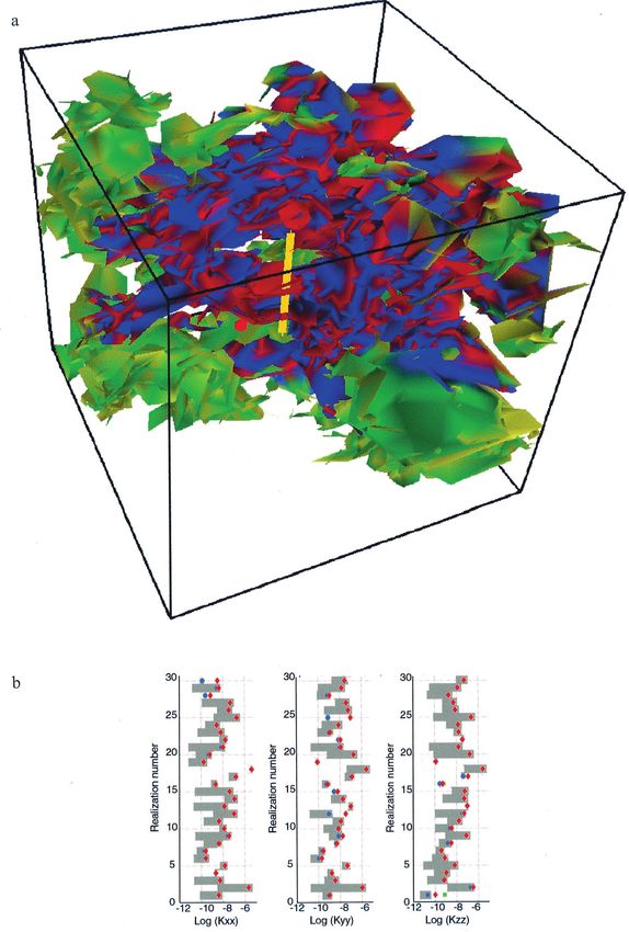
distributions in Figures 6a– 6c demonstrates the significant im- that both the data and the simulated results are based on aPlate 1. (a) Example network realization used in the 10-m scale well test simulations: Model dimensions are 30 m ⫻ 30 m ⫻ 30 m; boundary conditions are h(x, y, z, t) ⫽ 20 m at the 10-m borehole injection section and h(x, y, z, t) ⫽ 0 m at the outer boundaries. (b) Diagonal components of conductivity tensors for 30 realizations (bars indicate conductivity interval based on flux values across the two opposite surfaces, red symbols indicate tensor components based on least square fitting, blue circles indicate positive definite criterion also used for the tensors, and green squares indicate both positive definite and symmetric criterion used for the tensors).
3490                  NIEMI ET AL.: HYDRAULIC CHARACTERIZATION OF FRACTURE NETWORKS

                                                                  limited number of about 50 observations in both cases? To
                                                                  exaggerate, is the good fit just a “coincidence” explainable by
                                                                  a small number of observations? (2) Are there many other
                                                                  combinations of fracture transmissivity parameters that would
                                                                  produce equally acceptable results?
                                                                     The measured data are only one limited sample of reality. It
                                                                  is not important to capture all the details of this individual
                                                                  sample but rather to capture what can be considered repre-
                                                                  sentative taking into account the number of observations on
                                                                  which the data are based. Furthermore, it is important to find
                                                                  all the fracture transmissivity distributions that produce
                                                                  equally good fits. To investigate this, a number of Monte Carlo
                                                                  simulations with different input statistics were carried out.
                                                                  Altogether 34 sets each with 50 realizations were simulated. In
                                                                  each case the fracture log transmissivity was assumed to follow
                                                                  a Gaussian distribution, characterized by a mean and a vari-
                                                                  ance. These parameters were varied. The goodness of fit be-
                                                                  tween the modeled and the measured injection flow distribu-
                                                                  tions was determined by means of the bootstrapping method
                                                                  [e.g., Mooney and Duval, 1993]. This is a nonparametric resa-
                                                                  mpling procedure to estimate a parameter from a population
                                                                  from which we have a sample with a given number of obser-
                                                                  vations. The approach does not make any assumptions con-
                                                                  cerning the shape of the underlying distribution. The 90%,
                                                                  95%, and 99% confidence intervals determined with this
                                                                  method are shown in Figure 8 along with the measured values
                                                                  which are shown as black circles. The simulated results are
                                                                  shown as solid curves. The accepted and rejected cumulative
                                                                  curves are shown in Figures 8a and 8b, respectively. For the
                                                                  acceptance criterion the 90% confidence interval, i.e., the in-
                                                                  nermost region in Figures 8a and 8b, was used. Accepted cases
                                                                  are those for which the cumulative histogram remains entirely
                                                                  within the 90% confidence interval, i.e., inside the innermost
                                                                  shaded region. Rejected cases are those for which some part of
                                                                  the curve falls outside this region.
                                                                     Varying the standard deviation had a tendency to affect the
                                                                  slope of the curve, while changing the mean maintained the

                                                                  Figure 7. Effect of fracture transmissivity standard deviation
Figure 6. Effect of fracture storativity on simulated injection   on simulated well tests: histogram of measured data along with
flows (15-min injection period): histograms and fitted Gaussian   two simulated data sets. Simulated results are shown as Gauss-
models from 30 simulated 10-m FIL constant pressure injec-        ian fits of simulated histograms, S ⬀ 公T, in both cases.
tion tests (a) S ⬀ T, (b) S ⬀ 公T, and (c) S ⬀ 3 公T.               (Notice that the high column at Q tot ⫽ ⫺4.25 refers to all
                                                                  values at or below the equipment detection limit.)
NIEMI ET AL.: HYDRAULIC CHARACTERIZATION OF FRACTURE NETWORKS 3491
slope but moved the overall position of the curve in the hori-
zontal direction. In Figure 9 all the tested mean and standard
deviation combinations are shown on one graph. Inspection of
the results shows that a range of acceptable mean values can be
found along with a range of acceptable standard deviation
values. The preliminary transmissivity estimates based on the
Osnes et al. [1988] approach produced clearly too small flow
rates. The simulated well test curve corresponding to this pre-
liminary estimate is seen in Figure 8b as the curve in the
Figure 9. Accepted (solid circles) and rejected (open circles)
combinations for fracture transmissivity mean and standard
deviations. Results are based on stochastic fracture network
simulations of 10-m-scale injection tests. Acceptance through
comparison with measured distribution by means of bootstrap-
ping criteria (90% level) as shown in Figure 8 is indicated.
uppermost left corner of the graph. This could reflect the fact
that in the Osnes analysis the fractures are independent, which
is not a realistic presentation of a true network system. Such an
assumption may underestimate the true variability of the frac-
ture conductivities since a network can be expected to smooth
out the local heterogeneities.
5. Upscaling of Network Properties
The number of fractures in the previous network simulations
is already at the limit of reasonable computational effort.
Methods are needed to “upscale” this behavior, that is, to find
simplified presentations that reproduce the observed flow of
the detailed network. This is needed both for general site
understanding and as direct input for large-scale models. If the
upscaling of fracture networks to an “intermediate” scale (i.e.,
the scale of variability of large-scale models) shows continuum-
like behavior that can be adequately described by means of
continuum conductivity tensors, distributions of these tensors
can be used as input for large-scale stochastic continuum
Monte Carlo simulations. If the data do not meet the contin-
uum criteria, other approaches are needed such as approaches
for determining “equivalent discontinuum” properties.
5.1. Properties of Hydraulic Conductivity Tensor and
Criteria for Continuum Behavior at the “Intermediate” Scale
For anisotropic porous medium, Darcy’s law can be written as
冦冧
⭸h
Figure 8. Cumulative probabilities of measured injection
再冎 冋 册
⭸x
flows of 10-m constant pressure injection tests (circles) along qx K xx K xy K xz ⭸h
with the 90%, 95%, and 99.9% confidence intervals obtained q y ⫽ ⫺ K yx K yy K yz , (10)
with the bootstrapping method (shaded areas) and with cumu- qz K zx K zy K zz ⭸y
lative probabilities based on simulated tests: (a) accepted and ⭸h
(b) rejected cases. ⭸z3492 NIEMI ET AL.: HYDRAULIC CHARACTERIZATION OF FRACTURE NETWORKS
where q i are the components of the specific discharge or the simulated from three different directions. The direction is var-
Darcy velocity vector, K ij are the components of the hydraulic ied so that each pair of opposing faces of the cube, in turn, is
conductivity tensor, and ⭸h/⭸i are the components of the hy- assigned the maximum head difference.
draulic gradient vector. For a homogeneous porous medium For hydraulic properties the calibrated values from section
the hydraulic conductivity tensor has to be symmetric with 4.4 were used. More precisely, values falling in the middle of
respect to the diagonal (i.e., K xy ⫽ K yx , K zx ⫽ K xz , and K yz ⫽ the acceptable region in Figure 9 are selected, with a mean of
K zy ), and it can be transformed into a diagonal form by a log transmissivity m ⫽ ⫺14.6 and standard deviation ⫽ 3.6.
rotation of the coordinate axes. Anisotropic porous media fol- As these simulations are steady state, no values are needed for
low this concept. Graphically, the tensor plots as an ellipsoid in fracture storativities. The same 30 network realizations are
three dimensions and as an ellipse in two dimensions, with the used as before, but the inactive fractures to be removed are
major and minor axes corresponding to directions of minimum readjusted according to the new problem specifications. In the
and maximum permeability. When looking at whether a frac- calibration simulations the fractures that were not connected
ture network behaves as a continuum, the properties of the to the borehole were removed, as they did not influence the
conductivity ellipse have been used as a criterion [Long et al., flow. Here they are not excluded. However, isolated fractures
1982; Cacas et al., 1990; National Research Council, 1996]. The that had no connection to any of the boundaries, including
conductivity ellipse is then determined by simulating the steady connections through other fractures, are excluded. Such frac-
state flow through a network block and by determining the tures are completely isolated in terms of the overall block
effective hydraulic conductivity based on the one-dimensional conductivity and do not influence the solution physically. They
form of Darcy’s law according to the imposed hydraulic gradi- do, however, create problems for the iterative solution procedure.
ent and the observed total flow. The direction of the main flow With these specifications the flow field is simulated for 30
is varied with respect to the network and the conductivity (or network realizations altogether, with three simulations corre-
more precisely 1/公K); for each direction is plotted as a func- sponding to the three main directions of flow for each. The
tion of the rotational angle. The closer to a perfect ellipse this Darcy flux inside the simulation cube (q) can be determined
plot is, the closer to a continuum the system behaves. There is based on the observed flow rates through the six faces of the
no guarantee that fractured media will behave like this. Long et cube (Qⴕ) according to the equation
al. [1982] looked at different fracture systems in two dimen-
sions and found that a perfect ellipse was, indeed, often not aq ⫽ Qⴕ, (11)
found for realistic fracture systems. The factors favoring the where the Darcy flux is q ⫽ {q x , q y , q z }, Qⴕ ⫽ {Q 1 /A 1 ,
continuum-type behavior were high fracture density and mixed Q 2 /A 2 䡠 䡠 䡠 Q 6 /A 6 }, with A I being the cross-sectional areas of
directions of the fracture orientations. Cacas et al. [1990] the block surfaces and Q i being the flow rates through them.
looked at the permeability ellipse of fracture network data A is the coefficient matrix A ⫽ {a j k } ( j ⫽ 1, 䡠 䡠 䡠 , 6 and k ⫽
from Fanay-Augeres mine and found relatively well behaving x, y, z), where a jx , a jy , and a jz represent the components of
ellipse-like shapes. The Fanay-Aurgeres data were character- the unit vector normal to surface j.
ized by a relatively high overall conductivity and well- When simulation directions are selected to coincide with x,
connected networks and came from relatively shallow depths y, and z, the (11) has three unknowns (the components of
of a few hundred meters. It is of interest to note, however, that vector q) and six equations corresponding to flow through each
the model failed to reproduce the lack of hydraulic intercon- of the block surfaces. This means that, for example, for the
nection observed at the site. The reason for this has been component q x we have two estimates corresponding to the two
proposed to be the fact that the network model was based on flow rates Q i through the two opposite faces of the cube per-
apparent rather than conductive fracture geometry [National pendicular to x direction. If the medium were a perfect homo-
Research Council, 1996]. geneous porous medium, these should be equal to each other.
Another criterion for continuum behavior, which actually In the case of heterogeneity and spatially variable q x inside the
follows from the ellipse/ellipsoid requirement, is that the flow cube, the two values differ. How much they differ can be taken
coming in through one face of a block is equal to that going out as a measure of deviation from the homogeneous porous me-
through the opposite face. The three-dimensional networks dium behavior.
studied here are computationally extensive. Therefore, as a Knowing the components of the Darcy flux based on (11),
starting point, we use this criterion to evaluate the continuum- the components of the permeability tensor can be solved from
like character of the networks. This allows the use of somewhat (10). If no assumptions are made concerning the symmetric
fewer simulation directions per realization than would be re- properties of the tensor, (10) has nine unknowns and three
quired when determining the full ellipsoid. equations. Therefore a minimum of three sets of simulations,
corresponding to three different sets of hydraulic gradient, is
5.2. Simulations for Block Conductivities
needed to solve the nine components of the conductivity tensor.
The objective of these simulations is to look at the validity of
the continuum behavior of the network blocks and to deter- 5.3. Continuum Characteristics and Tensor Properties
mine the equivalent continuum conductivities that would re- Plate 1b shows the calculated diagonal components of the
produce their hydraulic behavior. The calibrated 30-m fracture conductivity tensors for the 30 realizations. These are marked
network blocks were used in the simulations. The steady state with three different symbols, depending on the mathematical
flow through the blocks is simulated by imposing constant criteria used in their determination. These will be discussed
specified head boundary conditions on opposite sides of the later. More importantly, Plate 1b also shows the conductivities
cube along with linearly varying specified head boundaries determined based on the flow through each individual face of
along the other four sides. Consequently, the external potential the simulation block. According to the notation of Long et al.
gradient is as constant as possible, as required by Darcy’s law [1982] we call this conductivity K g , i.e., hydraulic conductivity
and continuum approximation. For each realization the flow is in the direction of the imposed gradient,NIEMI ET AL.: HYDRAULIC CHARACTERIZATION OF FRACTURE NETWORKS 3493
K gi ⫽ Q i/共⌬hA i兲 i ⫽ 1, . . . , 6, (12)
where ⌬h is the imposed hydraulic gradient. For each main
flow direction, there are two faces yielding two values for this
estimate. These are shown as the ends of the grey bars in Plate
1b. The closer the values are to each other, the shorter the bar
is. For continuum approximation to be valid, the two values of
K g should be equal. Inspection of the K g values in Plate 1b
shows that for the present data the K g conductivities differ in
most cases quite significantly, often by orders of magnitude.
This indicates that the behavior of the cubes cannot be well
presented with a continuum tensor, and the use of a continuum
tensor is not justified. For demonstrative purposes these are,
however, also given in Plate 1b. Values indicated with red are
determined based on the three simulations and (10) and (11)
without any constraints for the characteristics of the resulting
matrix. The blue symbols correspond to the corresponding
values when the matrices were in addition required to be pos-
itive definite, and the green square symbols correspond to the
case where they were required to be symmetric as well as
positive definite.
Figure 10. Conductivity “ellipsoid” (1/公K) for realization
Inspection of the results in Plate 1b indicates the following: number (a) 4 and (b) 29 in Plate 1b. (Notice that the presen-
(1) There appears to be no clear anisotropy; that is, the con- tation in Figure 10b is partly “truncated” as otherwise 1/公K
ductivity values are of the same order of magnitude in all would become very large when K becomes very small.)
directions. (2) In most cases, there is very little difference
between the diagonal terms of the three different types of
matrices, and the different symbols fall on top of each other. 6. Comparison of Fracture Network–Based
(3) The calculated values of the diagonal terms are always very Conductivities With Conductivities
close to the upper one of the two K g values. This is an artefact From Well Tests
of both the solution method and the fact that the two values of It is of interest to compare the results of the network sim-
the Darcy flux corresponding to the two opposite faces of the ulations to the well test results of the same scale. In this case
cube differ so much. The set of the six equations (equation these are the constant-pressure injection tests with 30-m fixed-
(11)) was solved with the method of least squares. In doing so, interval testing length. From these data the hydraulic conduc-
one searches for the solution by minimizing the sum of squared tivities have been determined with different standard interpre-
differences. For example, in the case of Darcy flux in the x tation formulae, using the method by Jacob and Lohman
direction the quantity (q x ⫺ Q x1 /A x1 ) 2 ⫹ (q x ⫺ Q x2 /A x2 ) 2 [1952], the Horner method [Uraiet and Raghavan, 1980], and
is minimized. When doing so with values that differ even by the method by Moye [1967]. All of these standard interpreta-
orders of magnitude, the higher value is automatically over- tion methods assume continuum behavior with radial or radial-
emphasized. to-spherical flow geometry. In “classical” stochastic continuum
An example of a conductivity ellipsoid corresponding to a analysis [Neuman, 1987; Gomez-Hernandez and Gorelick, 1989;
continuum-like behavior with a small difference between the Tsang et al., 1996] such data are used directly as the basis for
K g is given in Figure 10a. This is realization number 4 in Plate generating input conductivity distributions for Monte Carlo
1b. An example with large deviation from this behavior, i.e., type simulations.
realization number 29 in Plate 1b, is given in Figure 10b. The information from the well tests can be seen as repre-
Only three simulation directions were used. It is possible senting a one-dimensional sample of the rock conductive prop-
erties along the borehole. It is of interest to see how well it
that these happen to present especially heterogeneous direc-
corresponds to the conductivities and resulting flow rates
tions not representative of the medium. Then choosing a finer
through two-dimensional surfaces in heterogeneous systems.
angle of rotation would result in a more ellipsoid-like appear-
In homogeneous systems these values are equal to one an-
ance in the heterogeneous realizations. This is, however, quite
other.
unlikely as we already have 3 ⫻ 30 samples of the K g perme-
Although the present data do not appear to be well approx-
abilities in the selected scale, the vast majority of them indi- imated by a continuum conductivity tensor, the K g values in
cating heterogeneous behavior. From the above results it is Plate 1b can be taken as samples of some type of “block
apparent that the least square approximation used to average interface” conductivity in the 30-m scale. Conductivity then
the Darcy flux through the cube is also not suitable. Another refers simply to a proportionality coefficient linking the im-
averaging method could be chosen that does not so apparently posed hydraulic gradient, flow rate, and surface area. These
overemphasize the effect of higher flux. The overall large dif- values were plotted as cumulative histograms by taking the K g
ference between the K g values at opposite ends of the cube, values for each computational direction as an independent
however, indicates that the continuum approximation is not a sample. For conductivity perpendicular to the x direction all 60
good presentation for the data and scale in question in general. values (both ends of the bars) in the first column in Plate 1b are
Therefore alternative averaging methods were not investigated combined into one data set. The resulting cumulative histo-
further. gram is shown in Figure 11a along with the correspondingYou can also read