Ideas and perspectives: is shale gas a major driver of recent increase in global atmospheric methane?
←
→
Page content transcription
If your browser does not render page correctly, please read the page content below
Biogeosciences, 16, 3033–3046, 2019
https://doi.org/10.5194/bg-16-3033-2019
© Author(s) 2019. This work is distributed under
the Creative Commons Attribution 4.0 License.

Ideas and perspectives: is shale gas a major driver of recent increase
in global atmospheric methane?
Robert W. Howarth
Department of Ecology and Evolutionary Biology, Cornell University, Ithaca, NY 14853, USA

Correspondence: Robert W. Howarth (howarth@cornell.edu)

Received: 10 April 2019 – Discussion started: 23 April 2019
Revised: 11 July 2019 – Accepted: 12 July 2019 – Published: 14 August 2019

Abstract. Methane has been rising rapidly in the atmosphere     Convention on Climate Change (UNFCCC) COP21 target of
over the past decade, contributing to global climate change.    keeping the planet well below 2 ◦ C above the pre-industrial
Unlike the late 20th century when the rise in atmospheric       baseline (IPCC, 2018). Methane also contributes to the for-
methane was accompanied by an enrichment in the heav-           mation of ground-level ozone, with large adverse conse-
ier carbon stable isotope (13 C) of methane, methane in re-     quences for human health and agriculture. Considering these
cent years has become more depleted in 13 C. This depletion     effects as well as climate change, Shindell (2015) estimated
has been widely interpreted as indicating a primarily bio-      that the social cost of methane is 40 to 100 times greater than
genic source for the increased methane. Here we show that       that for carbon dioxide: USD 2700 per ton for methane com-
part of the change may instead be associated with emissions     pared to USD 27 per ton for carbon dioxide when calculated
from shale-gas and shale-oil development. Previous studies      with a 5 % discount rate and USD 6000 per ton for methane
have not explicitly considered shale gas, even though most      compared to USD 150 per ton for carbon dioxide when cal-
of the increase in natural gas production globally over the     culated with a 1.4 % discount rate.
past decade is from shale gas. The methane in shale gas is         Atmospheric methane levels rose steadily during the last
somewhat depleted in 13 C relative to conventional natural      few decades of the 20th century before leveling off for
gas. Correcting earlier analyses for this difference, we con-   the first decade of the 21st century. Since 2008, how-
clude that shale-gas production in North America over the       ever, methane concentrations have again been rising rapidly
past decade may have contributed more than half of all of the   (Fig. 1a). This increase, if it continues in coming decades,
increased emissions from fossil fuels globally and approx-      will significantly increase global warming and undercut ef-
imately one-third of the total increased emissions from all     forts to reach the COP21 target (Nisbet et al., 2019). The
sources globally over the past decade.                          total atmospheric flux of methane for the period 2008–2014
                                                                was ∼ 24.7 Tg per year greater than for the 2000–2007 pe-
                                                                riod (Worden et al., 2017), an increase of 7 % in global
                                                                human-caused methane emissions. The change in the sta-
1   Introduction                                                ble carbon δ 13 C ratio of methane in the atmosphere over
                                                                the past 35 years is striking and seems clearly related to the
Methane is the second most important greenhouse gas behind      change in the methane concentration (Fig. 1b). For the final
carbon dioxide causing global climate change, contributing      20 years of the 20th century, as atmospheric methane con-
approximately 1 W m−2 to warming when indirect effects          centrations rose, the isotopic composition became more en-
are included compared to 1.66 W m−2 for carbon dioxide          riched in the heavier stable isotope of carbon, 13 C, relative
(IPCC, 2013). Unlike carbon dioxide, the climate system         to the lighter and more abundant isotope, 12 C, resulting in a
responds quickly to changes in methane emissions, and re-       less negative δ 13 C signal. The isotopic composition remained
ducing methane emissions could provide an opportunity to        constant from 1998 to 2008, when the atmospheric concen-
immediately slow the rate of global warming (Shindell et        tration was constant. And the isotopic composition has be-
al., 2012) and perhaps meet the United Nations Framework

Published by Copernicus Publications on behalf of the European Geosciences Union.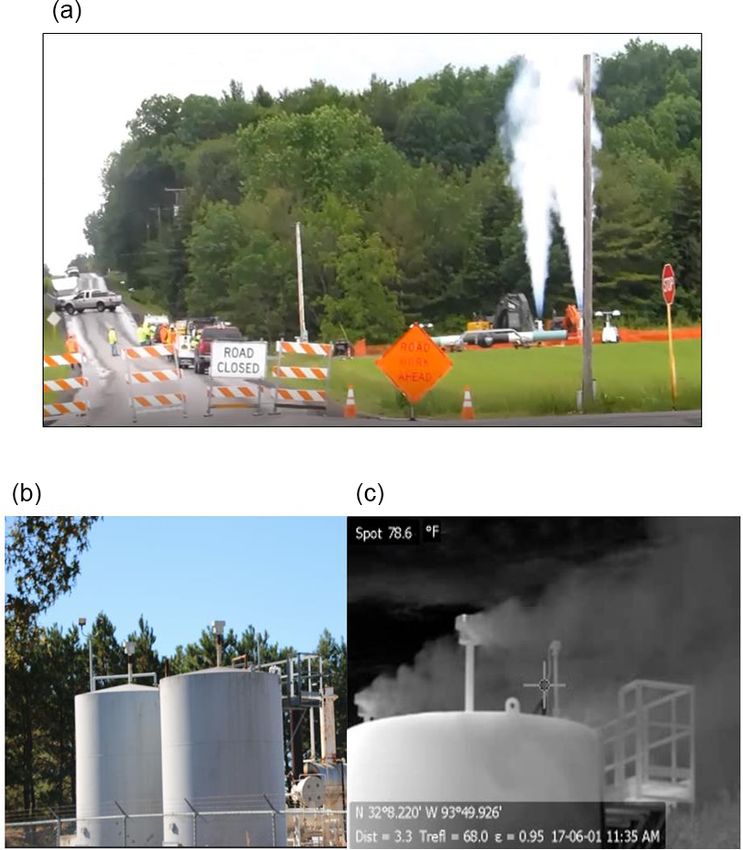
3034 R. W. Howarth: Shale gas and global methane
a larger and more comprehensive data set for the δ 13 C values
of methane emission sources. They too concluded that fossil-
fuel emissions have likely decreased during this century and
that biogenic emissions are the probable cause of any recent
increase in global methane emissions.
2 Sensitivity of emission models based on δ 13 C in
methane to biomass burning
Model analyses that use δ 13 C methane data to infer emis-
sion sources are highly sensitive to changes in the rate of
biomass burning: although biomass burning is a relatively
small contributor to global methane emissions, those emis-
sions are quite enriched in 13 C relative to the atmospheric
methane signal (Rice et al., 2016; Sherwood et al., 2017).
Both Schaefer et al. (2016) and Schwietzke et al. (2016)
assumed that biomass burning had been constant in recent
years. However, Worden et al. (2017) estimated that biomass
burning globally went down for the period 2007–2014 com-
pared to 2001–2006, resulting in decreased methane emis-
sions of 3.7 Tg per year (±1.4 Tg per year) and contributing
to a lower δ 13 C for atmospheric methane. Using the data set
of Schwietzke et al. (2016) for δ 13 C values of methane emis-
sion sources, but including changes in biomass burning over
time, Worden et al. (2017) concluded that the recent increase
in methane emissions was likely driven more by fossil fu-
els than by biogenic sources, with an increase of 16.4 Tg per
year from fossil fuels (±3.6 Tg per year) compared to an in-
Figure 1. (a) Global increase in atmospheric methane between crease of 12 Tg per year from biogenic sources (±2.5 Tg per
1980 and 2015. (b) Change in δ 13 C value of atmospheric methane year) when comparing 2007–2014 to 2001–2006.
globally between 1980 and 2015. Both adapted from Schaefer et Clearly global models for partitioning methane sources
al. (2016). based on the δ 13 C approach are sensitive to assumptions
about seemingly small terms such as decreases in biomass
burning. In this paper, we explore for the first time another as-
sumption: that the global increase in shale-gas development
come lighter (depleted in 13 C, more negative δ 13 C) since
may have caused some of the depletion of 13 C in the global
2009, as atmospheric methane concentrations have been ris-
average methane observed over the past decade. Shale-gas
ing again (Schaefer et al., 2016; Nisbet et al., 2016). Since
emissions were not explicitly considered in the models pre-
biogenic sources of methane are lighter than the methane
sented by Schaefer et al. (2016) and Worden et al. (2017)
released from fossil-fuel emissions, Schaefer et al. (2016)
and were explicitly excluded in the analysis of Schwietzke et
concluded that the increase in atmospheric methane in the
al. (2016).
late 20th century was due to increasing emissions from fos-
sil fuels but that the increase in methane since 2006 is due
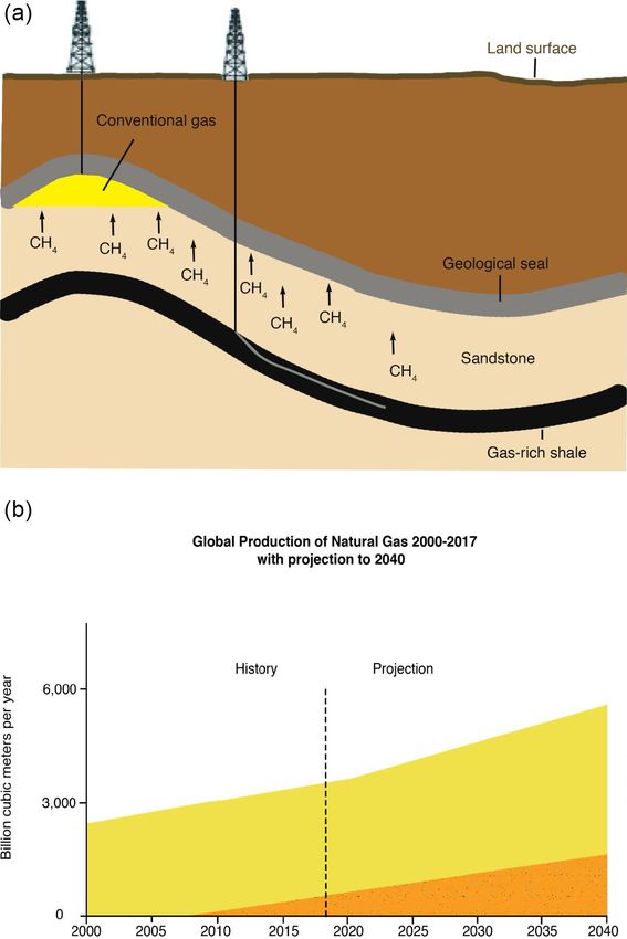
to biogenic sources, most likely tropical wetlands, rice cul- 3 What is shale gas?
ture, or animal agriculture. Their model results indicated that
fossil-fuel sources have remained flat or decreased globally Shale gas is a form of unconventional natural gas (mostly
since 2006, playing no major role in the recent atmospheric methane) held tightly in shale-rock formations. Conventional
rise of methane. Schaefer et al. (2016) noted that their con- natural gas, the dominant form of natural gas produced dur-
clusion contradicted many reports of increased emissions ing the 20th century, is composed largely of methane that
from fossil-fuel sources over this time and stated that their migrated upward from the underlying sources such as shale
conclusion was “unexpected, given the recent boom in un- rock over geological time, becoming trapped under a geo-
conventional gas production and reported resurgence in coal logical seal (Fig. 2a). Until this century, shale gas was not
mining and the Asian economy”. Six months after the Schae- commercially developable. The use of a new combination
fer et al. (2016) study was published in Science, Schwietzke of technologies in the 21st century – high-precision direc-
et al. (2016) presented a similar analysis in Nature that used tional drilling, high-volume hydraulic fracturing, and clus-
Biogeosciences, 16, 3033–3046, 2019 www.biogeosciences.net/16/3033/2019/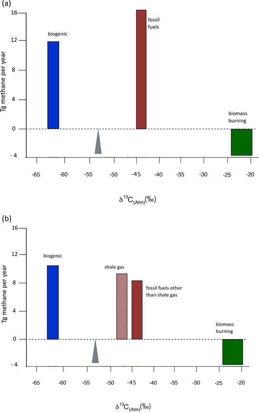
R. W. Howarth: Shale gas and global methane                                                                                    3035

                                                                         Several studies have suggested that the δ 13 C signal of
                                                                      methane from shale gas can often be lighter (more depleted
                                                                      in 13 C) than that from conventional natural gas (Golding et
                                                                      al., 2013; Hao and Zou, 2013; Turner et al., 2017; Botner
                                                                      et al., 2018). This should not be surprising. In the case of
                                                                      conventional gas, the methane has migrated over geological
                                                                      time frames from the shale and other source rocks through
                                                                      permeable strata until trapped below a seal (Fig. 2a). Dur-
                                                                      ing this migration, some of the methane can be oxidized both
                                                                      by bacteria, perhaps using iron (III) or sulfate as the source
                                                                      of the oxidizing power, and by thermochemical sulfate re-
                                                                      duction (Whelan et al., 1986; Burruss and Laughrey, 2010;
                                                                      Rooze et al., 2016). This partial oxidation fractionates the
                                                                      methane by preferentially consuming the lighter 12 C isotope
                                                                      and gradually enriching the remaining methane in 13 C (Hao
                                                                      and Zou, 2013; Baldassare et al., 2014), resulting in a δ 13 C
                                                                      signal that is less negative. The methane in shales, on the
                                                                      other hand, is tightly held in the highly reducing rock for-
                                                                      mation and therefore very unlikely to have been subject to
                                                                      oxidation and the resulting fractionation. The expectation,
                                                                      therefore, is that methane in conventional natural gas should
                                                                      be heavier and less depleted in 13 C than the methane in shale
                                                                      gas.

                                                                      4   Calculating the effect of 13 C signal of shale gas on
                                                                          emission sources: conceptual framework

                                                                      To explore the contribution of methane emissions from shale
                                                                      gas, we build on the analysis of Worden et al. (2017). Fig-
                                                                      ure 3a shows the δ 13 C values used by them as well as their
                                                                      mean estimates for changes in emissions since 2008 (as they
Figure 2. (a) Schematic comparing shale gas and conventional nat-     estimated using the δ 13 C data of Schwietzke et al., 2016).
ural gas. For conventional natural gas, methane migrates from the     Figure 3a represents a weighting for the change in emis-
shale through semipermeable formations over geological time, be-
                                                                      sions (y axis) and the δ 13 C values of those emissions (x
coming trapped under a geological seal. Shale gas is methane that
                                                                      axis) by individual sources. Our addition is to separately con-
remained in the shale formation and is released through the com-
bined technologies of high-precision directional drilling and high-   sider shale-gas emissions, recognizing that methane emis-
volume hydraulic fracturing. (b) Global production of shale gas and   sions from shale gas are more depleted in 13 C than for con-
other forms of natural gas from 2000 to 2017, with projections into   ventional natural gas or other fossil fuels as considered by
the future from EIA (2016). Redrawn from EIA (2016) with data         Worden et al. (2017). For this analysis, we accept that net to-
from IEA (2017).                                                      tal emissions have increased by 24.7 Tg per year (±14.0 Tg
                                                                      per year) since 2007, driven by an increase of ∼ 28.4 Tg per
                                                                      year for the sum of biogenic emissions and emissions from
                                                                      fossil fuels and a decrease of ∼ 3.7 Tg per year for emissions
                                                                      from biomass burning (Worden et al., 2017).
tered multi-well drilling pads – has changed this. In re-
                                                                         We start with Eq. (1), which expresses the findings of Wor-
cent years, global shale-gas production has exploded 14-fold,
                                                                      den et al. (2017):
from 31 billion cubic meters per year in 2005 to 435 billion
cubic meters per year in 2015 (Fig. 2b), with 89 % of this            BW + FFW = 28.4 Tg yr−1 ,                                   (1)
production in the United States and 10 % in western Canada
                                                                      where BW and FFW are the estimates from Worden et
(EIA, 2016). Shale gas accounted for 63 % of the total in-
                                                                      al. (2017) for the increase respectively in biogenic emissions
crease in natural gas production globally over this time pe-
                                                                      and fossil-fuel emissions of methane globally since 2007.
riod (EIA, 2016; IEA, 2017). The US Department of Energy
                                                                      Equation (2) explicitly considers methane emissions from
predicts rapid further growth in shale-gas production glob-
                                                                      shale gas:
ally, reaching 1500 billion cubic meters per year by 2040
(EIA, 2016; Fig. 2b).                                                 BN + FFN + SG = 28.4 Tg yr−1 ,                              (2)

www.biogeosciences.net/16/3033/2019/                                                         Biogeosciences, 16, 3033–3046, 2019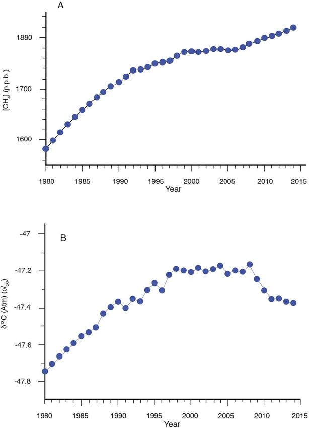
3036                                                                                      R. W. Howarth: Shale gas and global methane

Figure 3. (a) On the x axis, δ 13 C values for methane from biogenic sources, fossil fuel, and biomass burning as presented in Worden et
al. (2017) for values from Schwietzke et al. (2016); width of horizontal bars represents the 95 % confidence limits for these values. Triangle
indicates the flux-weighted mean input of methane to the atmosphere. The y axis shows mean estimates from Worden et al. (2017) for
the increase and decrease in methane emissions from particular sources since 2007 as calculated using the δ 13 C values of Schwietzke et
al. (2016). (b) On the x axis, δ 13 C values as in Fig. 3a, except the value for fossil fuels does not include shale gas and a separate estimate for
shale-gas value is included (see text). The y axis indicates estimates developed in this paper for the increase or decrease in methane emissions
since 2008.

Biogeosciences, 16, 3033–3046, 2019                                                                 www.biogeosciences.net/16/3033/2019/
R. W. Howarth: Shale gas and global methane                                                                                 3037

where BN is our new estimate for the increase in the biogenic      al., 2012). Note that in the Barnett shale region, Texas, the
fluxes since 2007, FFN is our new estimate for the increase        δ 13 C ratio for methane emitted to the atmosphere (−46.5 ‰;
in fossil-fuel emissions other than shale gas since 2007, and      Townsend-Small et al., 2015) is more depleted than the av-
SG is our estimate for emissions from shale gas since 2007.        erage for wells reported in the Sherwood et al. (2017) data
Subtracting Eq. (2) from Eq. (1),                                  set: −44.8 ‰ for “group 2A and 2B” wells and −38.5 ‰ for
                                                                   “group 1” wells (Rodriguez and Philp, 2010) and a −41.1 ‰
(BW − BN ) + (FFW − FFN ) − SG = 0.                         (3)    average value (Zumberge et al., 2012). For our analysis, we
                                                                   use the mean of the δ 13 C ratio (−46.9 ‰) from three stud-
   Equation (4) builds on Eq. (3) and reweights the informa-
                                                                   ies where the methane clearly came from horizontal, high-
tion in Fig. 3a for the difference between most fossil fuels
                                                                   volume fractured shale wells: −47.0 ‰ for Bakken shale,
and shale gas, multiplying global mass fluxes for each source
                                                                   North Dakota (Schoell et al., 2011), −46.5 ‰ for Barnett
by the difference between the δ 13 C ratio of each source and
                                                                   shale, Texas (Townsend-Small et al., 2015), and −47.3 ‰
the flux-weighted mean for all sources:
                                                                   for Utica shale, Ohio (Botner et al., 2018). Note that sev-

  (BW − BN ) · DB−A + (FFW − FFN ) · DFF−A
                                                                  eral studies have reported mean δ 13 C ratios for methane
                                                                   from organic-rich shales that are more depleted in 13 C (more
  − (SG · DSG−A ) = 0,                                      (4)    negative) than this: −50.7 (Martini et al., 1998) for Antrim
                                                                   shale, Michigan, −53.3 (McIntosh et al., 2002) and −51.1
whereDB−A ,DFF−A , and DSG−A are the differences in the
                                                                   (Schlegel et al., 2011) for New Albany shale, Illinois, and
δ 13 C ratio of biogenic emissions, fossil fuels, and shale
                                                                   −49.3 (Osborn and McIntosh, 2010) for a Devonian shale
gas compared to the flux-weighted mean δ 13 C ratio for all
                                                                   in Ohio. However, these shales are not typical of the major
sources (A). The x axis of Fig. 3b shows the δ 13 C for each
                                                                   shale plays supporting the huge increase in gas production
source; note that the y axis is the estimate of the change in
                                                                   over the past decade.
emissions for each of the sources that we derive below. Next,
                                                                      The average δ 13 C ratio for methane in the atmosphere (A)
we multiply both sides of Eq. (3) byDB−A ,
                                                                   in 2005 was −47.2 ‰ (Schaefer et al., 2016), which reflects
                                                                   a flux-weighted mean input of methane with a δ 13 C ratio of

  (BW − BN ) · (DB−A ) + (FFW − FFN ) · DB−A
                                                                   −53.5 ‰. This flux-weighted mean value is approximately
  − SG · (DB−A ) = 0.                                       (5)
                                                                   6.3 ‰ more depleted in 13 C because of fractionation during
  Subtracting Eq. (5) from Eq. (4),                                the oxidation of methane in the atmosphere (Schwietzke et
                                                                 al., 2016; Sherwood et al., 2017). In our analysis, we use this
 (FFW − FFN ) · (DFF−A − DB−A )                                    flux-weighted mean value of −53.5 ‰. Therefore, the mean

  − SG · (DSG−A − DB−A ) = 0.                               (6)    value for DFF−A is −9.5 ‰, the value for DB−A is 9.0 ‰, and
                                                                   the value for DSG−A is −6.6 ‰ (Fig. 3b). Substituting these
  Rearranging Eq. (6) to solve for SG,                             values into Eq. (7), we see that

SG = (FFW − FFN ) · (DFF−A − DB−A ) /                              SG = −1.19 · FFN + 19.4.                                   (8)

  (DSG−A − DB−A ) .                                         (7)
                                                                   5   Estimating increased methane fluxes for coal, oil, and
   Note that from Worden et al. (2017), FFW is 16.4 Tg per             natural gas
year.
   Although our expectation is that the methane in shale gas       Next, we estimate the likely contributions from coal and oil
is depleted in 13 C relative to conventional natural gas, the      to the increased methane emissions over the past decade. We
δ 13 C ratios for the methane in both conventional gas reser-      estimate the increase in methane emissions from coal be-
voirs and in shale gas vary substantially, changing with the       tween 2006 and 2016 to be 1.3 Tg per year, based on the rise
maturity of the gas and several other factors (Golding et al.,     in global coal production of 27 %, with almost all of this due
2013; Hao and Zou, 2013; Tilley and Muehlenbachs, 2013).           to surface-mined coal in China (IEA, 2008, 2017) and us-
The large data set of Sherwood et al. (2017) suggests no sys-      ing a well-accepted emission factor of 870 g methane per ton
tematic difference between the average ratio for shale gas and     of surface-mined coal (Howarth et al., 2011). Methane emis-
the average for conventional gas. However, some of the data        sions from surface-mined coal tend to be low, as much of the
listed as shale gas in that data set are actually for methane      methane that was once associated with the coal has degassed
that has migrated from shale to reservoirs (Tilley et al., 2011)   over geological time. This estimate is very close to the 1.1 Tg
and therefore may have been partially oxidized and fraction-       per year increase from coal emissions in China between 2009
ated (Hao and Zou, 2013). In other cases, the data appear          and 2015 as estimated based on satellite observations (Miller
to come both from conventional vertical wells and shale-           et al., 2019). For oil, global production increased by 9.6 %
gas horizontal wells in the same region, making interpreta-        (IEA, 2008, 2017), thereby increasing methane emissions by
tion ambiguous (Rodriguez and Philp, 2010; Zumberge et             approximately 1.6 Tg per year (using emission factors from

www.biogeosciences.net/16/3033/2019/                                                      Biogeosciences, 16, 3033–3046, 2019
3038 R. W. Howarth: Shale gas and global methane
NETL 2008; as detailed in Howarth et al., 2011). Therefore, et al. (2017), although our estimate for fossil fuels is larger
of the increase in 28.4 Tg per year from fossil fuels plus bio- and our estimate for biogenic fluxes lower than their esti-
genic sources since 2005 (see discussion above), we estimate mates. On the other hand, comparing emissions for the 2003–
2.9 Tg per year to be from increased emissions from coal and 2013 period with those from the late 20th century, Schwi-
oil, leaving an increase of approximately 25.5 Tg per year etzke et al. (2016) concluded that biogenic emissions had
from natural gas (including shale gas) plus biogenic sources. risen by ∼ 27 Tg per year, while fossil-fuel emissions had
As noted above, shale gas accounted for 63 % of the global decreased by ∼ 18 Tg per year. And Schaefer et al. (2016)
increase in all natural gas production between 2005 and 2015 concluded that increased methane emissions since 2006 have
(EIA, 2016; IEA, 2017). If we make the simplifying assump- been “predominantly biogenic” and that fossil-fuel emissions
tion that for both shale gas and conventional natural gas, likely have fallen.
emissions are equal as a percentage of the gas produced, then We estimate that shale gas has contributed 33 % of the
global increase in all methane emissions in recent years
SG = 0.63 · TG, (9) (Table 1). Since virtually all shale-gas development glob-
ally through 2015 occurred in North America (mostly in the
and United States but also western Canada), we conclude that
at least 33 % of the increase in methane fluxes came from
CG = 0.37 · TG, (10)
North America. This is consistent with the work of Turner
where TG is total increase in emissions from all natural gas. et al. (2016), who used satellite data to conclude that 30 %
Note that we test this assumption later in our sensitivity anal- to 60 % of the global increase in methane emissions between
yses, since some research indicates that emissions from shale 2002 and 2014 came from the United States. On the other
gas are higher than for conventional gas as a percentage of hand, Nisbet et al. (2016, 2019) used monitoring data to in-
gas production. Rearranging Eq. (9) for TG and substituting fer spatial changes in methane emissions over time and em-
into Eq. (10), phasized that much of the increase in recent years originated
in the tropics and Southern Hemisphere, although they noted
CG = 0.37 · (SG/0.63), or CG = 0.59 · SG. (11) that the northern temperate latitude played a major role in
the large increase in emissions in 2014 (Nisbet et al., 2019),
FFN is the sum of CG (0.59 · SG) plus the emissions from oil a time of major increase in shale-gas development (EIA,
and coal (2.9 Tg per year), or 2016). While our estimate for increased emissions from fos-
sil fuels is only marginally greater than that of the Worden
FFN = (0.59 · SG) + 2.9. (12) et al. (2017) paper upon which we build our analysis, we
demonstrate the importance of shale gas as a major part of
Substituting Eq. (12) into Eq. (8) and solving for SG, we
these increased fossil-fuel emissions and thereby explicitly
estimate that the increase in shale-gas emissions between
link the increased emissions to North America.
2005 and 2015 was 9.4 Tg per year (Table 1; Fig. 3b). From
Our estimate of increased emissions of 9.4 Tg per year
Eq. (11), increased emissions from conventional natural gas
from shale-gas development is quite reasonable in light of the
are then estimated to be 5.5 Tg per year, emissions from
growing body of evidence from measurements made at local
all natural gas (shale plus conventional) are estimated to be
to regional scales. Between 2005 and 2015, global shale-gas
14.9 Tg per year, and emissions from all fossil fuels (includ-
production rose by 404 billion cubic meters per year (Fig. 2b;
ing coal and oil) are estimated to be 17.8 Tg per year. From
EIA, 2016). Assuming that 93 % of natural gas is composed
Eq. (3), increased emissions from biogenic sources are es-
of methane (Schneising et al., 2014), our estimate of the in-
timated to be 10.6 Tg per year. While the biogenic sources
crease in methane emissions from shale gas represents 3.5 %
are important, the increase in fossil-fuel emissions has been
of the shale-gas production (270 Tg per year of methane pro-
greater, and shale gas makes up more than half of these in-
duced from shale-gas operations on average in 2015). This
creased fossil-fuel emissions.
estimate of 3.5 % (based on global change in the 13 C con-
tent of methane) represents full life-cycle emissions, includ-
6 Comparison with prior estimates ing those from the gas well site, transportation, processing,
storage systems, and final distribution to customers. Our es-
Our best estimate for the increase in methane emissions from timate is well within the range reported in several recent stud-
all fossil fuels since 2008 (shale gas, conventional natural ies for shale gas and in fact is at the low end for many (but
gas, coal, and oil) of 17.8 Tg per year is 9 % larger than the not all) of these studies (Howarth et al., 2011; Pétron et al.,
mean estimate of Worden et al. (2017) of 16.4 Tg per year 2014; Karion et al., 2013; Caulton et al., 2014; Schneising et
(Table 1). Our estimate for the increased emissions from bio- al., 2014; Howarth, 2014). Alvarez et al. (2018) recently pre-
genic sources, 10.6 Tg per year, is 12 % lower than the Wor- sented a summary estimate for natural gas emissions in the
den et al. (2017) estimate of 12 Tg per year (Table 1). Thus, United States (both conventional and shale gas) of 2.3 % us-
our estimates are not greatly different from those of Worden ing bottom-up, facility-based data. However, they noted that
Biogeosciences, 16, 3033–3046, 2019 www.biogeosciences.net/16/3033/2019/R. W. Howarth: Shale gas and global methane 3039
Table 1. Estimates for sources of increased or decreased methane emissions to the atmosphere in recent years (teragrams per year). All values
are positive, except as specified.
This studya Worden et al.b Schwietzke et al.c
(2017) (2016)
All fossil fuels 17.8 16.4 Negative ∼ 18
(±3.6)
– Shale gas 9.4
– Conventional gas 5.5
– Oil 1.6
– Coal 1.3
Biogenic sources 10.6 12.0 ∼ 27
(±2.5)
a Time period is 2008–2014 compared to 2000–2007. b Time period is 2008–2014 compared to
2000–2007, using the Schwietzke et al. (2016) data set with values from their Fig. 4 and assuming a
decrease in biomass burning of 3.7 Tg per year. Uncertainty is as shown in original publication.
c Time period is for 2003–2013 compared to 1985–2002, with values from their Fig. 2b.
Uncertainties are large, and only mean differences shown here.
Table 2. Exploration of sensitivity to assumptions for estimates of increase in global methane emissions in recent years (teragrams per year).
Base analysisa Increased emission factor Explicit consideration
for shale gas of shale oil
(sensitivity test no. 1)b (sensitivity test no. 2)c
All fossil fuels 17.8 18.0 18.2
– All natural gas 14.9 15.1 12.0
– Shale gas 9.4 10.8 7.8
– Conventional gas 5.5 4.3 4.2
– All oil 1.6 1.6 4.9
– Shale oil 4.2
– Conventional oil 0.7
– Coal 1.3 1.3 1.3
Biogenic sources 10.6 10.4 10.2
a Base analysis is from equations Eq. (1) to Eq. (12) and is also presented in Table 1. Assumptions include equivalent percentage
emissions as a function of production for shale gas and conventional natural gas and no contribution of 13 C-depleted methane from
tight shale-oil production. b Same assumptions as for the base analysis, except shale-gas emissions are assumed to be 50 % greater
than those from conventional natural gas, expressed as a percentage of production. c Same assumptions as for the base analysis,
except emission of 13 C-depleted methane from shale oil is explicitly considered.
top-down estimates from approaches such as airplane fly- from shale gas over the past decade is quite plausible and
overs give higher values than the bottom-up estimates they perhaps even low.
emphasized. In fact, a careful comparison of bottom-up and
top-down approaches for one shale-gas field showed 45 %
higher emissions from the top-down approach due to under- 7 Sensitivity analyses
sampling of some emission events by the bottom-up, facility-
based approach (Vaughn et al., 2018). Further, Alvarez et Our analysis contains two major assumptions: (1) that
al. (2018) used a very low value for the methane emissions methane emissions as a percentage of gas produced are the
from local distribution pipelines, only 0.08 % (see discussion same for shale gas and conventional natural gas (Eqs. 9 and
in Howarth et al., 2011). Many studies suggest that distri- 10); and (2) that emissions from oil have remained propor-
bution emissions in Boston, Los Angeles, Indianapolis, and tional to the global rate of oil production. Here we explore
Texas cities may be as high as 2.5 % or more, not 0.08 % the sensitivity of our analysis to these assumptions. With
(Howarth et al., 2011; McKain et al., 2015; Lamb et al., 2016; regard to the first assumption, some evidence suggests that
Wunch et al., 2016), so a full life cycle of 3.5 % emissions percent emissions may be higher from shale gas than from
conventional natural gas, perhaps due to venting at the time
of flowback following high-volume hydraulic fracturing of
www.biogeosciences.net/16/3033/2019/ Biogeosciences, 16, 3033–3046, 20193040 R. W. Howarth: Shale gas and global methane Figure 4. (a) Gas blowdown for maintenance on a pipeline in Yates County, New York. While methane is invisible, the cooling caused by the blowdown condenses water vapor, leading to the obvious cloud. Photo courtesy of Jack Ossont. (b, c) Gas storage tanks receiving natural gas from feeder pipelines before compression for transport in high-pressure pipelines at the Haynseville shale formation, Texas. Photo on left was taken with a normal camera. Photo on the right was taken with a forward-looking infrared (FLIR) camera tuned to the infrared spectrum of methane, allowing visualization of methane, which is invisible in the normal camera view and to the naked eye. Photo courtesy of Sharon Wilson. shale-gas wells (Howarth et al., 2011) and also due to release total fossil-fuel emissions (18 instead of 17.8 Tg per year; of methane from trapped pockets when drilling down through Table 2). a very long legacy (often a century or more) of prior fossil- Our second major assumption in the base analysis is that fuel operations (coal, oil, and gas) to reach the deeper shale methane emission factors for oil production have remained formations (Caulton et al., 2014; Howarth, 2014). For this constant over time as a function of production. This may first sensitivity analysis, we modify equations Eq. (9) through not be true, since 60 % of the increase in global oil produc- Eq. (12) with new equations Eq. (A1) through Eq. (A4) to tion between 2005 and 2015 was due to tight oil produc- reflect a 50 % higher emission factor for shale gas than for tion from shales using the same technologies that allowed conventional gas, as proposed in Howarth et al. (2011; see shale-gas development, high-precision directional drilling Appendix A). With this change in assumptions, estimated and high-volume hydraulic fracturing (calculated from data shale-gas emissions increase by 12 % (10.8 instead of 9.4 Tg in EIA, 2015, 2018). Large quantities of methane are often per year), which corresponds to a life-cycle emission factor co-produced with this tight shale oil, and because oil is a of 4.0 % rather than 3.5 %. Biogenic emissions remain vir- much more valuable product than natural gas, for shale-oil tually unchanged (10.4 instead of 10.6 Tg per year), as do fields removed from easy access to natural gas markets, much Biogeosciences, 16, 3033–3046, 2019 www.biogeosciences.net/16/3033/2019/
R. W. Howarth: Shale gas and global methane                                                                                     3041

of the methane may be vented or flared rather than delivered       able energy and much more efficient heat and transportation
to the market. This may be part of the reason for the large        through electrification (Jacobson et al., 2013)?
increase in methane emissions between 2008 and 2011 in                In October 2018, the Intergovernmental Panel on Climate
the Bakken shale fields of North Dakota (Schneising et al.,        Change issued a special report, responding to the call of the
2014).                                                             United Nations COP21 negotiations to keep the planet well
   For sensitivity scenario no. 2, we modify Eq. (9) through       below 2 ◦ C of the pre-industrial baseline (IPCC, 2018). They
Eq. (12) with new Eq. (B1) through Eq. (B4) to allow for           noted the need to reduce both carbon dioxide and methane
higher emissions associated with shale oil than from conven-       emissions, and they recognized that the climate system re-
tional oil production (see Appendix B). For this, we follow        sponds more quickly to methane: reducing methane emis-
the approach of Schneising et al. (2014) in combining shale        sions offers one of the best routes for immediately slowing
gas and shale oil, scaling the increase in production since        the rate of global warming (Shindell et al., 2012). Given our
2005 by the energy value of the two products. As in our base-      finding that natural gas (both shale gas and conventional gas)
line analysis developed in equations Eq. (1) through Eq. (12),     is responsible for much of the recent increases in methane
we assume that conventional natural gas and shale gas have         emissions, we suggest that the best strategy is to move as
the same percentage methane emission per unit of produced          quickly as possible away from natural gas, reducing both
gas. Here we further assume that shale oil has the same emis-      carbon dioxide and methane emissions. Natural gas is not a
sion rate as well, scaled to the energy content of oil compared    bridge fuel (Howarth, 2014).
to natural gas. This sensitivity analysis again has very little       Finally, in addition to contributing to climate change,
influence on either total emissions from fossil fuels (18.2 in-    methane emissions lead to increased ground-level ozone lev-
stead of 17.8 Tg per year) or biogenic emissions (10.2 instead     els, with significant damage to public health and agriculture.
of 10.6 Tg per year; Table 2). The contribution from shale         Based on the social cost of methane emissions of USD 2700
gas falls somewhat (from 9.4 to 7.8 Tg per year), as does          to USD 6000 per ton (Shindell, 2015), our baseline estimate
that from conventional natural gas (from 5.5 to 4.2 Tg per         for increased emissions from shale gas of 9.4 Tg per year cor-
year), while shale oil becomes an important emission source        responds to damage to public health, agriculture, and the cli-
(4.2 Tg per year). Overall in this scenario, increased emis-       mate of USD 25 billion to USD 55 billion per year for each
sions from fossil fuels extracted from shales (gas plus oil)       of the past several years. This is comparable to the wholesale
are 12 Tg per year, two-thirds of the total increase due to fos-   value for this shale gas over these years.
sil fuels.

                                                                   Data availability. No data sets were used in this article.

8   Conclusions

We conclude that increased methane emissions from fossil
fuels likely exceed those from biogenic sources over the past
decade (since 2007). The increase in emissions from shale
gas (perhaps in combination with those from shale oil) makes
up more than half of the total increased fossil-fuel emis-
sions. That is, the commercialization of shale gas and oil in
the 21st century has dramatically increased global methane
emissions.
   Note that while methane emissions are often referred to as
“leaks”, some of the emissions include purposeful venting,
including the release of gas during the flowback period im-
mediately following hydraulic fracturing, the rapid release of
gas from blowdowns during emergencies but also for routine
maintenance on pipelines and compressor stations (Fig. 4a),
and the steadier but more subtle release of gas from storage
tanks (Fig. 4b) and compressor stations to safely maintain
pressures (Howarth et al., 2011). This suggests large oppor-
tunities for reducing emissions, but at what cost? Do large
capital investments for rebuilding natural gas infrastructure
make economic sense, or would it be better to move towards
phasing natural gas out as an energy source and instead invest
in a 21st-century energy infrastructure that embraces renew-

www.biogeosciences.net/16/3033/2019/                                                        Biogeosciences, 16, 3033–3046, 2019
3042 R. W. Howarth: Shale gas and global methane
Appendix A: Sensitivity case no. 1: emissions per unit of from shale gas and shale oil are considered together, normal-
gas produced assumed to be 50 % greater for shale gas ized to the energy content of the two fuels. Shale-gas produc-
than for conventional gas tion increased by 405 billion cubic meters per year between
2005 and 2015 (EIA, 2016). With an energy content of 37 MJ
First we modify Eqs. (9) and (10) as follows to reflect that per cubic meter, this reflects an increase in 15.9 trillion MJ
methane emissions per unit of gas produced are 50 % greater per year. For shale oil, production increased by 230 liters per
for shale gas than for conventional natural gas: year between 2005 and 2015 (EIA, 2015, 2018). With an en-
ergy content of 38 MJ per liter, this reflects an increase in
SG = 1.2 · (0.63 · TG), or SG = 0.76 · TG, (A1) 8.9 trillion MJ per year. Conventional natural gas production
increased by 238 billion cubic meters per year between 2005
and
and 2015 (EIA, 2016). With an energy content of 37 MJ m−3 ,
CG = 0.8 · (0.37 · TG), or CG = 0.30 · TG. (A2) this reflects an increase in 8.8 trillion MJ per year. Therefore,
the sum of the increase in production for shale gas, shale oil,
Rearranging Eq. (A1) for TG and substituting into and conventional natural gas is 33.6 trillion megajoules per
Eq. (A2), year. Shale gas represents 48 % of this, shale oil represents
26 %, and conventional natural gas represents 26 %. The sum
CG = 0.30 · (SG/0.76), or CG = 0.40 · SG. (A3) of shale gas and shale oil represents 74 % of the total.
For this sensitivity analysis, we further assume that shale
Since FFN is the sum of CG and the 2.9 Tg per year emis- gas and conventional natural gas have the same percentage
sions for oil and coal, emissions, as in our base case analysis in the main text, and
that the 13 C content of methane from shale oil is the same as
FFN = 0.40 · SG + 2.9. (A4) for shale gas. Using these assumptions, we modify Eqs. (9)
and (10) as follows:
Substituting Eq. (A4) into Eq. (8) and solving for SG,
we estimate that the increase in shale-gas emissions be- SG&O = 0.74 · TG&SO, (B1)
tween 2005 and 2015 was 10.8 Tg per year (Table 2). From
Eq. (A3), for conventional natural gas, CG = 4.3 Tg per year. and
The increase in total fossil-fuel emissions are estimated to
CG = 0.26 · TG&SO, (B2)
be the contributions from coal (1.3 Tg per year) and oil
(1.6 Tg per year) plus SG and CG, or 18 Tg per year. From where SG&O is shale gas plus shale oil and TG&SO is total
Eq. (3), biogenic emissions are estimated to have increased natural gas plus shale oil. Rearranging Eq. (B1) for TG&SO
by 10.4 Tg per year. These values are reported in Table 2. and substituting into Eq. (B2),
CG = 0.26 · (SG&O/0.74), or CG = 0.35 · SG&O. (B3)
Appendix B: Sensitivity case no. 2: explicit
consideration of shale oil (tight oil) Since FFN is the sum of CG and the 2.0 Tg per year emis-
sions for coal and conventional oil,
For the base analysis presented in the main text using equa-
tions Eq. (1) through Eq. (12), we assumed that increased FFN = 0.35 · SG + 2.0. (B4)
emissions from the additional oil development over the past Substituting Eq. (B4) into Eq. (8) and solving for SG, we
decade were proportional to the increase in that rate of de- estimate that the increase in methane emissions from shale
velopment. That is, the oil produced in recent years had the oil plus shale gas between 2005 and 2015 was 12 Tg per year.
same emission factor as that for oil produced a decade or From Eq. (B3), increased emissions from conventional natu-
more ago. However, 60 % of the increase in oil production ral gas are 4.2 Tg per year (Table 2).
globally between 2005 and 2015 was for tight oil from shale The total increase in fossil-fuel emissions is estimated to
formations (calculated from data in EIA, 2015, 2018), and be the contributions from coal (1.3 Tg per year), conventional
methane emissions from this shale oil may be greater than oil (0.7 Tg per year), and conventional natural gas (4.2 Tg
for conventional oil. In sensitivity case no. 2, we consider in- per year) plus the sum for shale gas plus shale oil (12 Tg per
creased emissions from conventional oil and from tight shale year), or 18.2 Tg per year. We can separately estimate shale
oil separately. For conventional oil, the increase in emissions gas and shale oil, estimating the proportion of the sum of the
is 40 % of the total oil emissions from the base analysis (40 % two made up by shale gas as follows:
of 1.6 Tg per year, or 0.65 Tg per year, rounded to 0.7 in Ta-
ble 2), reflecting that conventional oil contributed 40 % to the 15.9 trillion MJ yr−1 /
growth in oil production between 2005 and 2015.
For the tight shale oil, we follow the approach used by (15.9 trillion MJ yr−1
Schneising et al. (2014): the increases in methane emissions + 8.9 MJ yr−1 ) = 0.64 (B5)
Biogeosciences, 16, 3033–3046, 2019 www.biogeosciences.net/16/3033/2019/R. W. Howarth: Shale gas and global methane 3043 Therefore, of the increased emissions of 12 Tg per year for SG&O, the increase for shale-gas emissions is 7.8 Tg per year and that for shale-oil emissions is 4.2 Tg per year. These values are reported in Table 2. www.biogeosciences.net/16/3033/2019/ Biogeosciences, 16, 3033–3046, 2019
3044                                                                               R. W. Howarth: Shale gas and global methane

Competing interests. The authors declare that they have no conflict   EIA: Shale gas and tight oil and commercially produced in just
of interest.                                                             four countries, Energy Information Administration, US Depart-
                                                                         ment of Energy, available at: https://www.eia.gov/todayinenergy/
                                                                         detail.php?id=19991 (last access: 14 September 2018), 2015.
Acknowledgements. We thank Tony Ingraffea, Amy Townsend-              EIA: Shale gas production drives world natural gas production
Small, Alexander Turner, Euan Nisbet, Martin Manning, Den-               growth, Energy Information Administration, US Department of
nis Swaney, Roxanne Marino, three anonymous reviewers, and as-           Energy, available at: https://www.eia.gov/todayinenergy/detail.
sociate editor Jack Middelburg for comments on earlier versions of       php?id=27512 (last access: 12 September 2018), 2016.
this paper. We particularly thank Dennis Swaney for help with the     EIA: Table 1.2, World crude oil production 1960–2017, Monthly
analyses we report. We thank Gretchen Halpert for the artwork in         energy review, June 2018, Energy Information Administration,
Figs. 1 and 2, Sharon Wilson for the photographs in Fig. 4b, c, and      US Department of Energy, 1–244, 2018.
Jack Ossont for the photograph in Fig. 4a. Tony Ingraffea helped      Golding, S. D., Boreham, C. J., and Esterle, J. S.: Stable iso-
interpret these photographs.                                             tope geochemistry of coal bed and shale gas and related pro-
                                                                         duction waters: A review, Int. J. Coal Geolog., 120, 24–40,
                                                                         https://doi.org/10.1016/j.coal.2013.09.001, 2013.
Financial support. This research has been supported by the Park       Hao, F. and Zou, H.: Cause of shale gas geochemical
Foundation (grant no. 16-612) and an endowment given by                  anomalies and mechanisms for gas enrichment and deple-
David R. Atkinons to support the professorship at Cornell Univer-        tion in high-maturity shales, Mar. Petrol. Geol., 44, 1–12,
sity held by Robert W. Howarth.                                          https://doi.org/10.1016/j.marpetgeo.2013.03.005, 2013.
                                                                      Howarth, R. W.: A bridge to nowhere: Methane emissions and the
                                                                         greenhouse gas footprint of natural gas, Energy Sci. Eng., 2, 47–
                                                                         60, https://doi.org/10.1002/ese3.35, 2014.
Review statement. This paper was edited by Jack Middelburg and
                                                                      Howarth, R. W., Santoro, R., and Ingraffea, A.: Methane
reviewed by three anonymous referees.
                                                                         and the greenhouse gas footprint of natural gas from
                                                                         shale formations, Clim. Change Lett., 106, 679–690,
                                                                         https://doi.org/10.1007/s10584-011-0061-5, 2011.
                                                                      IEA: World Energy Outlook, International Energy Agency, avail-
References                                                               able at: https://webstore.iea.org/world-energy-outlook-2008
                                                                         (last access: 12 September 2018), 2008.
Alvarez, R. A., Zavalao-Araiza, D., Lyon, D. R., Allen, D.            IEA: Key World Energy Statistics, International Energy Agency,
  T., Barkley, Z. R., Brandt, A. R., Davis, K. J., Hern-                 available at: https://www.iea.org/publications/freepublications/
  don, S. C., Jacob, D. J., Karion, A., Korts, E. A., Lamb,              publication/KeyWorld2017.pdf (last access: 12 September
  B. K., Lauvaux, T., Maasakkers, J. D., Marchese, A. J.,                2018), 2017.
  Omara, M., Pacala, J. W., Peiachl, J., Robinson, A. J., Shep-       IPCC: Climate Change 2013: The Physical Science Basis. Contri-
  son, P. B., Sweeney, C., Townsend-Small, A., Wofsy, S. C.,             bution of Working Group I to the Fifth Assessment Report of the
  and Hamburg, S. P.: Assessment of methane emissions from               Intergovernmental Panel on Climate Change, Intergovernmental
  the U.S. oil and gas supply chain, Science, 361, 186–188,              Panel on Climate Change, chap. 8, 659–740, 2013.
  https://doi.org/10.1126/science.aar7204, 2018.                      IPCC: Summary for Policymakers, in: Global warming of 1.5 ◦ C.
Baldassare, F. J., McCaffrey, M. A., and Harper, J. A.: A geo-           An IPCC Special Report on the impacts of global warming of
  chemical context for stray gas investigations in the northern Ap-      1.5 ◦ C above pre-industrial levels and related global greenhouse
  palachian Basin: Implications of analyses of natural gases from        gas emission pathways, in the context of strengthening the global
  Neogene-through Devonian-age strata, AAPG Bull., 98, 341–              response to the threat of climate change, sustainable develop-
  372, https://doi.org/10.1306/06111312178, 2014.                        ment, and efforts to eradicate poverty, Intergovernmental Panel
Botner, E. C., Townsend-Small, A., Nash, D. B., Xu, X., Schim-           on Climate Change, available at: http://www.ipcc.ch/report/sr15/
  melmann, A., and Miller, J. H.: Monitoring concentration and           (last access: 29 March 2019), 2018.
  isotopic composition of methane in groundwater in the Utica         Jacobson, M. Z., Howarth, R. W., Delucchi, M. A., Scobies,
  Shale hydraulic fracturing region of Ohio, Environ. Monit. As-         S. R., Barth, J. M., Dvorak, M. J., Klevze, M., Katkhuda,
  sess., 190, 322–337, https://doi.org/10.1007/s10661-018-6696-1,        H., Miranda, B., Chowdhury, N. A., Jones, R., Plano, L.,
  2018.                                                                  and Ingraffea, A. R.: Examining the feasibility of convert-
Burruss, R. C. and Laughrey, C. D.: Carbon and hydrogen iso-             ing New York State’s all-purpose energy infrastructure to one
  topic reversals in deep basin gas: evidence for limits to the          using wind, water, and sunlight, Energ. Policy, 57, 585–601,
  stability of hydrocarbons, Org. Geochem., 41, 1285–1296,               https://doi.org/10.1016/j.enpol.2013.02.036, 2013.
  https://doi.org/10.1016/j.orggeochem.2010.09.008, 2010.             Karion, A., Sweeney, C., Pétron, G., Frost, G., Hardesty, R. M.,
Caulton, D. R., Shepson, P. D., Santoro, R. L., Sparks,                  Kofler, J., Miller, B. R., Newberger, T., Wolter, S., Banta, R., and
  J. P., Howarth, R. W., Ingraffea, A., Camaliza, M. O.,                 Brewer, A.: Methane emissions estimate from airborne measure-
  Sweeney, C., Karion, A., Davis, K. J., Stirm, B. H.,                   ments over a western United States natural gas field, Geophys.
  Montzka, S. A., and Miller, B.: Toward a better under-                 Res. Lett., 40, 4393–4397, https://doi.org/10.1002/grl.50811,
  standing and quantification of methane emissions from shale            2013.
  gas development, P. Natl. Acad. Sci. USA, 111, 6237–6242,
  https://doi.org/10.1073/pnas.1316546111, 2014.

Biogeosciences, 16, 3033–3046, 2019                                                          www.biogeosciences.net/16/3033/2019/
R. W. Howarth: Shale gas and global methane 3045
Lamb, B. K., Cambaliza, M. O. L., Davis, K. J., Edburg, S. L., Rice, A. L., Butenhoff, C. L., Tema, D. G., Florian, H. R., Khalil,
Ferrara, T. W., Floerchinger, C., Heimburger, A. M. F., Hern- M. A. K., and Rasmussen, R. A.: Atmospheric methane iso-
don, S., Lauvaux, T., Lavoie, T., Lyon, D. R., Miles, N., Prasad, topic record favors fossil sources flat in 1980s and 1990s with
K. R., Richardson, S., Roscioli, J. R., Salmon, O. E. Shep- recent increase, P. Natl. Acad. Sci. USA, 13, 10791–10796,
son, P. B., Stirm, B. H., and Whetstone, J.: Direct and in- https://doi.org/10.1073/pnas.1522923113, 2016.
direct measurements and modeling of methane emissions in Rodriguez, N. D. and Philp, R. P.: Geochemical character-
Indianapolis, Indiana, Environ. Sci. Technol., 50, 8910–8917, ization of gases from the Mississippian Barnett shale,
https://doi.org/10.1021/acs.est.6b01198, 2016. Fort Worth Basin, Texas, AAPG Bull., 94, 1641–56,
Martini, A. M., Walter, L. M., Budai, J. M., Ku, T. C. W., Kaiser, https://doi.org/10.1306/04061009119, 2010.
C. J., and Schoell, M.: Genetic and temporal relations between Rooze, J., Egger, M., Tsandev, I., and Slomp, C. P.: Iron-dependent
formation waters and biogenic methane: Upper Devonian Antrim anaerobic oxidation of methane in coastal surface sediments: Po-
Shale, Michigan Basin, USA, Geochim. Cosmochim. Ac., 62, tential controls and impact, Limnol. Oceanogr., 61, S267–S282,
1699–1720, 1998. https://doi.org/10.1002/lno.10275, 2016.
McIntosh, J. C., Walter, L. M., and Martini, A. M.: Pleistocene Schaefer, H., Mikaloff-Fletcher, S. E., Veidt, C., Lassey, K. R.,
recharge to mid-continent basins: effects on salinity structure and Brailsford, G. W., Bromley, T. M., Dlubokencky, E. J., Michel, S.
microbial gas generation, Geochim. Cosmochim. Ac., 66, 1681– E., Miller, J. B., Levin, I., Lowe, D. C., Martin, R. J., Vaugn, B.
1700, https://doi.org/10.1016/S0016-7037(01)00885-7, 2002. H., and White, J. W. C.: A 21st century shift from fossil-fuel to
McKain, K., Down, A., Raciti, S. M., Budney, J., Hutyra, L. R., biogenic methane emissions indicated by 13 CH4 , Science, 352,
Floerchinger, C., Herndon, S. C., Nehrkorn, T., Zahniser, M. S., 80–84, https://doi.org/10.1126/science.aad2705, 2016.
Jackson, R. B., Phillips, N., and Wofsy, S. C.: Methane emis- Schlegel, M. E., McIntosh, J. C., Bates, B. L., Kirk, M. F., and
sions from natural gas infrastructure and use in the urban region Martini, A. M.: Comparison of fluid geochemistry and mi-
of Boston, Massachusetts, P. Natl. Acad. Sci. USA, 112, 1941– crobiology of multiple organic-rich reservoirs in the Illinois
1946, https://doi.org/10.1073/pnas.1416261112, 2015. Basin, USA: Evidence for controls on methanogenesis and mi-
Miller, S. M., Michalak, A. M., Detmers, R. R., Hasekamp, O. P., crobial transport, Geochim. Cosmochim. Ac., 75, 1903–1919,
Bruhwiler, L. M. P., and Schwietezke, S.: China’s coal mine https://doi.org/10.1016/j.gca.2011.01.016, 2011.
methane regulations have not curbed growing emissions, Nat. Schneising, O., Burrows, J. P., Dickerson, R. R., Buchwitz, M.,
Commun., 10, 1–8, https://doi.org/10.1038/s41558-019-0432-x, Reuter, M., and Bovensmann, H.: Remote sensing of fugi-
2019. tive emissions from oil and gas production in North Amer-
Nisbet, E. G., Dlugokencky, E. J., Manning, M. R., Lowry, D., ican tight geological formations, Earth’s Future, 2, 548–558,
Fisher, R. E., France, J. L., Michel, S. E., Miller, J. B., White, https://doi.org/10.1002/2014EF000265, 2014.
J. W. C., Vaughn, B., Bousquet, P., Pyle, J. A., Warwick, N. J., Schoell, M., Lefever, J. A., and Dow, W.: Use of maturity-related
Cain, M., Brownlow, R., Zazzeri, G., Lanoiselle, M., Manning, changes in gas isotopes in production and exploration of Bakken
A. C. Gloor, E., Worthy, D. E. J., Brunke, E. G., Labuschagne, C., shale plays, AAPG Search and Discovery Article no. 90122
Wolff, E. W., and Ganesan, A. L.: Rising atmospheric methane: ©2011, AAPG Hedberg Conference, 5–10 December 2010,
2007–2014 growth and isotopic shift, Global Biogeochem. Cy., Austin, Texas, available at: http://www.searchanddiscovery.com/
30, 1356–1370, https://doi.org/10.1002/2016GB005406, 2016. abstracts/pdf/2011/hedberg-beijing/abstracts/ndx_schoell.pdf
Nisbet, E. G., Manning, M. R., Dlugokencky, E. J., Fisher, R. E., (last access: 27 June 2019), 2011.
Lowry, D., Michel, S. E., Myhre, C. L., Platt, S. M., Allen, G., Schwietzke, S., Sherwood, O. A., Bruhwiler, L. M. P., Miller,
Bousquet, P., Brownlow, R., Cain, M., France, J. L., Hermansen, J. B., Etiiope, G., Dlugokencky, E. J., Michel, S. E.,
O., Hossaini, R., Jones, A. E, Levin, I., Manning, A. C., Myhre, Arling, V. A., Vaughn, B. H., White, J. W. C., and
G., Pyle, J. A., Vaughn, B. H., Warwich, N. J., and White, J. W. Tans, P. P.: Upward revision of global fossil fuel methane
C.: Very strong atmospheric methane growth in the 4 years 2014– emissions based on isotope database, Nature, 538, 88–91,
2017: Implications for the Paris Agreement, Global Biogeochem. https://doi.org/10.1038/nature19797, 2016.
Cy., 33, 318–342, https://doi.org/10.1029/2018GB006009, 2019. Sherwood, O. A., Schwietzke, S., Arling, V. A., and Etiope, G.:
Osborn, S. G. and McIntosh, J. C.: Chemical and iso- Global Inventory of Gas Geochemistry Data from Fossil Fuel,
topic tracers of the contribution of microbial gas in De- Microbial and Burning Sources, version 2017, Earth Syst. Sci.
vonian organic-rich shales and reservoir sandstones, north- Data, 9, 63–656, https://doi.org/10.5194/essd-9-639-2017, 2017.
ern Appalachian Basin, Appl. Geochem., 25, 456–471, Shindell, D.: The social cost of atmospheric release, Cli-
https://doi.org/10.1016/j.apgeochem.2010.01.001, 2010. matic Change, 130, 313–326, https://doi.org/10.1007/s10584-
Pétron, G., Karion, A., Sweeney, C., Miller, B., Montzka, S. A., 015-1343-0, 2015.
Frost, G.J., Trainer, M., Tans, P., Andrews, A., Kofler, J., Helm- Shindell, D., Kuylenstierna, J. C., Vignati, E., van Dingenen,
ing, D., Guenther, D., Dlugokencky, E., Lang, P., Newberger, R., Amann, M., Klimont, Z., Anenberg, S. C., Muller, N.,
T., Wolter, S., Hall, B., Novelli, P., Brewer, R., Conley, S., Janssens-Maenhout, G., Raes, R., Schwartz, J. Falvegi, G.,
Hardesty, M., Banta, R., White, A., Noone, D., Wolfe, D., and Pozzoli, L., Kupiainent, K., Höglund-Isaksson, L., Ember-
Schnell, R.: A new look at methane and nonmethane hydrocar- son, L., Streets, D. Ramanathan, V., Kicks, K., Oanh, N. T.,
bon emissions from oil and natural gas operations in the Col- Milly., G., Williams, M., Demkine, V., and Fowler, D.: Si-
orado Denver-Julesburg Basin, J. Geophys. Res.-Atmos., 119, multaneously mitigating near-term climate change and improv-
6836–6852, https://doi.org/10.1002/2013JD021272, 2014. ing human health and food security, Science, 335, 183–189,
https://doi.org/10.1126/science.1210026, 2012.
www.biogeosciences.net/16/3033/2019/ Biogeosciences, 16, 3033–3046, 20193046 R. W. Howarth: Shale gas and global methane Tilley, B. and Muehlenbachs, K.: Isotope reversals and uni- Whelan, J. K., Oremland, R., Tarata, M., Smith, R., Howarth, R., versal stages and trends of gas maturation in sealed, self- and Lee, C.: Evidence for sulfate reducing and methane pro- contained petroleum systems, Chem. Geol., 339, 194–204, ducing microorganisms in sediments from sites 618, 619, and https://doi.org/10.1016/j.chemgeo.2012.08.002, 2013. 622, Reports of the Deep-Sea Drilling Project, 47, 767–775, Tilley, B., McLellan, S., Hiebert, S., Quartero, B., Veilleux, https://doi.org/10.2973/dsdp.proc.96.147.1986, 1986. B., and Muehlenbachs, K.: Gas isotope reversals in frac- Worden, J. R., Bloom, A. A., Pandey, S., Jiang, Z., Worden, H. tured gas reservoirs of the western Canadian Foothills: Ma- M., Walter, T. W., Houweling, S., and Röckmann, T.: Reduced ture shale gases in disguise, AAPG Bull., 95, 1399–1422, biomass burning emissions reconcile conflicting estimates of the https://doi.org/10.1306/01031110103, 2011. post-2006 atmospheric methane budget, Nat. Commun., 8, 2227, Townsend-Small, A., Marrero, J. E., Lyon, D. R., Simpson, I. J., https://doi.org/10.1038/s41467-017-02246-0, 2017. Meinhardi, S., and Blake, D. R.: Integrating source apportion- Wunch, D., Toon, G. C., Hedelius, J. K., Vizenor, N., Roehl, C. ment tracers into a bottom-up inventory of methane emissions in M., Saad, K. M., Blavier, J.-F. L., Blake, D. R., and Wennberg, the Barnett shale hydraulic fracturing region, Environ. Sci. Tech- P. O.: Quantifying the loss of processed natural gas within Cal- nol., 49, 8175–8182, https://doi.org/10.1021/acs.est.5b00057, ifornia’s South Coast Air Basin using long-term measurements 2015. of ethane and methane, Atmos. Chem. Phys., 16, 14091–14105, Turner, A. J., Jacob, D. J., Benmergui, J., Wofsy, S. C., Maasakker, https://doi.org/10.5194/acp-16-14091-2016, 2016. J. D., Butz, A., Haekamp, O., and Biraud, S. C.: A large in- Zumberge, J., Ferworn, K., and Brown, S.: Isotopic reversal crease in US methane emissions over the past decade inferred (“rollover”) in shale gases produced from the Mississippian Bar- from satellite data and surface observations, Geophys. Res. Lett., nett and Fayetteville formations, Mar. Petrol. Geol., 31, 43–52, 43, 2218–2224, https://doi.org/10.1002/2016GL067987, 2016. https://doi.org/10.1016/j.marpetgeo.2011.06.009, 2012. Turner, A. J., Frankenberg, C., Wennber, P. O., and Jacob, D. J.: Ambiguity in the causes for decadal trends in atmospheric methane and hydroxyl, P. Natl. Acad. Sci. USA, 114, 5367–5372, 2017. Vaughn, T. L., Bella, C. S., Picering, C. K., Schwietzke, S., Heath, G. A., Pétron, G., Zimmerle, D. J., Schnell, R. C., and Nummedal, D.: Temporal variability largely explains top- down/bottom-up difference in methane emission estimates from a natural gas production region, P. Natl. Acad. Sci. USA, 115, 11712–11717, https://doi.org/10.1073/pnas.1805687115, 2018. Biogeosciences, 16, 3033–3046, 2019 www.biogeosciences.net/16/3033/2019/
You can also read