IMF / CMF Relationship - Jared Keown ASTR 404
←
→
Page content transcription
If your browser does not render page correctly, please read the page content below
IMF / CMF
Relationship
   Jared Keown
     ASTR 404
   6 March 2015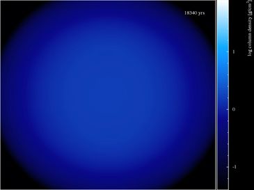
Initial Mass Function ( )
                                                M0 = Initial Mass                         S converted into stars

                                                Molecular Cloud

                                                                             S
                                                                   ⌘SF    =            (star formation efficiency)
                                                                            M0

-    We all learn in introductory astronomy classes that a star’s mass is the main characteristic that determines its evolution and eventual fate. Therefore,
     one of the first things that we should try to understand about a stellar population is the mass of the stars that comprise it.
-   The initial mass function (phi) is generally defined as the distribution of stars within a particular mass range that are formed when a net mass (delta S) is
    converted into new stars.
-   The efficiency of the star formation process (defined as the fraction of gas from a molecular cloud that is converted into stars) is also an important
    parameter that can be measured using mass functions. This is thought to be directly proportional to the difference between the IMF and CMF (more on
    this later).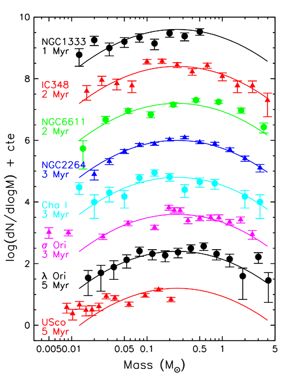
M (M ) ⌘
                                                              Z   Mmax
                                                                            (M )dM = 1
                                                                  Mmin

                                            (M )dM = number fraction of stars between M and M+dM
                                            (M )dM = mass fraction of stars between M and M+dM

-      With this simple cartoon model of star formation in place, the total number of stars between the masses M1 and M2 becomes the integral of the IMF
       between the masses M1 and M2.
-    Similarly, the total mass of all the stars between the the mass interval M1 to M2 can be found by integrating the IMF multiplied by the mass per star (M).
     This factor (M*phi) is sometimes defined as chi.
-    When comparing two stellar populations of different sizes, they may have a different number of stars in a given mass range simply because they have
     different total numbers of stars. However, they may have a similar fraction of stars within a particular mass range. For this reason, it is generally
     necessary to normalize phi and chi across the total star mass range so that they become indicators of the number and mass fraction of stars within a
     particular mass range.
Salpeter IMF is given by phi = K M^-2.35
    - This holds for stars with masses above ~ 1 M_sun
    - Normalizing phi and chi in this manner allow them to be interpreted as the number and mass fractions of stars between some mass range with respect
to the entire population.
    - Quick calculations show that the fraction of stars above one solar mass is about 5% while the total mass of stars greater than one solar mass is 40% of
the total mass of all the stars in the population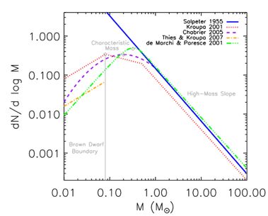
IMF Flavors

                                                  Offner et al. 2014

- Normalized so that the integral over mass is equal to one
Salpeter - 1955 fit available star data to a power law between 0.4 and 10 M_sun
Kroupa - later became apparent that the Salpeter IMF diverged at low masses. Series of piecewise power law functions across the lower masses began to
appear
Chabrier - log-normal up to a solar mass, then turns into a power law tail
*This is not an exhaustive list!!! Many other forms of the IMF have been created
Observations
of the IMF
Offner et al. 2014
- Figure shows recent IMF estimates for 8 young star forming regions. Error bars show root N error for each binned data point. Solid lines are NOT a fit
to the data but a scaled Chabrier IMF normalized to best follow the data. Regions must be young to get the best estimate of the initial mass function,
which can be significantly different from the present day mass function for clusters with older ages.
Three steps for determining IMF (this is difficult and contains many uncertainties):
1. Observe luminosity function (LF) for sample of stars that lie within some volume (generally observe either newly formed clusters, as shown in figure, or
field stars then try to extrapolate backwards using knowledge of stellar evolution. First method is difficult because these types of regions are still
usually enshrouded in dust which complicates the measurement of luminosity. The later method provides immense sample sizes but extrapolating back
is not a trivial problem.
2. Convert LF into Mass Function using mass-magnitude relation
3. Corrections applied for: star formation history and stellar evolution (young/old), binarity, etc.
- These IMFs show little variations from one another, all having characteristic peaks somewhere between 0.1 and 1 solar masses, which shows the
surprising universality of the IMF.Origins of the IMF
Nature vs. Nurture
• Stellar masses • Star formation is
inherited from natal fuelled by dynamical
core masses interactions
! !
• Predicting IMF • IMF can be
reduces to reproduced by
understanding the core competition between
mass function (CMF) accreting protostars
- The origins of the near universality of the IMF are still a debated problem within the star formation community. Generally, there are two sides of the
argument. On one hand, some believe the IMF is directly related to the CMF (core mass function) and that stars masses are set by the dense gas cores
from which they form. On the other hand, some believe that the IMF is independent of the CMF and that the observed mass spectrum can be
reproduced by the competition over the gas reservoirs within a molecular cloud by the forming population of protostars.
- Relic of the Core Mass Function? (which one can imagine is the analogue of the stellar IMF to dense core [the precursors of future stars])
-Core Mass Function
Kirk et al. 2013
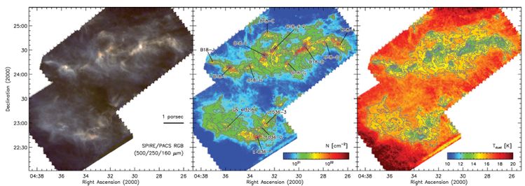
- Recent observations by the Herschel Space Observatory have shown that most stars form inside cold dense cores (r~0.1pc, densities ~ 10^5 cm^3,
T~10K) that lie within a larger web-like filamentary structure that permeates throughout molecular clouds. Material is thought to be carried to star
forming clusters inside the filaments by sub-filaments (aka striations), which are generally seen running perpendicular to the main filaments and have
also been found to follow the magnetic field lines of molecular clouds.
- Shown is a Herschel false color image and column density map for a region in the Taurus molecular cloud. Two distinct filaments can be seen running
east to westCore Identification
Kirk et al. 2013
- Dense cores are identified using source extraction algorithms that generally utilize the density contours from column density maps derived from sub
millimetre observations of a particular molecular cloud. Examples: clumpfind, CSAR, getsources, etc.
- There are many different source extraction routines and they all work somewhat differently (some use density contours some don’t, some take into
account the background level of the image while others don’t, some take into account multi-wavelength data at multiple spatial scales, while others
don’t .
- Best approach to take is to use two separate algorithms, one as a main method for source identification and one as a cross-check. All sources identified
by both algorithms are then classified as a core.
- Cartoon shown displays the differences in source sizes identified by two different algorithms. Four peaks A-D. Red shows the areas around each peak
that would be assigned to them by CSAR. The blue regions show the additional area that would be assigned to each peak using clumpfind.
- After these algorithms are run over a particular region, a source catalog is obtained. From this, the column densities within each source’s defined area
can be integrated to obtain the core’s mass, from which a CMF can be plotted.Pipe Nebula
CMF
⌘SF = 30% ± 10%
Alves et al. 2007
- CMF obtained from the Pipe Nebula. Black dots show the binned mass data. While the gray line shows the stellar IMF for the Trapezium cluster. Dashed
line shows the same IMF shifted by about a factor of 3, which indicates a uniform star formation efficiency around 30% will characterize the star formation
in this region.Origins of the CMF
Price et al. 2010
- This simulation of the collapse of a dense core and subsequent formation of a new protostar clearly display the culprit that is thought to cause the
IMF/CMF relationship. >>> Protostellar outflows
- The origin of the IMF/CMF relationship and the derived star formation efficiency is thought to be a direct byproduct of the protostellar outflows
generated after the birth of a newly formed star. These outflows could be disruptive enough to limit the accretion of mass onto a forming protostar,
limiting its final mass. Theoretical works have shown that outflows can produce star formation efficiencies around 30%, which match observational star
formation efficiencies derived from CMFsAlves et al.
2007
Kirk et al. 2013
1. Source extraction algorithms are far from perfect because there is no strict definition for a dense core. (See examples shown) CSAR identified cores
- which contour outlines the true core? Pick a contour and integrate the mass inside to determine the core mass.
2. Not all dense cores go on to form stars. May be identifying some low-mass cores that are “transient fluff” and will not form stars in the future.
- Take away message: don’t be naive when it comes to the CMF. Understand the uncertainties that go into the identification of cores and the difficulties
that arise when attempting to place a core within a finite size.You can also read