Imitation Learning via Reinforcement Learning of Fish Behaviour with Neural Networks
←
→
Page content transcription
If your browser does not render page correctly, please read the page content below
Freie Universität Berlin
  Bachelor’s Thesis at the Department for Informatics and Mathematics
  Dahlem Center for Machine Learning and Robotics - Biorobotics Lab

 Imitation Learning via Reinforcement
Learning of Fish Behaviour with Neural
               Networks

                                Marc Gröling
                        Matriculation Number: 5198060
                          marc.groeling@gmail.com

                   Supervisor:       Prof. Dr. Tim Landgraf
               First Examiner:       Prof. Dr. Tim Landgraf
             Second Examiner:        Prof. Dr. Dr. (h.c.) Raúl Rojas

                              Berlin, April 26, 2021

                                      Abstract
   The collective behaviour of groups of animals emerges from interaction be-
tween individuals. Understanding these interindividual rules has always been
a challenge, because the cognition of animals is not fully understood. Artificial
neural networks in conjunction with attribution methods and others can help
decipher these interindividual rules. In this thesis, an artificial neural network
was trained with a recently proposed learning algorithm called Soft Q Imitation
Learning (SQIL) on a dataset of two female guppies. The network is able to out-
perform a simple agent that uses the action of the most similar state in defined
metric and also is able to show most characteristics of fish, at least partially, when
simulated.
Eidesstattliche Erklärung
Ich versichere hiermit an Eides Statt, dass diese Arbeit von niemand anderem als
meiner Person verfasst worden ist. Alle verwendeten Hilfsmittel wie Berichte, Bücher,
Internetseiten oder ähnliches sind im Literaturverzeichnis angegeben, Zitate aus frem-
den Arbeiten sind als solche kenntlich gemacht. Die Arbeit wurde bisher in gleicher
oder ähnlicher Form keiner anderen Prüfungskommission vorgelegt und auch nicht
veröffentlicht.
April 26, 2021
Marc Gröling
34
Contents
1   Introduction                                                                                                                                   7

2   Theoretical Background                                                                                                                        8
    2.1 Reinforcement Learning . . . . . . . . . . . . . . . . . . . . . . . . . . . .                                                            8
    2.2 Q-learning and soft Q-learning . . . . . . . . . . . . . . . . . . . . . . . .                                                            8
    2.3 Soft Q Imitation Learning . . . . . . . . . . . . . . . . . . . . . . . . . . .                                                           8

3   Related Work                                                                                                                                   9

4   Implementation                                                                                                                                10
    4.1 Environment . . . . . . . . . . . . . . . . . .                       .   .   .   .   .   .   .   .   .   .   .   .   .   .   .   .   .   10
        4.1.1 Action Space . . . . . . . . . . . . .                          .   .   .   .   .   .   .   .   .   .   .   .   .   .   .   .   .   10
        4.1.2 Observation Space . . . . . . . . . .                           .   .   .   .   .   .   .   .   .   .   .   .   .   .   .   .   .   10
    4.2 Data . . . . . . . . . . . . . . . . . . . . . . .                    .   .   .   .   .   .   .   .   .   .   .   .   .   .   .   .   .   11
        4.2.1 Extraction of turn values from data                             .   .   .   .   .   .   .   .   .   .   .   .   .   .   .   .   .   11
    4.3 Model . . . . . . . . . . . . . . . . . . . . . .                     .   .   .   .   .   .   .   .   .   .   .   .   .   .   .   .   .   12
    4.4 Training . . . . . . . . . . . . . . . . . . . .                      .   .   .   .   .   .   .   .   .   .   .   .   .   .   .   .   .   13

5   Evaluating the Model                                                                                                                          14
    5.1 Metrics . . . . . . . . . . . .   .   .   .   .   .   .   .   .   .   .   .   .   .   .   .   .   .   .   .   .   .   .   .   .   .   .   14
         5.1.1 Rollout . . . . . . . .    .   .   .   .   .   .   .   .   .   .   .   .   .   .   .   .   .   .   .   .   .   .   .   .   .   .   14
         5.1.2 Simulation . . . . . .     .   .   .   .   .   .   .   .   .   .   .   .   .   .   .   .   .   .   .   .   .   .   .   .   .   .   16
    5.2 Choice of Hyperparameters         .   .   .   .   .   .   .   .   .   .   .   .   .   .   .   .   .   .   .   .   .   .   .   .   .   .   16
    5.3 Results . . . . . . . . . . . .   .   .   .   .   .   .   .   .   .   .   .   .   .   .   .   .   .   .   .   .   .   .   .   .   .   .   17

6   Discussion and Outlook                                                                                                                        24
    6.1 Cognition of the Model . . . . . . .              .   .   .   .   .   .   .   .   .   .   .   .   .   .   .   .   .   .   .   .   .   .   24
    6.2 Consider Observations of the Past                 .   .   .   .   .   .   .   .   .   .   .   .   .   .   .   .   .   .   .   .   .   .   24
    6.3 Different Learning Algorithms . .                 .   .   .   .   .   .   .   .   .   .   .   .   .   .   .   .   .   .   .   .   .   .   24
    6.4 Hyperparameter Optimization . .                   .   .   .   .   .   .   .   .   .   .   .   .   .   .   .   .   .   .   .   .   .   .   24

List of Figures                                                                                                                                   25

Bibliography                                                                                                                                      25

A Appendix                                                                                                                                        27
  A.1 Additional figures from simulated tracks . . . . . . . . . . . . . . . . . .                                                                27
  A.2 General insights about SQIL . . . . . . . . . . . . . . . . . . . . . . . . . .                                                             29
  A.3 Data and source code . . . . . . . . . . . . . . . . . . . . . . . . . . . . . .                                                            29

                                                      5
6
1. Introduction

1   Introduction
Almost every animal shows some form of collective behaviour in its life [9]. For some
animals this can be extremely well-coordinated, making the group seem like a single
unit. The comprehension of these inter-individual rules of a species could lead to a
better understanding of the behaviour of that species in general, as well as to a better
understading of the behaviour of other kinds of animals. The question, how the col-
lective behaviour of a species emerges from the interactions of individuals and how
these interaction rules work has attracted many scientists in the past and has resulted
in researchers creating minimalistic models (see [7], [5]) of fish. While these minimal-
istic models have been successful in approximating collective behaviour (see [15]), it is
very difficult to create accurate interaction rules without fully understanding animal
cognition [8].
     As a result of this lack of knowledge, another more novel method becomes more
attractive: modelling the behaviour of fish or animals in general with an artificial
neural network. This way interaction rules do not have to be defined in advance but
rather can be derived later from the learned network with attribution methods for
example. Besides, these models can be used to control robotic fish and replace living
social interaction partners. This "can help elucidate the underlying interaction rules
in animal groups." [10].
     The even further increase in computational power and the creation of new meth-
ods and improvement of old ones in AI research has made the approach of modelling
animal behaviour with an artificial neural network even more appealing. In this the-
sis, a recently proposed learning method called Soft Q Imitation Learning (SQIL) was
used to model fish behaviour, specifically guppies.

In section 2 the theoretical background of the learning method is set, which is followed
by section 3, where similiar work is reviewed and it is clarified how this thesis differs
from them. Later on in section 4 information about how the agent perceives the world
and interacts with it is presented, as well as information about the data that was used
to train the model and facts about the model itself and the training process. In the
following section, section 5 the metrics to quantify the behaviour of the model are
defined, as well as the choice of hyperparameters and the results of the obtained
model are shown. Finally, section 6 provides a summary of the completed work as
well as providing information about possible improvements and further experiments
that could lead to additional insights.

                                           7
2. Theoretical Background
2 Theoretical Background
2.1 Reinforcement Learning
Humans and other beings learn by interacting with their environment, they learn
about the causes and effects of their actions and what to do in order to achieve goals.
Reinforcement learning uses this idea by exploring an environment and learning how
to map situations to actions in order to maximize a numerical reward signal. Actions
might not only affect immediate reward but also subsequent rewards. "These two
characteristics - trial-and-error search and delayed reward are the two most important
distinguishing features of reinforcement learning." [13]
2.2 Q-learning and soft Q-learning
"Q-learning provides a simple way for agents to learn how to act optimally in Marko-
vian domains." [3] It uses a Q-function that gives an estimate of the expected reward
of an action. This function considers short-term and long-term rewards, by apply-
ing a discount factor on rewards that are further away in time. The accuracy of the
Q-function is continuously improved by collecting transitions in its environment and
updating the Q-function accordingly. "By trying all actions in all states repeatedly, it
learns which are the best overall." [3]
The difference between Q-learning and soft Q-learning is that soft Q-learning also
considers the entropy of a policy, which is a measure of randomness. This change
makes the policy learn all of the ways of performing a task instead of only learning
the best way of performing it. [4]
2.3 Soft Q Imitation Learning
Soft Q Imitation Learning (SQIL) performs soft Q-learning with three modifications:
(1) it stores all expert samples into an expert replay buffer with a constant reward
set to one; (2) it collects exploration samples in the environment and stores them in
an exploration replay buffer with a constant reward set to zero; (3) when training it
balances samples from the expert replay buffer and the exploration replay buffer (50%
each). [12]
As a result of these modifications, the agent is encouraged to imitate demon-
strated actions in demonstrated states and to return to demonstrated states, when
it encounters non-demonstrated states [12]. Therefore it is able to overcome the is-
sue of tending to drift away from demonstrated states, which is common in standard
behavioural cloning that uses supervised learning. [14]
83. Related Work
3 Related Work
There have already been several approaches to model animal behaviour, specifically
fish behaviour:
In [6] the authors used inverse reinforcement learning to predict animal movement in
order to fill in missing gaps in trajectories. However their work was done on a larger
scale and opposed to this work an explicit reward function had to be defined.
In [7] the authors created a minimalistic model of handcrafted rules that was success-
ful in approximating characteristics of swarm behaviour of fish. This model works
with zones of attraction, orientation and repulsion that would determine the be-
haviour of an individual.
In [11] the author successfully trained recurrent neural networks to predict fish loco-
motion. Their model uses observations of the past, opposed to the one presented in
this thesis, as well as it being trained with behavioural cloning. This publication was
a huge inspiration for this thesis and as a result, most of their design choices were
adopted.
In [2] the authors used quality diversity algorithms, which emphasise exploration
over optimisation, in conjunction with feedforward neural networks to train models
to predict zebrafish locomotion. Their model uses a different kind of input, which
gives direct information of the previous locomotion and distances and angles towards
other agents, as well as the nearest wall.
In [8] the authors successfully trained a feedforward network with behavioural cloning
on lampeye fish data. Their input consists of the fishes own velocity, the sorted posi-
tion and velocity of the three nearest neighbours, as well as the distance and angle of
the nearest wall.
94. Implementation
4 Implementation
4.1 Environment
RoboFish is a project of the Biorobotics Lab that uses a robotic fish that is placed into
an obstacle-free 100 cm x 100 cm tank. For experiments live fish can be added to the
tank. The robotic fish can be controlled via Wi-Fi, a magnet underneath the tank and
corresponding soft- and hardware.
Additionally, there exists an associated OpenAi gym environment that mimics the
RoboFish environment: Gym-Guppy1 . While this environment can be configured in
many ways, only the settings used for thesis are mentioned in the following. All
training and testing of agents was done in this environment.
The environment consists of a 100 cm x 100 cm tank in which fish (agents) can
be added and then simulated at a frequency of 25 Hz. At each timestep, the agent
has to provide a turn and speed value, which will move it accordingly until the next
timestep. An agent has the following poses: x-position, y-position and orientation
in radians. At the edges of the tank, there are walls that stop any fish from straying
outside of the tank.
4.1.1 Action Space
The action space of an agent consists of the following pair:
• The angular turn in radians for the change in orientation from timestep t-1 to t.
• The distance travelled from timestep t-1 to t.
These actions are then executed as follows: First, the agent turns by the angular
turn value and then performs a forward boost, moving it by the predicted distance.
As a result of the two-dimensional action space, the agents cannot represent lat-
eral movement. This should not be an issue though, since the same data was used
in [11] and the author "did not observe any guppy actually performing such lateral
movement". Additionally adding another orientation action would result in higher
complexity, while probably adding only little information, which is why it is not in-
cluded.
4.1.2 Observation Space
The observations of the agent are very similar to a minimalistic virtual eye: Raycasts.
This kind of observation was also used in [11]. These raycasts are split into two
categories:
• View of walls: This is done by casting a fixed number of rays in the field of
view (fov) centered around the fish and measuring the distance between the
fish and each wall. These distances [0, far_plane] (far_plane being the length of
the diagonal of the tank) are then linearly scaled into intensity values [1, 0]. An
1 https://git.imp.fu-berlin.de/bioroboticslab/robofish/gym-guppy
104.2 Data
intensity value close to to one tells the agent that the wall is nearby and close to
zero that it is far away. An example of this is displayed in Figure 1.
• View of other agents: This is done by again casting rays in the field of view, but
now searching for other agents in the sectors that are between these rays and
measuring the distance to them. The distance to the closest agent in each sector
is then normalized into [1, 0] intensity values, like in raycasting of walls. This
can be seen in Figure 1, with shades representing the intensity value (black = 1,
white = 0).
(a) View of walls raycasting: 180° fov, 5 (b) View of agents raycasting: 180° fov, 4
rays [11] sectors [11]
Figure 1: Raycasting of walls and agents
4.2 Data
The data used for training is the same as the live data in [11]. In short, these trajec-
tories were created by placing 2 female guppies into a for them unknown 100 x 100
cm tank. Video footage of them swimming in the tank was then captured for at least
10 minutes at a frequency of 25 Hz. For pose extraction, the idtracker.ai software was
used in order to extract x,y and orientation values. Data was also cleaned and cut.
Further information on the creation and processing of these trajectories can be read
in [11].
4.2.1 Extraction of turn values from data
As mentioned in subsubsection 4.1.1 models move by first turning into the desired
direction and then moving along that direction according to a speed value. As a result,
if a fish in training data would turn into a direction then perform a forward boost
and then turn again, the last orientation change could not be represented directly by
defined action space. Therefore turn values were extracted the following way:
Let v1 be the vector that points from the position at timestep t-1 to the position at
timestep t and let v2 be the vector that points from the position at timestep t to the
114. Implementation
position at timestep t+1. Let the turn value be the angle α ∈ [0, 2π ) between v1 and
v2 . An example of this can be seen in Figure 2.
Figure 2: Extraction of turn value α at timestep t
4.3 Model
For this thesis, SQIL was used. In order to implement SQIL, the DQN implementation
from stable-baselines2 was used and adjusted such that the learning function would
work as described in subsection 2.3.
As Input the model receives a handcrafted feature vector, that consists of ray-
casts as mentioned in subsubsection 4.1.2. These raycasts are given only for the latest
timestep, also the model does not have an interior state. The model network is a
simple feedforward network. As a result, the model’s decisions are based entirely on
current observations, which assumes a Markov decision process, which might not be
given with the problem of modelling fish behaviour.
As Output the model had to predict a turn and a speed value that it would travel
for the next timestep (as mentioned in subsubsection 4.1.1). However since a DQN
was used and the stable-baselines implementation would only accept discrete action
spaces, the output was discretized by approximating turn/speed values with bins in
a linear range for each action component. At first, a matrix-oriented discretization
method (both actions are encoded in one number) was used, however this would re-
sult in an overflow of possible actions (number of possible turn values * number of
possible speed values). In order to have the necessary precision when predicting ac-
tions, two DQNs were used instead of one. Each DQN would then predict one of the
two action components respectively and as a result each model would have far fewer
possible actions to consider.
2 https://stable-baselines.readthedocs.io/en/master/modules/dqn.html
124.4 Training
4.4 Training
For training agents, the created SQIL implementation was used (see subsection 4.3).
Training was done using the Gym-Guppy environment by spawning two fish (agents)
that are controlled by the model into the tank and then having them collect exploration
data that is then stored in a replay buffer. Due to the fact that 2 neural networks were
used for predicting movement, they were trained sequentially. The main reason for
this decision were time constraints and ease of implementation. The networks would
collect samples by exploring 1000 timesteps at a time and then the other network
would take part in exploring. Explored samples are added to the replay buffer of
both DQNs. Whenever the exploring network was switched, the environment was
reset in order to avoid any problems such as agents continously swimming into walls.
When resetting the environment both agents would be spawned into a uniformly
random pose of the tank with the only restriction being that it is at least 20 cms away
from any wall.
135. Evaluating the Model
5 Evaluating the Model
5.1 Metrics
In order to evaluate models two types of metrics were used: Simulating the model in
a tank and evaluating its trajectory with different functions (Simulation), as well as
comparing predictions of actions of the trained model in validation data with actions
of live fish (Rollout).
5.1.1 Rollout
The guppies are not moving deterministically in the training data which makes eval-
uation of a models performance way harder, since one cannot assume that there exists
only one valid action for each observation. As a result when evaluating if an action
is correct for a given observation, one may consider other observations that are some-
how similar to the original observation and taking the actions of these "similar" states
into account. This can be applied to similar actions too.
In this section, these kinds of similarities were defined in order to get a meaning-
ful statement about the model’s ability to abstract from training data.
Definition of similarity of observations: Let two observations be "similar" if the dis-
tance between these two observations is smaller than threshold x.
Definition of the distance between observations: Let the distance between two ob-
servations o1 and o2 be the sum of the distances between single components of the
observation: distance between fish-raycasts and distance between wall-raycasts.
• Distance between wall-raycasts: Let the distance between wall-raycasts be:
numrays
∑ abs(o1 .wall_ray[i ] − o2 .wall_ray[i ])
i =1
• Distance between fish-raycasts: Since in all experiments there are only two fish
in the tank at a time, the distance between fish-raycasts can be defined as the
actual distance in centimetres between seen fish in raycasts of o1 and o2 . This
means that the relative fish position of o1 and o2 is reconstructed with infor-
mation from fish-raycasts with the original fish at the center of the coordinate
system. Then the distance between the fish seen in o1 and o2 is taken.
The significance of both components of the observation should be similar, because
otherwise one part might dominate artificially. As a result, they were scaled (as seen
in Figure 3) such that when taking the pairwise distance between all observations in
validation data the mean of fish-raycasts and wall-raycasts is the same.
145.1 Metrics
Figure 3: Pairwise distances of observations in validation data: Impact of different
distance components (after scaling)
Setting of threshold x: Threshold x is chosen by taking the pairwise distance between
all observations in validation data and then taking the y% smallest distance (e.g.: 1%
smallest, 2% smallest..). As a result on average, the y% closest observations are con-
sidered "similar".
To create a score the model is given the observation for all state-action pairs in val-
idation data. Then the model’s prediction is compared with the allowed actions for
this state, if it is accepted, then a reward of one is given else a reward of zero is given.
Allowed actions are actions that come from observations that are similar (as defined
above) to the original observation. Additionally, if an action is only a maximum of 1
mm away in speed value and 2 degrees in turn value from an action in allowed ac-
tions, then it is still accepted. Finally, the mean of all these rewards is taken, resulting
in a score between 0 and 1 that measures how well the agent learned from training
data and is able to abstract to non-seen validation data.
To have a better idea of the model’s performance, additional agents were added
to the comparison: an agent that takes random actions, a perfect agent and finally
the closestStateAgent that would always perform the action of the state with minimal
distance to the original observation in training data.
155. Evaluating the Model
Additionally, these scores were separately computed where the distance function
only considers either fish-raycasts or wall-raycasts for determining the distance be-
tween two observations.
5.1.2 Simulation
In simulation two fish, that are being controlled by the model, are spawned into the
tank with a uniformly random pose that is at least 5 cms away from any wall. Both
agents would then move for 10000 timesteps according to model predictions, resulting
in footage of 6 minutes and 40 seconds at a frequency of 25 Hz. To avoid recurring
trajectories, the model’s predictions are not deterministic for this experiment, but have
a heavy favor towards these actions.
To quantify fish behaviour of these trajectories the following metrics that were also
used in [11] were used: linear speed, angular speed, interindividual distance, follow,
tank position heatmaps and trajectory plots.
Additionally, the following metrics were designed to help evaluate models in this
thesis: relative orientation (between agents), distance to the nearest wall, orientation
heatmaps of the tank, relative position of the other agents to one’s own as a heatmap.
5.2 Choice of Hyperparameters
Parameter Value range
Number of hidden layers 1-4
Number of neurons per hidden layer 16 - 512
Layer normalization on, off
Explore fraction 0.01 - 0.5
Gamma 0.5 - 0.999
Learnrate 1e-6 - 1e-3
Batchsize 1 - 128
Learn timesteps 5000 - 3e5
Clipping during training on, off
Table 1: Ranges for hyperparameters
For the setting of hyperparameters, a hyperparameter optimization framework called
Optuna [1] was used with the following ranges for hyperparameters, as shown in
Table 1. The objective function to maximize is the average reward of the last 5 Rollout
samples, with the distance function considering both fish- and wall-raycasts and a
threshold x of 7.17 (1% closest observations). To make optimization easier the same
model hyperparameters were used for both DQNs.
An explanation of each model hyperparameter can be found in the stable-baselines
documentation for DQN’s3 except for clipping during training, which as the name
suggests makes sure that no action would lead to a collision between agent and walls
3 https://stable-baselines.readthedocs.io/en/master/modules/dqn.html
165.3 Results
of the tank. Additionally, since SQIL always trains with a 50/50 ratio between expert
and exploration samples, batchsize is the number of samples that are extracted each
time the weights of the neural network are updated.
5.3 Results
With Optuna 32 trials were run, in which hyperparameters were suggested, a model
was trained and then evaluated. A representative network was then chosen, by con-
sidering both how realistic the observed behaviour of the fish was when simulated
and how good the achieved score of the model was. Hyperparameters of this model
are shown in Table 2.
Parameter Value
View of agents 360° fov, 36 sectors
View of walls 360° fov, 36 rays
Linear speed 0 - 2 cm/timestep, 201 bins
Angular speed -pi - pi radians/timestep, 721 bins
Hidden layer 0 # neurons 81
Hidden layer 1 # neurons 16
Layer normalization off
Explore fraction 0.483
Gamma 0.95
Learnrate 4.318e-5
Batchsize 2
Learn timesteps 163000
Clipping during training off
Table 2: Hyperparameters of the representative network
Rollout scores during the training process of the representative network can be
seen in Figure 4, 5 and 6. The difference between these three figures is the way how
the distance function is computed (can be seen in the caption of the corresponding
figure). The score of the model increases swiftly and after about 10000 timesteps of
training, the model already outperforms the closestStateAgent in all three variations
of Rollout. Then the score almost stagnates after about 20000 timesteps of training.
The score of the model and the closestStateAgent is in Figure 6 especially high, which
suggests that the interaction with walls is rather easy in comparison to the interaction
with other fish and the combining of the two. Furthermore, the distances of 1% and
2% closest states in Figure 4 is almost double the magnitude of the corresponding
distances of the single components. This might be an indicator that not enough train-
ing data was used. Finally, the model outperforms the closestStateAgent in all three
Rollout metrics by at least 0.08, which hints that the model has learned to abstract
from training data to non-seen validation data.
175. Evaluating the Model
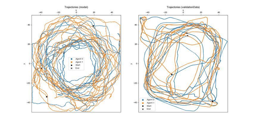
Figure 7, 8, 9, 10, 11 and 12 show the behaviour of the model in simulated tracks.
When considering Figure 7 and 8 it becomes apparent that the model has learned that
the fish generally avoid the center of the tank, however, it seems that the model has
not fully learned the positional preference of the fish that is close to the walls of the
tank. Moreover, while the model is able to approximate the behaviour of the fish with
regards to the follow metric, seen in Figure 9, it has not learned that the fish swim in
close proximity to each other (< 20cm) for most of the time. In Figure 10 one can see
that the model has a very similar distribution of speed values as the fish in validation
data and it also was able to adapt the behaviour of the fish swimming around the
tank clockwise, as seen in Figure 11. Finally, Figure 12 shows that the model has a
greater favour for turning right rather than left, which cannot be said about the fish
in validation data, which seem to not prefer either.
Figure 4: Rollout values during the training process of the model (distance function
considers both fish- and wall-raycasts)
185.3 Results
Figure 5: Rollout values during the training process of the model (distance function
considers only fish-raycasts)
195. Evaluating the Model
Figure 6: Rollout values during the training process of the model (distance function
considers only wall-raycasts)
205.3 Results
Figure 7: Trajectories: model (left) and valdation data (right, only one file)
Figure 8: Distance to closest wall distribution: model (left) and validation data (right)
215. Evaluating the Model
Figure 9: Follow/iid: model (left) and validation data (right)
Figure 10: Speed distribution: model (left) and validation data (right)
225.3 Results
Figure 11: Mean orientations in radians: model (left) and validation data (right)
Figure 12: Turn distribution in radians: model (left) and validation data (right)
236. Discussion and Outlook
6 Discussion and Outlook
In this thesis, a model was trained with SQIL on trajectories of guppies that was able
to show some characteristics of fish behaviour. The model is generally able to outper-
form an agent that considers the action of the most similar state of training data in
defined metric, as well as being able to show most of the characteristics of fish when
creating a simulated track, at least partially.
Now further research can be done with the obtained model in order to help un-
derstand interindividual interaction in guppies, which might be applicable to other
species as well. This could be done by using attribution methods or having the model
interact with live fish for example. Unfortunately, this was not feasible within the
scope of this thesis.
Since the model was not able to fully imitate fish behaviour, refinement of it would
be advantageous. Improvements could be, but are not limited to the following:
6.1 Cognition of the Model
As already mentioned in section 1 the cognition of fishes is not fully understood and
thus the raycasts-based observations might not be as good of a way to model the
environment of an agent. One could add additional information about the environ-
ment such as the orientation of other agents or try a completely different approach of
modelling the environment of an agent.
6.2 Consider Observations of the Past
The model trained in this thesis does not receive any information about its environ-
ment apart from the raycasts of the current timestep. It would be interesting to see
whether and how the model’s performance would change if one would use a recur-
rent neural network instead of using a feedforward network or to use a feedforward
network but feed informations about the last few timesteps into it.
6.3 Different Learning Algorithms
The reward structure that was used in SQIL could also be applied to an Actor Critic
method or in general an algorithm that learns a policy immediately instead of learning
a Q-function and then deriving a policy from it. This might benefit the performance
of the model and thus it would be interesting to try.
6.4 Hyperparameter Optimization
The current function to maximize in hyperparameter optimization only considers the
ability to reproduce actions in validation data. However this does not imply that the
model’s trajectories when simulated are considering all aspects seen in data. Another
aspect of SQIL is that it is supposedly able to return to demonstrated states when
it encounters out-of distribution states. It would be interesting to see how well the
current model performs if one defines a function that also considers these aspects, as
well as how the hyperparameters change with a new objective to maximize.
24List of Figures
List of Figures
1 Raycasting of walls and agents . . . . . . . . . . . . . . . . . . . . . . . . 11
2 Extraction of turn value α at timestep t . . . . . . . . . . . . . . . . . . . 12
3 Pairwise distances of observations in validation data: Impact of differ-
ent distance components (after scaling) . . . . . . . . . . . . . . . . . . . 15
4 Rollout values during the training process of the model (distance func-
tion considers both fish- and wall-raycasts) . . . . . . . . . . . . . . . . . 18
5 Rollout values during the training process of the model (distance func-
tion considers only fish-raycasts) . . . . . . . . . . . . . . . . . . . . . . . 19
6 Rollout values during the training process of the model (distance func-
tion considers only wall-raycasts) . . . . . . . . . . . . . . . . . . . . . . . 20
7 Trajectories: model (left) and valdation data (right, only one file) . . . . 21
8 Distance to closest wall distribution: model (left) and validation data
(right) . . . . . . . . . . . . . . . . . . . . . . . . . . . . . . . . . . . . . . . 21
9 Follow/iid: model (left) and validation data (right) . . . . . . . . . . . . 22
10 Speed distribution: model (left) and validation data (right) . . . . . . . . 22
11 Mean orientations in radians: model (left) and validation data (right) . 23
12 Turn distribution in radians: model (left) and validation data (right) . . 23
13 Relative orientation of agents: model (left) and validation data (right) . 27
14 Tank positions: model (left) and validation data (right) . . . . . . . . . . 28
15 Vector to other fish: model (left) and validation data (right) . . . . . . . 28
Bibliography
[1] Takuya Akiba, Shotaro Sano, Toshihiko Yanase, Takeru Ohta, and Masanori
Koyama. Optuna: A next-generation hyperparameter optimization framework.
In Proceedings of the 25rd ACM SIGKDD International Conference on Knowledge Dis-
covery and Data Mining, 2019.
[2] Leo Cazenille, Nicolas Bredeche, and José Halloy. Automatic calibration of arti-
ficial neural networks for zebrafish collective behaviours using a quality diver-
sity algorithm. In Uriel Martinez-Hernandez, Vasiliki Vouloutsi, Anna Mura,
Michael Mangan, Minoru Asada, Tony J. Prescott, and Paul F.M.J. Verschure,
editors, Biomimetic and Biohybrid Systems, pages 38–50, Cham, 2019. Springer In-
ternational Publishing.
[3] Peter Dayan Christopher J.C.H. Watkins. Q-learning. Machine Learning, 8, 279-
292, 1992.
[4] Tuomas Haarnoja, Haoran Tang, Pieter Abbeel, and Sergey Levine. Reinforce-
ment learning with deep energy-based policies. CoRR, abs/1702.08165, 2017.
[5] James E. Herbert-Read, Andrea Perna, Richard P. Mann, Timothy M. Schaerf,
David J. T. Sumpter, and Ashley J. W. Ward. Inferring the rules of interaction of
shoaling fish. Proceedings of the National Academy of Sciences, 108(46):18726–18731,
2011.
25Bibliography
[6] Tsubasa Hirakawa, Takayoshi Yamashita, Toru Tamaki, Hironobu Fujiyoshi, Yuta
Umezu, Ichiro Takeuchi, Sakiko Matsumoto, and Ken Yoda. Can ai predict an-
imal movements? filling gaps in animal trajectories using inverse reinforcement
learning. Ecosphere, 9:e02447, 10 2018.
[7] Richard James Iain D. Couzin, Jens Krause, Graeme D. Ruxton, and Nigel R.
Franks. Collective memory and spatial sorting in animal groups. Journal of
Theoretical Biology, 2002.
[8] Hiroyuki Iizuka, Yosuke Nakamoto, and Masahito Yamamoto. Learning of indi-
vidual sensorimotor mapping to form swarm behavior from real fish data. pages
179–185, 01 2018.
[9] Graeme D. Ruxton Jens Krause. Living in Groups. Oxford University Press, 2002.
[10] Tim Landgraf, Gregor H.W. Gebhardt, David Bierbach, Pawel Romanczuk, Lea
Musiolek, Verena V. Hafner, and Jens Krause. Animal-in-the-loop: Using interac-
tive robotic conspecifics to study social behavior in animal groups. Annual Review
of Control, Robotics, and Autonomous Systems, 4(1):null, 2021.
[11] Moritz Maxeiner. Imitation learning of fish and swarm behavior with Recurrent
Neural Networks. Master’s thesis, Freie Universität Berlin, 2019.
[12] Siddharth Reddy, Anca D. Dragan, and Sergey Levine. Sqil: Imitation learning
via reinforcement learning with sparse rewards, 2019.
[13] Andrew G. Barto Richard S. Sutton. Reinforcement Learning: An introduction. MIT
Press, 2018.
[14] Drew Bagnell Stéphane Ross, Geoffrey Gordon. A reduction of imitation learn-
ing and structured prediction to no-regret online learning. pages 627–635. In
Proceedings of the fourteenth international conference on artifical intelligence
and statistics, 2011.
[15] Iain D. Couzin Ugo Lopez, Jacques Gautrais and Guy Theraulaz. From be-
havioural analyses to models of collective motion in fish schools. 2012.
26A. Appendix
A Appendix
A.1 Additional figures from simulated tracks
Figure 13 shows the distribution of angles α ∈ [0, π ] between the orientation vectors
of the two fish. While the live fish have a slight preference for being either aligned or
orthogonal to each other, the model does not show this kind of behaviour and even
seems to prefer a 45° angle. In Figure 14 the tank positions of fish are displayed as a
heatmap, which shows similar properties of the model, such as Figure 7: The model
avoids the center of the tank like the live fish, but fails to fully learn the positional
preference of the live fish, which is close to the walls of the tank. Additionally, the
model completely avoids the corners of the tank, unlike the fish in validation data.
Last but not least, Figure 15 shows the relative position of the other fish to the original
one as a heatmap (rotated to match the original fish’s orientation). The model does
not show a certain preference in this figure, apart from what can already be seen in
Figure 9, which also shows the difference of interindividual distances between the
fish.
Figure 13: Relative orientation of agents: model (left) and validation data (right)
27A. Appendix
Figure 14: Tank positions: model (left) and validation data (right)
Figure 15: Vector to other fish: model (left) and validation data (right)
28A.2 General insights about SQIL
A.2 General insights about SQIL
While working with SQIL and in order to see if it would work on an easier problem
(and also to check if the SQIL implementation was working), I designed a modified
version of Cartpole4 . In this version contrary to the popular form, the pole would
start facing downwards rather than upwards. As a result, the model would have to
get the pole facing upwards first, by swinging it left and right repeatedly and then
balancing it.
The problem with this kind of task and SQIL is, that SQIL gets the same reward for
any action that can be found in the expert data set. The issue here is that the steps
to get the pole facing upwards are not the desired behaviour, but just the necessary
steps to get to the point where the algorithm can execute the desired behaviour. As a
result, the model may only partially understand the goal.
While training different models with SQIL for Cartpole I did not come up with a
truly good model that mastered the given task. The reason for this is probably (at
least partially) the problem explained above.
A.3 Data and source code
The data and source code is available in the corresponding GitHub repository:
https://github.com/marc131183/BachelorThesis
4 https://github.com/marc131183/gym-Cartpole
29You can also read