Impact of assimilating sea ice concentration, sea ice thickness and snow depth in a coupled ocean-sea ice modelling system - The Cryosphere
←
→
Page content transcription
If your browser does not render page correctly, please read the page content below
The Cryosphere, 13, 491–509, 2019
https://doi.org/10.5194/tc-13-491-2019
© Author(s) 2019. This work is distributed under
the Creative Commons Attribution 4.0 License.

Impact of assimilating sea ice concentration, sea ice thickness and
snow depth in a coupled ocean–sea ice modelling system
Sindre Fritzner1 , Rune Graversen1 , Kai H. Christensen2 , Philip Rostosky3 , and Keguang Wang4
1 UiT  The Arctic University of Norway, Tromsø, Norway
2 The  Norwegian Meteorological Institute, Oslo, Norway
3 Institute of Environmental Physics, University of Bremen, Bremen, Germany
4 The Norwegian Meteorological Institute, Tromsø, Norway

Correspondence: Sindre Fritzner (sindre.m.fritzner@uit.no)

Received: 20 August 2018 – Discussion started: 10 October 2018
Revised: 18 December 2018 – Accepted: 21 January 2019 – Published: 8 February 2019

Abstract. The accuracy of the initial state is very important      the seasonal forecast showed that assimilating snow depth
for the quality of a forecast, and data assimilation is crucial    led to a less accurate long-term estimation of sea-ice extent
for obtaining the best-possible initial state. For many years,     compared to the other assimilation systems. The other three
sea-ice concentration was the only parameter used for assim-       gave similar results. The improvements due to assimilation
ilation into numerical sea-ice models. Sea-ice concentration       were found to last for at least 3–4 months, but possibly even
can easily be observed by satellites, and satellite observations   longer.
provide a full Arctic coverage. During the last decade, an
increasing number of sea-ice related variables have become
available, which include sea-ice thickness and snow depth,
                                                                   1   Introduction
which are both important parameters in the numerical sea-ice
models. In the present study, a coupled ocean–sea-ice model        Observations show that for the last 50 years there has been a
is used to assess the assimilation impact of sea-ice thickness     decline in both Arctic sea-ice extent (Stroeve et al., 2007;
and snow depth on the model. The model system with the             Perovich et al., 2017) and sea-ice thickness (Kwok and
assimilation of these parameters is verified by comparison         Rothrock, 2009). In addition, models show that the sea-ice
with a system assimilating only ice concentration and a sys-       decline is likely to continue (Zhang and Walsh, 2006). Wang
tem having no assimilation. The observations assimilated are       and Overland (2012) estimate the Arctic Ocean to be nearly
sea ice concentration from the Ocean and Sea Ice Satellite         ice-free within the 2030s. This large change in the global cli-
Application Facility, thin sea ice from the European Space         mate system leads to a need for improved models and fore-
Agency’s (ESA) Soil Moisture and Ocean Salinity mission,           casting systems due to more variable and mobile Arctic sea
thick sea ice from ESA’s CryoSat-2 satellite, and a new snow-      ice (Eicken, 2013). In addition, a decreased amount of sea ice
depth product derived from the National Space Agency’s Ad-         will lead to increased Arctic ship traffic (Smith and Stephen-
vanced Microwave Scanning Radiometer (AMSR-E/AMSR-                 son, 2013). Safe travel in the Arctic is dependent on accu-
2) satellites. The model results are verified by comparing as-     rate knowledge of weather and sea ice. The Arctic is char-
similated observations and independent observations of ice         acterised by harsh conditions involving, for instance, sea ice,
concentration from AMSR-E/AMSR-2, and ice thickness                icebergs, and polar low storms. The numerical weather pre-
and snow depth from the IceBridge campaign. It is found            diction models are becoming more complex and detailed, but
that the assimilation of ice thickness strongly improves ice       still, the vital part of an accurate forecast is the model initial
concentration, ice thickness and snow depth, while the snow        state. Accurate initial states can be achieved by assimilating
observations have a smaller but still positive short-term ef-      observations into the model system.
fect on snow depth and sea-ice concentration. In our study,

Published by Copernicus Publications on behalf of the European Geosciences Union.
492                                                                       S. Fritzner et al.: The Metroms assimilation system

   For sea-ice modelling in the Arctic, observations are            The SMOS mission uses L-band passive microwave mea-
sparse. The sea-ice concentration (SIC), defined as the frac-       surements utilising long penetration depth and a relationship
tion of the total area covered by sea ice, has been available       between observed brightness temperature and ice thickness
since the start of the satellite era in 1979, but observations of   (Tian-Kunze et al., 2016). However, in general, the uncer-
other parameters such as sea ice thickness (SIT) are more dif-      tainties of the CryoSat-2 and SMOS SIT observations are
ficult to obtain because of the remote location, and satellites     high (Zygmuntowska et al., 2014; Xie et al., 2016), which
cannot easily be used to extract information about the SIT.         result in reduced, though still valuable, observational infor-
The passive microwave satellites derive SIC from bright-            mation available for assimilation into the model system. The
ness temperatures, but many of the Earth observing satellites       SIT observations are limited to winter conditions, when the
do not have sufficient wavelength to observe changes in the         snow and ice are dry.
brightness temperature as a function of the SIT. Thus, ac-             One of the first studies with SIT assimilation was done by
quiring SIT from satellites is significantly more difficult than    Lisæter et al. (2007). In this study, computer-generated SIT
acquiring SIC, but as will be described later, satellites using     observations simulating CryoSat observations were assimi-
the L-band frequency can, to some degree, be used to mea-           lated into a coupled ice–ocean model using the EnKF. The as-
sure the SIT as a function of brightness temperature.               similation showed significant effects on the model state; both
   During the last 15 years, there have been various studies of     improvements to the modelled SIT and multivariate effects
SIC assimilation using several different models and assimila-       on SIC, ocean temperature and ocean salinity were found.
tion methods. Lisæter et al. (2003) assimilated SIC obtained        Yang et al. (2014) used the localised singular evolutive inter-
from passive microwave satellite into a coupled ocean–ice           polated Kalman filter (Pham, 2001) to assimilate the SMOS
model using the ensemble Kalman filter (EnKF; Evensen,              SIT observations into the Massachusetts Institute of Tech-
1994; Burgers et al., 1998). In the study of Lisæter et al.         nology general circulation model (Marshall et al., 1997). In
(2003), the assimilation was found to have a strong effect          this study, an improved thickness forecast was found when
on the modelled SIC and small effects on other model pa-            assimilating SMOS observations and some improvements to
rameters due to the multivariate properties of the EnKF. The        the SIC forecasts. Similarly to Yang et al. (2014), Xie et al.
multivariate properties of the EnKF consist of a model up-          (2016) used the EnKF to assimilate SMOS SIT observations
date for all model variables based on correlation with the          into the TOPAZ system (Sakov et al., 2012). In this study it
observed variables. A similar SIC assimilation study using          was found that assimilation of SMOS observations showed
the 3D variational (3D-Var) assimilation method was done            improvements for the ice thickness along the ice edge, both
by Caya et al. (2010). In this study, both ice charts from the      compared to SIT observations not assimilated and compared
Canadian east coast and Radarsat 2 SIC observations were            to the SMOS observations themselves. In general, similarly
assimilated. Significant improvements to the short-term fore-       to that found by Yang et al. (2014) the SMOS observations
cast were found for the assimilation system. Studies with the       were found to have a relatively small impact on the SIC and
coupled ocean–ice model TOPAZ (Sakov et al., 2012) have             the SIT far from the ice edge. Fritzner et al. (2018) assim-
shown improvements to SIT and multivariate effects on SIT           ilated SMOS observations into a stand-alone sea-ice model
for assimilation of SIC (Sakov et al., 2012). Other SIC stud-       with the EnKF. This study showed that, due to the corre-
ies have been done by Lindsay and Zhang (2006) and Wang             lation between SIC and SIT, the SMOS observations were
et al. (2013), both using nudging methods to show model im-         found to have a positive effect on the modelled SIC. In the
provements for SIC assimilation. Posey et al. (2015) assimi-        last couple of years, there has also been an increase in the
lated high-resolution SIC observations (4 km) into a coupled        use of Cryosat-2 observations in various forms for assimila-
ocean–sea-ice model, the Arctic Cap Nowcast/Forecast Sys-           tion. Chen et al. (2017) assimilated both the SMOS thin SIT
tem (ACNFS) using the 3DVAR assimilation method. In this            and the CryoSat-2 thick SIT into the National Centers for En-
study, they showed that increased observation resolution has        vironmental Prediction’s (NCEP) Climate Forecast System
a significant impact on the ice edge forecast.                      version 2 (Saha et al., 2014) using the localised error sub-
   In recent years there has been a focus on increasing the         space transform ensemble Kalman filter (Nerger and Hiller,
number of observable ice parameters, but obtaining accu-            2013). This study showed improved sea-ice prediction with
rate knowledge of the Arctic SIT is especially important for        SIT assimilation, thus verifying the importance of SIT ob-
quantifying changes in the total Arctic sea-ice volume and          servations to achieve accurate sea-ice forecasts. Xie et al.
to elucidate changes related to for instance global warming.        (2018) assimilated a blended SMOS CryoSat-2 product into
Dedicated satellite altimeters like ICESat (Forsberg and Sk-        TOPAZ. They showed that these observations provided the
ourup, 2005) and CryoSat-2 (Laxon et al., 2013) have been           primary source of observational information in the central
prepared for SIT measurements. These satellites use mea-            Arctic, and when assimilating this product, the model SIT
surements of the ice freeboard to calculate the SIT (Kurtz          was improved. Blockley and Peterson (2018) showed that,
and Harbeck, 2017; Kurtz et al., 2014b). Another source of          by assimilating Cryosat-2 observations, the Arctic summer
satellite SIT observations is the European Space Agency’s           prediction of ice extent and location was significantly im-
(ESA) Soil Moisture and Ocean Salinity (SMOS) mission.              proved. Allard et al. (2018) used CryoSat-2 observations for

The Cryosphere, 13, 491–509, 2019                                                        www.the-cryosphere.net/13/491/2019/
S. Fritzner et al.: The Metroms assimilation system                                                                             493

initialisation in the coupled ocean–sea-ice ACNFS model.
The study showed improved model thickness with CryoSat-
2 initialisation when compared to independent ice thickness
observations.
   Recent attempts have proved that it might be possible to
observe snow depth from satellite (Markus and Cavalieri,
1998; Maaß et al., 2013; Rostosky et al., 2018). Both Maaß
et al. (2013) and Rostosky et al. (2018) used a relationship
between observed brightness temperature and snow depth
to calculate the latter variable. Due to the close connection
between snow, albedo and ice melting, accurately modelled
snow depths are expected to have a large impact on the snow
and ice models. Snow observations are limited to the winter
season when the ice and snow are dry.
   In our study, a coupled ocean–sea-ice model (Kristensen
et al., 2017) is used. The coupled model is prepared for im-
proved sea-ice representation compared to previous coupled
ocean–sea-ice models. This improvement will give a deeper
insight into how sea ice is affecting both the ocean and at-
mosphere. The assimilation system will be tested with dif-          Figure 1. The model domain: the blue area is covered by the model
ferent kinds of observations to analyse both long-term and          and grey indicates land areas.
short-term effects. Observations of SIC, SIT and snow depth
are assimilated. The results will be verified with independent
and semi-independent data in addition to forecasts both in          categories (Hunke et al., 2015a). The model has a horizontal
summer and winter.                                                  resolution of 20 km with 242 × 322 grid cells covering the
   This study is important for elucidating the effect of dif-       entire Arctic Ocean. The model domain covering the Arctic
ferent sea-ice observations and revealing the most important        sea is shown in Fig. 1.
observations for an improved sea-ice forecast. Even though             The coupled model is forced by atmospheric data from the
some studies have looked into the assimilation of different         ERA-Interim data set from the European Centre for Medium
SIT observations, as far as we know this is the first study to      Ranged Weather Forecast (ECMWF; Dee et al., 2011). The
compare the effect of the different observations on the assim-      ERA-Interim data set has a horizontal resolution of approx-
ilation system. In addition, as far as we know, this is the first   imately 0.7◦ , corresponding to a T255 spectral truncation.
study to present the assimilation of snow-depth observations        In addition, the model has prescribed ocean boundary and
in a coupled ocean–sea-ice model.                                   climatic forcing from the Fast Ocean Atmosphere Model
                                                                    (FOAM; Bell et al., 2003). The assimilation system used in
                                                                    the model is the ensemble Kalman filter. The code used for
2   The coupled ocean–sea-ice model                                 assimilation is the EnKF-c code (Sakov, 2015). The EnKF-c
                                                                    is an easy-to-implement and efficient framework for offline
The coupled model (Kristensen et al., 2017) is based on the         data assimilation for use in geophysical models.
Regional Ocean Modelling System (ROMS; Shchepetkin
and McWilliams, 2005; Moore et al., 2011) version 3.6 as
the ocean component and the Los Alamos sea-ice model ver-           3   Observations
sion 5.1.2 (CICE; Hunke and Dukowicz, 1997; Hunke et al.,
2015a) as the ice component. The ROMS model is a state-of-          In the present study, observations related to the Arctic sea ice
the-art ocean model, which in our study is configured with          are used for assimilation, which include SIC, SIT and snow
35 terrain-following vertical layers. The eddy viscosity and        depth. The SIC observations used for assimilation are from
eddy diffusivity are parameterised using a second-order tur-        the European Organisation for the Exploitation of Meteoro-
bulence closure model.                                              logical Satellites (EUMETSAT) Ocean and Sea Ice Satel-
   The CICE model is a state-of-the-art sea-ice model with          lite Application Facility (OSISAF; Tonboe et al., 2016). The
five thickness categories, seven ice layers and one snow layer.     SIC product is the near-real-time global sea-ice concentra-
The model has a thermodynamic component calculating the             tion product. This data set contains SIC observations calcu-
local growth rate of snow and ice, an ice dynamics compo-           lated from brightness temperatures measured by the SSMI/S
nent calculating ice drift based on the material ice strength,      passive microwave radiometer. The SSMI/S brightness tem-
a transport component, a melt pond parameterisation and a           peratures are corrected for air temperature, wind roughening
ridging parameterisation used to distribute ice in thickness        over open water and water vapour in the atmosphere by the

www.the-cryosphere.net/13/491/2019/                                                          The Cryosphere, 13, 491–509, 2019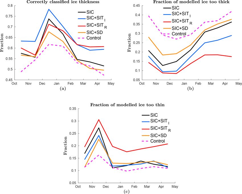
494                                                                      S. Fritzner et al.: The Metroms assimilation system

ECMWF numerical weather prediction (NWP) model (An-                a spatial resolution of 25 km and a 30-day average tempo-
dersen et al., 2006). To convert brightness temperatures to        ral resolution covering the entire Arctic. For the CryoSat-2
SIC a combination of the bootstrap and the Bristol algorithms      data set, no uncertainty estimates are provided; thus follow-
is used (Tonboe et al., 2016). The bootstrap algorithm is pri-     ing Zygmuntowska et al. (2014) an uncertainty of 0.5 m was
marily used for observations with low SIC, and the Bristol         used for all CryoSat-2 observations. Due to the low temporal
algorithm for high SIC. The older OSISAF products do not           coverage, this is most likely an underestimation of the un-
include an error estimate, but an estimate of the observation      certainty, and other publications have suggested higher un-
confidence. The observation confidences are a simple mea-          certainties (Xie et al., 2016; Chen et al., 2017). In our study,
sure of the observation quality, where 5 is excellent quality,     the main focus is on the impact of the observations on the
2 indicate poor quality, 1 indicates computation failure, and      assimilation system and thus a low error is applied in order
0 no data. In the more recent OSISAF observations, a total         to elucidate the model impact of the observations. Since the
uncertainty parameter is associated with each observation. In      CryoSat-2 data set is only valid for high-concentration ice, all
our study, the observation uncertainty of the OSISAF obser-        observations are in the internal part of the Arctic sea ice and
vations was given by the following formula:                        will in future also be referred to as internal ice thickness. The
                                                                   CryoSat-2 observations are only available in the cold season
TU = a + b · (5 − C),                                       (1)
                                                                   from October to April.
where C is the confidence and TU is the total uncertainty,             For thin SIT observations, the daily L3C SMOS Sea Ice
a = 0.06 and b = 0.1 are estimated based on the relation-          Thickness version 3.1 is used (Tian-Kunze et al., 2016).
ship between confidence and uncertainty in the more re-            These SIT observations are acquired from a satellite using a
cent OSISAF observations. Observations flagged with a con-         passive microwave with L-band frequency. Measurements of
fidence of 0 or 1 are not used in our study. For verifica-         brightness temperatures are converted into SIT using a radi-
tion of the modelled SIC, the ESA Sea Ice Climate Change           ation and thermodynamic model based on penetration depth
Initiative, Sea Ice Concentration Climate Data Record from         (Tian-Kunze et al., 2014). Xie et al. (2016) found that obser-
the AMSR-E and AMSR-2 Instruments at 25 km Grid Spac-              vations thinner than around 0.4 m were the most realistic to
ing, version 2.0 (Toudal Pedersen et al., 2017). The data set      use in the analysis. Hence, in this study, observations thicker
consists of satellite observations from the National Space         than 0.5 m have not been used. For the SMOS observations
Agency’s Advanced Microwave Scanning Radiometer in-                it is assumed that all observations are acquired at 100 % SIC;
struments (AMSR-E/AMSR-2). The AMSR-E/2 observa-                   thus the observations are assimilated as normalised ice vol-
tions are, like the OSISAF SIC observations, also based            ume. The SMOS data set has a resolution of 12.5 km and is
on measurements from a passive microwave measuring the             structured on a stereographic grid. Since all SMOS observa-
brightness temperature. The observations are structured on a       tions are thinner than 0.5 m they are all located in the vicin-
25 km grid. The OSISAF and AMSR-E/2 data sets are differ-          ity of the Arctic ice rim and will in future also be referred
ent data products, but are in many cases tuned to give similar     to as rim ice thickness. As for the internal ice thickness ob-
results and cannot be viewed as true independent data sets.        servations, the SMOS SIT are only available in the cold sea-
The AMSR-E/2 product has a gap from October 2011, when             son from October to April. The SMOS observations include
AMSR-E failed, to July 2012, when AMSR-2 became oper-              individual uncertainty estimates for each grid point. These
ational. This is in the middle of our analysis period, resulting   uncertainty estimates are a combination of uncertainties of
in less data for verification. The AMSR-E/2 SIC observation        measured brightness temperature, auxiliary data sets and as-
product includes individual uncertainty estimates for all grid     sumptions made in the radiation and thermodynamic mod-
points. This uncertainty is based on the sum of the algorithm      els. In general thicker ice has higher uncertainty (Kaleschke
uncertainty and smearing uncertainty. Smearing uncertainty         et al., 2017).
is related to the location of the observation compared to the          For verification of the modelled SIT, the weekly combined
grid.                                                              SMOS-CryoSat-2 data set version 1.3 was used (Ricker et al.,
   Two different SIT products are assimilated. For thick SIT       2017). This observation product provides SIT observations
observations, the CryoSat-2 Level-4 Sea Ice Thickness prod-        covering the whole Arctic during the cold season. In addi-
uct is used (Kurtz and Harbeck, 2017). The CryoSat-2 obser-        tion, the IceBridge L4 Sea Ice Thickness observations are
vations are based on radar altimeter measurements of sea ice       used for verification (Kurtz et al., 2013; Kurtz et al., 2014a).
freeboard. The SIT is derived assuming nominal densities for       This data set consists of SIT and snow-depth measurements
ice, snow and water and is only valid for high-concentration       from an aeroplane, using a radar altimeter measuring the ice
ice (> 70 %; Kurtz et al., 2014b); thus they are assumed to be     freeboard. The IceBridge observations are limited temporally
observations of thick ice relative to the SMOS observations.       to March–April, and spatially to parts of the Beaufort Sea, the
The snow depth used to calculate sea-ice elevation is con-         Canadian Archipelago and north of Greenland.
structed from the Warren climatology of snow depth (Warren             The snow-depth observations are derived from AMSR-E/2
et al., 1999), modified to account for the loss of multi-year      observed brightness temperatures (Rostosky et al., 2018).
ice in recent years (Kurtz and Farrell, 2011). The data set has    The data are available on a daily basis with a resolution

The Cryosphere, 13, 491–509, 2019                                                        www.the-cryosphere.net/13/491/2019/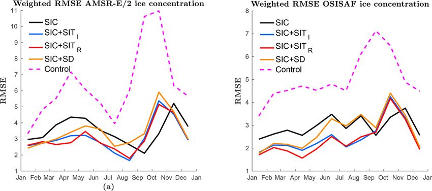
S. Fritzner et al.: The Metroms assimilation system                                                                           495

of 25 km × 25 km. The algorithm uses the same technique            The model background and analysis state vectors are matri-
which was developed by Markus and Cavalieri (1998) to re-          ces given by, xb ∈ Rn×N and xa ∈ Rn×N , respectively. Here
trieve snow depth over Antarctic sea ice. Their product is         n is the number of variables (that will become updated) times
based on an empirical relationship between the gradient ratio      number of grid cells, and N is the number of ensemble mem-
of the 37 and 19 GHz brightness temperature observations           bers. The covariance of the observations is given by R ∈
and Antarctic snow depth. It was adapted to retrieve snow          Rm×m , where m is the number of observations, H ∈ Rm×n
depth on Arctic sea ice (Comiso et al., 2003), but due to the      is the observation operator, which is a transformation opera-
radiometric properties of Arctic multi-year ice, the retrieval     tor between model and observation space, and y ∈ Rm×N is
is limited to first-year ice only. The new product by Ros-         the observation matrix. For the EnKF, the background error
tosky et al. (2018) makes use of lower frequency channels          covariance matrix, Pb , is estimated based on the covariance
(i.e. brightness temperature observations at 6.9 GHz) which        of an ensemble of model states. The ensemble is generated
are less sensitive to the Arctic multi-year ice and thus the re-   by either perturbing the forcing, the model parameters, the
trieval can be, with some exceptions (Rostosky et al., 2018),      observations or a combination of the three. The estimator for
applied over the whole Arctic sea ice. The new snow-depth          background error covariance, Pb ∈ Rn×n , is
retrieval was trained and evaluated using NASA’s Operation
IceBridge airborne snow-depth observations (Newman et al.,         Pb = ((xb − xb )(xb − xb )T ).                             (3)
2014). Those observations are, however, mainly limited to
March and April and, so far, no evaluation of the snow-depth          The overbars indicate an ensemble average. In our study,
product exists for the remaining winter season. We, therefore,     the deterministic ensemble Kalman filter (DEnKF) proposed
limit our analysis to snow-depth observations in March and         by Sakov and Oke (2008) is used. This method solves the
April. For the snow-depth product, uncertainty estimates ex-       analysis equation without the use of perturbed observations.
ist for every grid point. There are two main sources of uncer-        When using the EnKF spurious covariances might occur
tainty in this observation product: the first is that the number   due to distant state vector elements and insufficient model
of IceBridge observations used to develop the empirical re-        rank when small ensemble sizes are used. These artefacts
lationship between brightness temperatures and snow depths         can be reduced by using a method for localisation (Evensen,
is small compared to the coverage of the product. The sec-         2003; Sakov and Bertino, 2011), limiting the assimilation to
ond uncertainty is in the input parameters (brightness tem-        affect a smaller area. There are several methods for localisa-
perature, ice concentration, etc.). More on how the uncer-         tion, and in this study, the polynomial taper function (Gaspari
tainties are explicitly calculated can be found in Rostosky        and Cohn, 1999) is used. The taper function is a bell-shaped
et al. (2018). When the model simulations were performed,          function providing stronger influence on nearby grid cells.
the snow-depth product was in its early development state.
                                                                   4.2   Ensemble spread
Now, a slightly updated version of the snow-depth product
exists, but since the overall differences between the updated      Sufficient ensemble spread is essential for a robust and well-
version and the early state version are small we do not expect     functioning EnKF assimilation system. In general, this is
the updated data set to yield substantially different results.     maintained by the Kalman Filter equations, but it is impor-
   In addition to the radar observations, ice mass balance         tant to also take into account the uncertainty in the model
(IMB) buoy observations of SIT and snow depth (Perovich            and the atmospheric forcing. The atmospheric forcing is per-
et al., 2018) are used for model verification. These data in-      turbed to account for uncertainty in the forcing. The atmo-
clude measurements of SIT and snow depth from drifting             spheric forcing is perturbed using smooth pseudo-random
buoys in the Arctic at multiple time intervals and different       fields (Evensen, 2003) with zero mean and standard devia-
locations every year. The measurements are performed by            tion based on perturbation values applied also in the more
sounders (Polashenski et al., 2011).                               tested and robust TOPAZ system (Sakov et al., 2012). For the
                                                                   2 m temperature, the standard deviation is 3 K, cloud cover is
                                                                   20 % and per-area precipitation flux is 4 × 10⁻⁹ m; and for
4     Methods and model setup
                                                                   wind, 1 m s−1 in both horizontal directions is applied. To ac-
4.1    The ensemble Kalman filter                                  count for model uncertainty, the ice strength parameter, P ,
                                                                   is perturbed. This is done by perturbing the model parame-
The ensemble Kalman filter (EnKF) is a sequential data-            ter Cf which is the frictional energy dissipation parameter.
assimilation method used in a wide variety of geophysi-            In CICE, Cf is proportional to the ice strength (Hunke et al.,
cal systems (Evensen, 1994, 2009; Houtekamer and Zhang,            2015b),
2016). The analysis equation for the EnKF is given by
                                                                   P ∝ Cf .                                                   (4)
(Jazwinski, 1970; Evensen, 2003)
                                  −1                               The default value of Cf is 17, but according to Flato and
xa = xb + Pb HT       HPb HT + R         (y − Hxb ) .       (2)    Hibler (1995) this is not a well-known parameter. In our

www.the-cryosphere.net/13/491/2019/                                                        The Cryosphere, 13, 491–509, 2019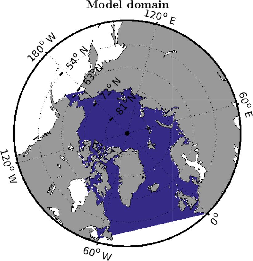
496                                                                          S. Fritzner et al.: The Metroms assimilation system

study, this parameter is modelled as a stochastic variable with      Table 1. Overview of the five experiments used to assess observa-
a mean value of 17 and a standard deviation of 10. The dif-          tion impact. The X marks a given observation that is assimilated in
ferent values are chosen based on values found during model          the experiment.
tuning using observations by Flato and Hibler (1995). Since
only one value less than 10 was found in their study, values                                   OSISAF    CryoSat-2    SMOS      Snow
less than 10 for Cf are not used.                                                                                               depth
                                                                         Exp1 (SIC)              X
                                                                         Exp2 (SIC + SITI )      X           X
4.3   Experimental design                                                Exp3 (SIC + SITR )      X                       X
                                                                         Exp4 (SIC + SD)         X                                X
The assimilation model system consists of 20 ensemble                    Exp5 (Control)
members, with an assimilation time step of 7 days. Simi-
larly to Sakov et al. (2012) a localisation radius of 300 km is
used. The initial ensemble is generated from ice states from         the sea ice, and because it is implemented consistently for all
1 January based on 20 different years of a stand-alone sea-          the model experiments.
ice model run without assimilation. The stand-alone model               Five experiments assimilating different observations are
was initialised without ice in 1979. All initial ocean states        used to investigate the effect of observations on the model.
are model output at the initial date 1 January 2010. This out-       In experiment 1 only OSISAF SIC is assimilated, in experi-
put is taken from a model spin-up over 1993–2010. Before             ment 2 both OSISAF SIC and CryoSat-2 SIT, in experiment 3
performing the experiments, a model system assimilating ice          both OSISAF SIC and SMOS SIT, in experiment 4 OSISAF
concentration and sea-surface temperature (SST) from OS-             SIC and snow depth (SD) observations, and experiment 5 is
TIA (Donlon et al., 2012) is run for 1 year until 1 Jan-             a control run without assimilation. All assimilation systems
uary 2011, to be used as an initial state.                           are initialised after 1 year of initial assimilation on 1 Jan-
   In the CICE model, the sea-ice variables are distributed          uary 2011 and run for 3 years. A summary of the different
into 5 thickness categories, while all observations are sin-         experiments is shown in Table 1.
gle category values. This discrepancy was solved by assim-
ilating the aggregated category values and using the EnKF
correlation properties to update each category individually.         5     Results
After assimilations, the analysis results are post-processed
                                                                     In this section, the output of the five ensemble experiments
before new forecasts are run. During post-processing, it is
                                                                     is compared. All results are based on the output from 2011
verified that the consistency of the different ice variables is
                                                                     to 2013. As mentioned, the first year of modelling, 2010, is
maintained during assimilation, as the analysis can lead to,
                                                                     only used to spin-up the experiments, generating a stable and
for instance, situations in which some areas have a positive
                                                                     consistent ice–ocean model state.
partial SIC but the corresponding partial SIT is zero or less
                                                                        Many of the results shown in this section will be based
than zero – in this example the SIC is set to zero. In addition,
                                                                     on the root mean squared error (RMSE). In this study, the
all variable bounds are checked during post-processing. Due
                                                                     RMSE is weighted by the observation uncertainty, σObs(i) ,
to linear correlation effects of the EnKF, locations with non-
physical concentrations can occur, for instance, SIC values
                                                                               v
                                                                               u N
                                                                               u P (Mod(i)−Obs(i))2
both above one and below zero.                                                 u            2
                                                                               t i=1       σObs(i)
   For the ocean parameters, only ocean temperature and              RMSE =                           ,                         (5)
ocean salinity are updated during the assimilation. Experi-                                N
ments have shown that large instantaneous changes to the             where N is the number of grid cells, Obs and Mod are the
ocean parameters lead to model instability. These large              observations and model values, respectively. Thus, an RMSE
changes are especially seen in the marginal ice zone (MIZ),          of 1 indicates that the difference between model and obser-
where the ensemble spread is largest and the update to the           vations are on average of the same order as the observation
ensemble is strongest. To prevent these instabilities in the         uncertainty.
ocean, the magnitude of the ocean update during an assim-
ilation step is limited. In this work, a maximum temperature         5.1     Validation against concentration observations
update step of 0.2 K for the ocean surface layer and 0.1 K for
all other ocean layers is chosen. Similarly, for the salinity, 0.2   In Fig. 2 the monthly averaged ensemble mean of the five ex-
for the surface layer and 0.1 for all other layers is chosen. The    periments were validated against two different SIC observa-
limits are chosen crudely, based on values where the model           tion products; one assimilated and one independent are plot-
did not immediately crash after assimilation. Although this is       ted. In Fig. 2a the RMSE values of the ensemble mean of
a crude simplification, almost omitting the ocean update, it is      the modelled SIC validated with the observed AMSR-E/2
believed to be sound, because the focus in this research is on       product are plotted after assimilation. All four assimilation

The Cryosphere, 13, 491–509, 2019                                                             www.the-cryosphere.net/13/491/2019/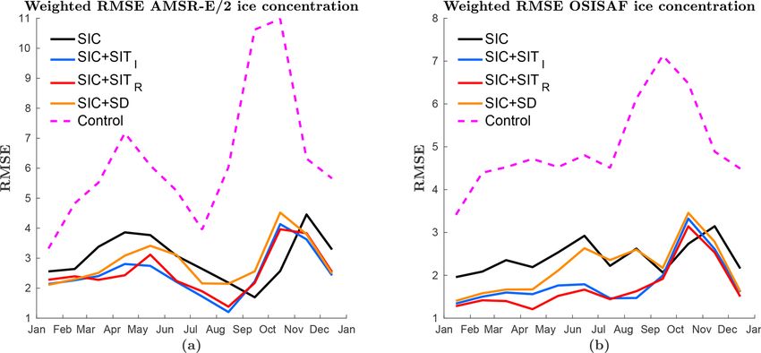
S. Fritzner et al.: The Metroms assimilation system                                                                               497

Figure 2. The monthly averaged RMSE of the ensemble mean SIC over 3 years. In (a) the model is validated against AMSR-E/2 SIC
observations and (b) OSISAF SIC observations. The lines represent different experiments: black is only SIC assimilation, blue is SIC
and CryoSat-2 thick internal SIT assimilation, red is SIC and SMOS and thin rim SIT assimilation, yellow is SIC and snow-depth (SD)
assimilation and magenta dotted is without assimilation.

experiments are found to be significant improvements com-            icantly better than the OSISAF SIC-only experiment. When
pared to the control experiment without assimilation. Using          compared to the OSISAF observations, the snow-depth as-
a one-sided paired sample student t test over all 36 months of       similation experiment is also found to be significantly better
simulation, both the CryoSat-2 internal SIT and SMOS rim             than the OSISAF SIC-only experiment: there are significant
SIT experiments show significant improvements compared               differences, especially during the first half of the year. In con-
to the OSISAF SIC-only experiment on a 5 % level, but the            clusion, assimilating SIT and to some degree, snow depth has
differences are relatively small. The significance is derived        a significant effect on the SIC RMSE, and the effect is largest
using monthly data, but not yearly averaged data as in the           for the first half of the year. In the transition from melting ice
figures. However, the snow experiment is not found to be sig-        to freezing ice, all four experiments give similar high RMSE
nificantly better than the OSISAF SIC-only experiment on a           values.
5 % level: a p value of 0.23 is found. The difference between           RMSE estimates are sensitive to individual measurements,
the SIT experiments and the SIC-only experiment is largest           contributing to large portions of the total RMSE; thus, a small
during the first half of the year, while in the second half of       area with large errors will obscure the overall model results.
the year all experiments give similar results with a peak in         Another assimilation quality measure is hit rates, where all
the RMSE in October–November. This peak in RMSE is also              grid cells are given equal weight in the analysis. In our work,
seen in the control model, indicating a possible model prob-         the hit rate is analysed by classifying the SIC in three cate-
lem related to the transition from the melt season to the grow-      gories: open water (concentration less than 10 %), low con-
ing season.                                                          centration (< 50 %), and high concentration (> 50 %). The
   In Fig. 2b the monthly averaged RMSE of the model SIC             hit rate is defined as the number of grid cells correctly classi-
ensemble mean versus the assimilated OSISAF SIC observa-             fied. The independent AMSR-E/2 observations are used for
tions is plotted. The result in Fig. 2b is similar to that of (a),   verification. In Fig. 3a the number of grid cells correctly clas-
but the differences between the models are larger when veri-         sified is shown; in Fig. 3b the number of grid cells with mod-
fied against OSISAF, even though the OSISAF observations             elled ice and observed water are shown; in Fig. 3c the number
are assimilated in all experiments. This is partly related to the    of grid cells with modelled water and observed ice are shown;
lower observation error in the MIZ for the OSISAF data set           in Fig. 3d the number of grid cells with a wrong concentra-
than for the AMSR-E/2 data set, and the OSISAF including             tion category are shown, with high SIC classified as low SIC
almost an extra year of observations due to the AMSR-E/2             and vice versa. All assimilation experiments outperform the
gap. Since the RMSE values are weighted by the observation           control run in terms of hit rate. The control run has a large
error the differences in the MIZ are more pronounced when            number of false positives, indicating too much ice. Among
verified against OSISAF SIC observations. In addition, ev-           the experiments, the variations are small in spring, autumn
idence that there are small differences between the two ob-          and winter, while summer shows significant differences. In
servation products is seen by different shapes on the graphs,        summer all experiments have a minimum, which is related to
even though the curves follow the same trends. As men-               an underprediction of sea ice and wrong classification of con-
tioned, the CryoSat-2 and SMOS SIT experiments are signif-           centration in observations due to melt ponds on ice, which

www.the-cryosphere.net/13/491/2019/                                                           The Cryosphere, 13, 491–509, 2019
498                                                                      S. Fritzner et al.: The Metroms assimilation system

leads to an underestimation of SIC in the observations (Kern       Table 2. The March–April averaged RMSE values of the five ex-
et al., 2016). In summer the CryoSat-2 assimilation has the        periments compared to the IceBridge aerial SIT observations. Bold
highest number of hits, closely followed by the SMOS and           values represent the model with the lowest RMSE values for that
snow experiments.                                                  year.

5.2   Total extent and volume                                                                2011    2012   2013    2011–2013
                                                                       SIC                    0.88   0.87    1.11          0.94
In Fig. 4, the total sea ice extent (Fig. 4a), the total sea-ice       SIC+SITI               0.63   0.86    0.72          0.80
volume (Fig. 4b), and the total sea-ice volume overlapping             SIC+SITR               0.74   1.14    0.87          0.96
the area and period covered by the CryoSat-2 internal SIT              SIC+SD                 0.93   1.38    1.64          1.51
observations (fig. 4c) are shown for the five experiments. Fig-        Control                0.82   1.25    2.31          1.38
ure 4a shows that the control experiment has a too large sea-          Cryo observations      0.67   0.95    0.84          0.84
ice extent both in summer and winter, while the assimilation
experiments have a slightly too large ice extent in winter.
   The total sea-ice volume shown in Fig. 4b indicates large       experiments. The other three experiments are more similar,
differences between the five experiments. Snow depth assim-        all showing high RMSE values. It is found using a one-sided
ilation generally leads to thicker ice. The model has a lower      paired student t test that only the SMOS SIT experiments
amount of snow than the observations, and due to a posi-           are significantly better than the SIC-only assimilation, with
tive correlation, the ice thickness is also increased during the   p values less than 5 %. Due to the high RMSE values, only
assimilation of snow depth. The increased thickness can be         small improvements are seen compared to the control run.
seen by the fact that the snow-depth experiment has about          The result is consistent with what was found for the sea-ice
the same extent as the other experiments, but shows a sig-         volume (Fig. 4c), regarding the SMOS SIT assimilation hav-
nificantly larger ice volume, both in summer and winter for        ing the strongest effect on the modelled SIT. The reason for
all 3 years. Both the SMOS and CryoSat-2 ice thickness ex-         the high RMSE values is that, in general, the model has too
periments lead to thinner sea ice compared to the control ex-      much ice, leading to too thick ice in the MIZ. For the SMOS-
periment. In particular, the SMOS assimilation model shows         CryoSat-2 SIT product, the uncertainties provided are very
much thinner sea ice than the other assimilation experiments.      small, especially in the MIZ where the SMOS observations
The thin SIT observations have a very strong effect on the         are used; thus when calculating the RMSE these values have
modelled SIT, seen by an abrupt update of sea-ice volume           a huge effect on the result. Thus, it is also reasonable that
during assimilation in winter. A concerning effect of the as-      the assimilation system for these MIZ-thickness observations
similation experiments is the strong decrease in the Arctic        also gives the lowest RMSE values. For the other assimila-
sea-ice volume throughout the period of study. The sea-ice         tion systems, the ice extent is updated in the MIZ, but the
volume maximum in winter decreases for every year of as-           thickness reduction takes longer because it has to evolve over
similation; this is not seen in the control run.                   time.
   In Fig. 4c the modelled sea-ice volume is compared to the          As for the SIC observations, the RMSE values are bi-
sea-ice volume in the combined CryoSat-2-SMOS product.             ased by locations showing large differences. Particularly for
The control model is found to have too thick ice compared          thickness which is not bounded upwards, a few grid cells in
to the observations, while the experiments assimilating SIT        the MIZ can contribute to a large total RMSE. As for con-
are much closer to the observations, though largely biased.        centration, an alternative measure is one in which correctly
This can be used to explain the drastic decrease in sea-ice        classified model thickness hit rates are used. The model is
volume found in Fig. 4b. The model SIT is adjusting to the         separated into four thickness categories: less than 0.5 m, be-
observations by rapidly thinning the sea ice. For the OSISAF       tween 0.5 and 1.5 m, between 1.5 and 3 m, and above 3 m. In
SIC-only assimilation experiment, the volume is also slowly        Fig. 6a the number of correctly classified ice thicknesses grid
diverging towards the observed volume, even though SIT is          cells is plotted for each experiment. The figure shows that
not assimilated. This is likely related to a more accurate sea-    the CryoSat-2 internal SIT experiment is the model which
ice extent that also leads to improved ice thickness in the        has the highest number of correctly classified grid cells.
marginal ice zone. However, the improvements are obtained          The other experiments are more similar, except in spring
at a slower pace than when assimilating SIT directly.              where the SMOS rim SIT assimilation is equally good as
                                                                   the CryoSat-2 internal SIT assimilation, and both are much
5.3   Validation against thickness observations                    better than the other three. In spring the SIC-only and snow-
                                                                   depth assimilations are not improved compared to the control
In Fig. 5a the SIT RMSE of the ensemble mean modelled SIT          case. In general, the model shows too much ice. This can be
is verified with the combined SMOS-CryoSat-2 SIT prod-             seen by a large number of grid cells having too thick ice in the
uct. The experiment assimilating SMOS thin SIT has signif-         control model (Fig. 6b). This is a combination of the sea-ice
icantly lower RMSE values than the other three assimilation        extent being too large and the ice being too thick. By assim-

The Cryosphere, 13, 491–509, 2019                                                          www.the-cryosphere.net/13/491/2019/
S. Fritzner et al.: The Metroms assimilation system 499
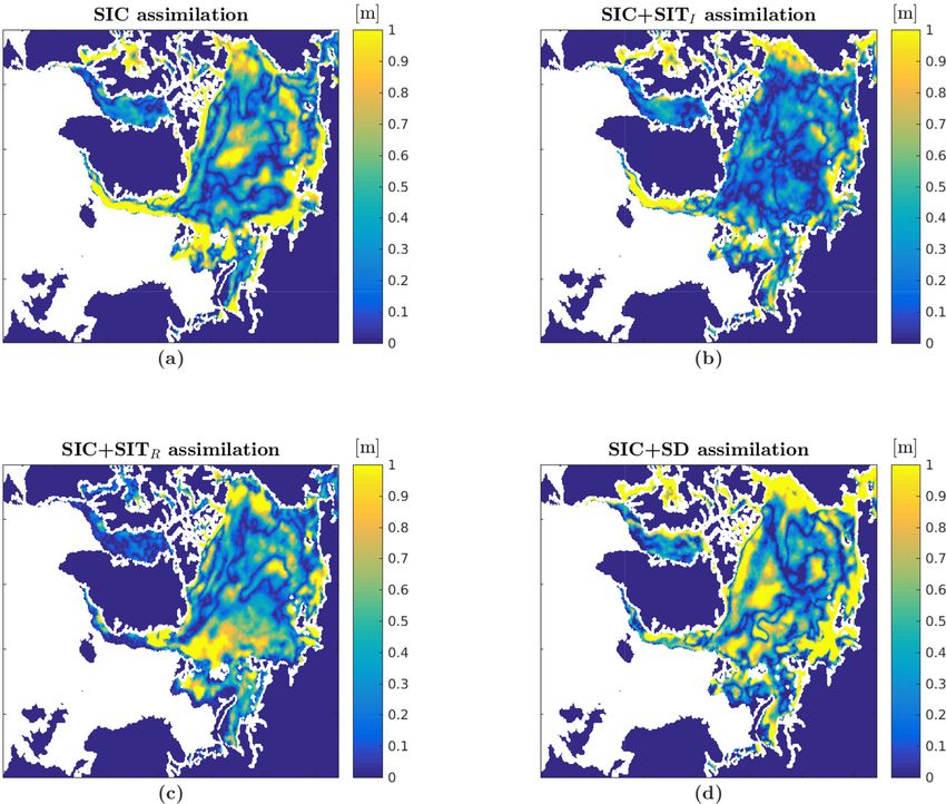
Figure 3. Classification of the model result based on three classes: high-concentration ice (> 50 %), low concentration ice (< 50 %) or water
and compared to AMSR-E/2 SIC observations. The figures show (a) the fraction of correctly classified grid cells, (b) the fraction of grid cells
with modelled ice while water is observed, (c) the fraction of grid cells with modelled water while ice is observed, and (d) fraction of grid
cells where the model and observations have different SIC classification. The colour coding in the figure is the same as that of Fig. 2. These
panels cover all possible classifications; thus the sum of them equals one.
ilating the observations, the ice volume is reduced, not only rior. This shows that assimilating SIT is important both in the
for the SIT assimilations, but also for the snow-depth and interior and in the MIZ.
SIC-only assimilations, but to a lower degree for the latter. In addition to the satellite observations, the independent
This is an effect of a lower sea-ice extent (Fig. 4a). In Fig. 6c airborne IceBridge data set is used for verification of the
the number of grid cells with too thin ice compared to the ob- modelled SIT (Kurtz et al., 2013; Kurtz et al., 2014a). This
servations is shown. It was found that this is a big problem in data set has low temporal and spatial distributions, but is be-
early winter for all experiments but reduces during winter for lieved to have higher accuracy and much higher spatial and
all experiments except the SMOS experiment. During SMOS temporal resolutions. All observations occurring in March
assimilation, only thin ice is assimilated, which might lead to and April are gathered as a yearly averaged observation as
a bias towards the thinner ice, causing a relatively high num- a function of space. These yearly observations are then com-
ber of grid cells with too thin ice. pared to modelled SIT averaged over the same period for the
As an example, in Fig. 7 the absolute differences be- observed IceBridge locations. Since the IceBridge resolution
tween the experiments and the combined CryoSat-2 SMOS is much higher than that of the model, all IceBridge obser-
ice thickness observations are plotted for 1 April 2011. Fig- vations within one model grid cell are averaged and used
ure 7 is consistent with Fig. 6a, showing that the CryoSat-2 for verification. The average is done by a weighted mean
experiment has the smallest differences compared to the ob- based on the observation uncertainty. The validation results
servations in the internal Arctic, affecting a large area; how- are shown in Table 2. On average, the CryoSat-2 SIT exper-
ever, large differences can be seen in MIZ. While for the iment has the best SIT estimation as compared to IceBridge.
SMOS rim SIT assimilation the effect is the opposite, with Both the SMOS and the CryoSat-2 SIT experiments give on
a large impact in the MIZ and small impact in the ice inte- average thinner SIT than the IceBridge observations, which
are consistent with the findings of Chen et al. (2017). The
www.the-cryosphere.net/13/491/2019/ The Cryosphere, 13, 491–509, 2019500 S. Fritzner et al.: The Metroms assimilation system Figure 4. The evolution of (a) total sea-ice extent, (b) total sea-ice volume and (c) total sea-ice volume for the area covered by the CryoSat- 2-SMOS SIT observation product. The coloured lines represent the same as in Fig. 2. In (a) the black stars represent the AMSR-E/2 SIC observations and the red stars the OSISAF SIC observations. In (b) same as (a) without observations. In (c) the black stars represent the CryoSat-2-SMOS observation product. The x label is given as month and year. last line in the table shows the RMSE between the CryoSat-2 values, the RMSE is calculated on the 7-day ensemble mean observations and the IceBridge observations and the results and averaged for each year. Since SIT is a relatively slow show that the error is comparable to the model errors. varying variable, for each 7-day output, observations from For all 3 years, the CryoSat-2 assimilation has lower ±3 days are used to increase the number of observations. The RMSE values than the CryoSat-2 observations, indicating a IMB observations do not include an uncertainty estimation; well-balanced assimilation, with appropriate observation er- hence the RMSE is not normalised as was the case for other ror and ensemble spread. It should also be mentioned that the RMSE estimates in this work. The results show that over the CryoSat-2 observations have less spatial coverage than the 3 study years, the SMOS internal SIT assimilation system has model and not all IceBridge observations are covered; thus the lowest RMSE values, followed by the CryoSat-2 internal the number of useful observations for the CryoSat-2 RMSE SIT assimilation. The other three show similar results, again calculation are smaller than for the validation of the experi- indicating a positive impact of assimilating ice thickness in ments. the model. Another independent data set of SIT observations comple- menting the IceBridge observations by a temporal resolution 5.4 Validation against snow observations spanning the entire year is the IMB buoy data set. The re- sult of model validation with the IMB product is shown in In Fig. 5b the RMSE of monthly averaged modelled snow Table 3. For these observations, a slightly different method depth is plotted over all ensembles validated against the ob- than that applied for IceBridge is performed. This is because served satellite snow depth (Rostosky et al., 2018) used for IceBridge temporarily only covered March–April, while the assimilation. The control experiment is found to have the IMB data span the entire year. The buoy observations are lowest RMSE values. This is most likely an effect of sea-ice converted to daily averages on the model grid. From these extent being different to the assimilation experiments, rather The Cryosphere, 13, 491–509, 2019 www.the-cryosphere.net/13/491/2019/
S. Fritzner et al.: The Metroms assimilation system                                                                                  501

Figure 5. RMSE of monthly averaged model SIT and snow depth averaged over all ensemble members for the years 2011–2013 calcu-
lated against the (a) combined SMOS-CryoSat-2 SIT product and (b) observed snow-depth product. These are observations also used for
assimilation. The colour coding is as in Fig. 2.

Table 3. The yearly averaged RMSE values of the five experiments     Table 4. The March–April-mean RMSE of the ensemble-mean
compared to the IMB SIT buoy observations. Bold values represent     snow depth averaged over all grid cells. The five experiments and
the model with the lowest RMSE values for that year. No uncertain-   the snow-depth satellite observations are compared to the IceBridge
ties are used to normalise the RMSE values.                          airborne snow-depth observations. Bold values represent the model
                                                                     with the lowest RMSE values for that year.
                      2011    2012    2013    2011–2013
        SIC           0.99    1.45     1.32          1.27                                     2011     2012    2013    2011–2013
        SIC+SITI      1.08    1.28     1.00          1.13                 SIC                  0.79    1.38     2.64          1.63
        SIC+SITR      1.09    1.07     0.99          1.05                 SIC+SITI             0.79    1.15     1.44          1.06
        SIC+SD        1.02    1.40     1.28          1.25                 SIC+SITR             0.78    0.83     1.73          1.17
        Control       1.46    1.27     1.23          1.26                 SIC+SD               0.74    1.22     1.46          1.13
                                                                          Control              0.77    2.49     1.85          1.33
                                                                          Snow observation     1.46     NA      1.17          1.16

than the assimilation declining the accuracy of the modelled            NA – not available

snow depth. In addition, the control experiment has an in-
creasing RMSE during the period, while the assimilation ex-
                                                                     only one snow layer, which may affect the snow cover accu-
periments show the effect of assimilation by decreasing the
                                                                     racy. It is also important to mention that the snow observa-
RMSE. For the assimilation experiments, the snow experi-
                                                                     tions are in an early development stage and might have larger
ment has the lowest RMSE values followed by the CryoSat-2
                                                                     uncertainties than those used in this study.
experiment, indicating that the thick ice observations have a
                                                                        Additional model verification is performed with the inde-
correlation effect on the snow depth. These two observation
                                                                     pendent IMB buoy snow-depth observations. The method of
products also cover a similar area of the Arctic Ocean.
                                                                     validation is performed in a similar manner as for SIT vali-
   A verification of the modelled snow depth using the in-
                                                                     dation with IMB buoy data: the results are shown in Table 5.
dependent IceBridge data set is given in Table 4. The same
                                                                     As the IMB data do not include an uncertainty these RMSE
method as for the SIT in Table 2 was used, where March–
                                                                     values are not normalised; thus they are significantly lower
April model values are compared to the IceBridge obser-
                                                                     than the error estimates from the ice bridge validation in Ta-
vations and averaged. It is found that none of the experi-
                                                                     ble 4. From the table it is clear that the differences between
ments are particularly better than any of others when ver-
                                                                     the assimilation systems are small. The assimilation systems
ified against IceBridge snow-depth observations. It is seen
                                                                     for snow depth and CryoSat-2 internal SIT are slightly bet-
that, within one grid cell, there are huge variations in the
                                                                     ter than the others, but the differences are too small to obtain
IceBridge snow observations. Such variations cannot be pro-
                                                                     conclusions.
vided with a coarse-resolution model. Hence, even though
IceBridge is used to “tune” the snow observations (Rostosky
et al., 2018), large RMSE values are estimated for the exper-
iment assimilating snow depth. In addition, the snow compo-
nent used in our coupled system is likely too simple, having

www.the-cryosphere.net/13/491/2019/                                                           The Cryosphere, 13, 491–509, 2019
502 S. Fritzner et al.: The Metroms assimilation system
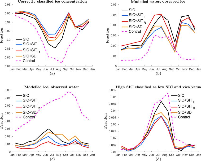
Figure 6. The monthly mean SIT averaged over all ensemble members is classified into four thickness categories and compared to the
CryoSat-2-SMOS SIT observation product. The fraction of grid cells are shown with (a) correctly classified thickness category, (b) too thick
ice, and (c) too thin ice. As in Fig. 2 the coloured lines represent different experiments.
Table 5. The yearly averaged RMSE values of the five experiments also gives the most accurate forecasts. Thus, the CryoSat-2
compared to the IMB snow-depth buoy observations. Bold values and SMOS SIT assimilation experiments have a better 7-day
represent the model with the lowest RMSE values for that year. No forecast from January to June than SIC only, and snow-depth
uncertainties are used to normalise the RMSE values. assimilation shows improvements from January to April. Us-
ing the OSISAF SIC observations (Fig. 8b) gave the same re-
2011 2012 2013 2011–2013
sult as found for AMSR-E/2: the best initial states also pro-
SIC 0.06 0.15 0.2 0.15 vide the best forecast, indicating that the sea ice does not
SIC+SITI 0.08 0.14 0.17 0.13 change much overall in a week. The same experiments were
SIC+SITR 0.09 0.15 0.17 0.14 also done for ice thickness and snow depth and similar re-
SIC+SD 0.09 0.14 0.16 0.13 sults were encountered. A reason for the small differences
Control 0.09 0.16 0.19 0.15 between the different experiments is the coarse model reso-
lution. Large-scale variations as seen by a 20 km model are
not expected within a week.
5.5 One week forecasts
Figure 8 shows the RMSE of the monthly averaged mod- 6 Seasonal forecast
elled SIC over all ensemble members before assimilation
validated against the AMSR-E/2 and OSISAF SIC observa- In the previous section, it was found that our coarse-
tions. Since the assimilation time step is 7 days, this gives resolution model only exhibits small changes during a 1
the accuracy of a 7-day forecast. The comparison against week forecast. Thus, a more interesting forecast would be
AMSR-E/2 SIC observations (Fig. 8a) shows that the dif- one of seasonal length. A 5-month forecast of the Septem-
ferences between the experiments are small, and the differ- ber sea-ice extent is performed. This is done by running
ences are similar to those found after assimilation (Fig. 2a). each of the experiments from mid-April to mid-September
In general, the system with the most accurate initial state each year without assimilation and validating them against
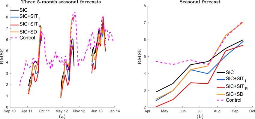
The Cryosphere, 13, 491–509, 2019 www.the-cryosphere.net/13/491/2019/S. Fritzner et al.: The Metroms assimilation system 503 Figure 7. Absolute differences between the experiments and the combined SMOS-CryoSat-2 observation product are given on 1 April 2011. The experiments are assimilating (a) OSISAF SIC, (b) OSISAF SIC and CryoSat-2 SIT, (c) OSISAF SIC and SMOS SIT and (d) OSISAF SIC and snow depth. Figure 8. RMSE of monthly averaged (over 3 years) ensemble mean of 7-day forecast SIC validated against (a) AMSR-E/2 SIC observations and (b) OSISAF SIC observations. the OSISAF SIC observations. The actual start date varied in late summer. In general, the model error is gradually in- slightly from year to year because of the 7-day assimilation creasing towards the level of the control run, and in sum- cycle, but the start date was the same for all experiments. In mer they have similar error levels. In August–September the Fig. 9a, the RMSEs of three 5-month forecasts are shown se- experiments assimilating thickness and concentration seem quentially, and a monthly averaged RMSE over the 3 years to be improved compared to those without assimilation and is shown in Fig. 9b. The figures show that the experiments assimilating snow-depth observations. All experiments show have very similar seasonal forecasts, with some differences an increased RMSE in 2013: this is related to a too low sea- www.the-cryosphere.net/13/491/2019/ The Cryosphere, 13, 491–509, 2019
504                                                                      S. Fritzner et al.: The Metroms assimilation system

ice extent. The low sea-ice extent is caused by weaker mod-        This is a consequence of too much ice in the control model,
elled ice growth compared to observations in the first months      causing the observed MIZ to be located deeper in the Arctic
of 2013.                                                           compared to the model, as noted by Fritzner et al. (2018).
   The seasonal forecast is compared to a climatological sea-         In the verification of modelled SIT (Fig. 5a), the SMOS
sonal forecast in Fig. 10. This provides an estimate of the        rim SIT assimilation was found to give the lowest RMSE
expected sea-ice forecast accuracy. The climatological ex-         values, while the CryoSat-2 internal SIT assimilation had
periment is done by running the model with averaged atmo-          the largest amount of correctly classified thickness grid cells.
spheric forcing data over the years from 2000 to 2014. The         This is as expected since, even though the CryoSat-2 obser-
result shows that the forecast skill of the model is rapidly de-   vations cover a larger area, they are 30-day averaged obser-
creasing and that a correct atmospheric forecast is very im-       vations with much larger uncertainties than the SMOS ob-
portant for an accurate sea-ice forecast. Still, skills are ev-    servations. In addition, the non-updated grid cells in the MIZ
ident on much longer timescales that can be obtained with          lead to larger RMSE values than non-updated grid cells in
numerical weather prediction models.                               the internal Arctic, where the model, in general, is more ac-
                                                                   curate and less sensitive to changes. When verified by Ice-
                                                                   Bridge observations, which only cover the central Arctic, the
7   Discussion                                                     CryoSat-2 SIT assimilation experiment was found to give the
                                                                   lowest SIT RMSE values. The CryoSat-2 SIT observations
Significant differences in modelled SIC after assimilation         are in general thinner than the SIT values for the SIC-only
was found, especially in the first half of the year. The SMOS      experiment. In comparison with the IceBridge observations,
and CryoSat-2 SIT assimilations gave the lowest RMSE val-          the CryoSat-2 SIT is biased low, which was also found by
ues, which are significantly better than when assimilating         Chen et al. (2017). When assimilating snow depth, it was
OSISAF SIC-only. The snow-depth experiment showed im-              found that snow-depth observations, in general, were thicker
provements during the first half of the year compared to the       than those modelled, resulting in increased snow depth dur-
experiment assimilating OSISAF SIC observations only. In           ing assimilation. Due to the correlation nature of the EnKF,
addition, assimilating SIT and snow depth lead to an im-           a positive correlation between snow depth and SIT resulted
proved model of SIC in summer, where the CryoSat-2 in-             in increased SIT in the snow-depth assimilation experiment
ternal SIT assimilation gave the highest number of correctly       compared to the other assimilation experiments.
classified grid cells, closely followed by the SMOS rim SIT           Validating our experiments with snow observations proved
and snow-depth assimilations. The reason for these differ-         the control run to have the lowest RMSE values. This can be
ences in summer is that the pace at which the ocean becomes        an effect of different sea-ice extents in the control run than
ice-free is dependent on the ice thickness and the snow depth.     in the assimilation experiments. For the control model, the
In the second half of the year, autumn and early winter, all       ice extent is too large, thus collecting more snow on the ice
our experiments gave similar results. These similarities seem      than the assimilation experiments. When the ice concentra-
to be a consequence of the transition from melt season to          tion is reduced during assimilation, the accumulated snow is
growing season not being well represented in the model. The        also removed, which can result in the removal of too much
observed transition is faster than the modelled, leading to an     snow if the ice extent is less than it should be. A verification
extended period with more open water in the model than in          of the impact of assimilation on the snow depth is that the
the observations.                                                  RMSE is decreasing throughout the observation period for
   In the control model without assimilation, the ice extent       the assimilation experiments, while for the control run the
both in summer and winter was found to be larger than              RMSE is increasing. Between the assimilation experiments,
observed. However, with assimilation, the experiments are          the snow-depth assimilation was found to give the lowest
closer to the observed extent, even though a slight overes-        snow-depth RMSE values, which is not unexpected since the
timation of extent in winter was found for the first 2 years.      same data set is used for assimilation and verification. More
The sea-ice extent overestimation in winter is a result of a       interestingly the CryoSat-2 internal SIT experiment has sig-
lower effect of SIC assimilation in winter due to lower en-        nificantly lower RMSE values than the SMOS rim SIT and
semble spread. When the ensemble spread is low the EnKF            OSISAF SIC-only assimilations, indicating a close correla-
assimilation result is closer to the model values, because the     tion between SIT and snow depth. A curiosity here is that
estimated model errors become small.                               the SIT assimilation has a positive effect on the snow depth,
   It is found that originally the sea-ice volume is too large     while it was found previously that the snow-depth assimila-
compared to the observations, and over the 3 years, the sea-       tion had a negative effect on the SIT. This is likely an ef-
ice volume in the assimilation experiments are gradually de-       fect of more SIT observations than snow-depth observations,
creasing towards the observed values in the SMOS-CryoSat-          and SIT is assimilated throughout the whole winter. It could
2 SIT product. The effect is much stronger for the SMOS            be the case that the correlation relationship between snow-
rim SIT assimilation, indicating that a large portion of the       depth and SIT changes throughout the winter. This results
original sea-ice volume overestimation is located in the MIZ.      in a better snow-depth estimate for SIT assimilation, while

The Cryosphere, 13, 491–509, 2019                                                       www.the-cryosphere.net/13/491/2019/
You can also read