Implicit Diversity in Image Summarization
←
→
Page content transcription
If your browser does not render page correctly, please read the page content below
Implicit Diversity in Image Summarization
                                                                    L. Elisa Celis1 and Vijay Keswani2
                                                                                1
                                                                              Yale University
                                                 2
                                                     École Polytechnique Fédérale de Lausanne (EPFL), Switzerland
arXiv:1901.10265v1 [cs.LG] 29 Jan 2019

                                                                               January 30, 2019

                                                                                    Abstract
                                             Case studies, such as [19] have shown that in image summarization, such as with Google
                                         Image Search, the people in the results presented for occupations are more imbalanced with
                                         respect to sensitive attributes such as gender and ethnicity than the ground truth. Most of the
                                         existing approaches to correct for this problem in image summarization assume that the images
                                         are labelled and use the labels for training the model and correcting for biases. However, these
                                         labels may not always be present. Furthermore, it is often not possible (nor even desirable) to
                                         automatically classify images by sensitive attributes such as gender or race. Moreover, balancing
                                         according to the labels does not guarantee that the diversity will be visibly apparent – arguably
                                         the only metric that matters when selecting diverse images.
                                             We develop a novel approach that takes as input a visibly diverse control set of images
                                         and uses this set to produce images in response to a query which are similarly visibly diverse.
                                         We implement this approach using pre-trained and modified Convolutional Neural Networks
                                         like VGG-16, and evaluate our approach empirically on the Image dataset compiled and used
                                         by [19]. We compare our results with the Google Image Search results from [19] and natural
                                         baselines and observe that our algorithm produces images that are accurate with respect to
                                         their similarity to the query images (on par with that of the Google Image Search results), but
                                         significantly outperforms with respect to visible diversity as measured by their similarity to our
                                         diverse control set.

                                                                                         1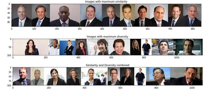
Figure 1: A simple post-processing approach for ensuring diversity in image search. A small “di-
versity control set” of images is taken as input, and (relevant) images are assigned a similarity score
with each image in the control set. These scores are combined with the similarity scores provided
in a black-box manner using an existing image search approach. A simple ranking algorithm then
selects the final images using this combined score.

1     Introduction
The last decade has seen a rise in popularity and usage of various image generation and classification
algorithms. Along with that, we also have detailed image datasets that have been manually or
automatically annotated with rich features. Given the availability of these image datasets, one of
the directions of research that is pursued is to develop algorithms that can identify images with
similar context. For example, given a huge image dataset of people at work, can we identify a
subset of images of people who are doctors by occupation? Algorithms based on feature extraction
algorithms and services such as Google Image Search already perform image summarization by
responding to a query with an appropriate set of images. However, as shown by case studies such
as [19], Google Image search is often biased with respect to sensitive attributes of the data such as
gender and ethnicity – if overrepresent the majority demographics of the given queries.
    The presence of these biases can be very harmful, considering the wide usage of such algorithms.
[19] showed that, similar to other forms of media, gender bias in image search results of occupations
leads to an incorrect perception of the number of women within the queried occupation. Further-
more, the use of the results from biased algorithms can also lead to “feedback loops”, wherein the
use of the biased results can be propagated to or even reinforced by other tools trained on these
results. For example, [22] showed through simulations of predictive policing tools that due to the
bias in training data, the tools suggest increased policing in black neighbourhoods. Similarly, [10]
showed that women are shown fewer online ads of high paying jobs than men.
    To prevent such scenarios in case of image classification tasks, it is important to ensure that
the algorithms used for image summarization are unbiased or represent the ground truth. To that
end, our goal is to provide a simple image ranking and summarization algorithm which can ensure
that the returned images correspond to the query yet are also visibly diverse.

1.1   Our Contribution
For a dataset of images, we provide a simple algorithm that, given a query, returns a small set of
images that correspond to that query and are “visibly diverse” (Section 2). The algorithm takes as
input a small control set of diverse images that is completely independent of the query. We take any
image matching tool as a blackbox to obtain a score of similarity between a pair of images. In that

                                                  2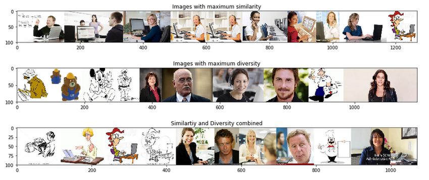
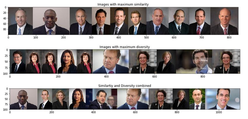
(a) CEOs                                         (b) Doctors

Figure 2: Top images returned by the algorithm for query occupations CEOs and Doctors. The
first row shows images with maximum similarity score, the second row shows images with best
diversity score and third one shows images with best combined scores.

sense, our algorithm can be considered a post-processing algorithm, that given an image similarity
scoring algorithm and a diversity control set, can be used to ensure that the images returned are
accurate and diverse.
    Each image is given a query similarity score which corresponds to how well it represents the
desired query. The candidate images are also given a similarity score with respect to each image in
the diversity control set using the image matching tool. After adding the query similarity score to
the similarity score with respect to the diversity control set, we rank the images by the combined
score for each image in the control set and output the ones with the best scores.
    In this paper, since we do not have access to extra information about the images in the dataset,
we use CNN-based feature extraction and image matching techniques to accomplish the goal (Sec-
tion 2). We test the algorithm on the dataset compiled by [19]. The dataset consists of top Google
images results for around 96 queried occupations, which they used to show the existence of gender
bias in these results (Section 4.1). We show that our algorithm returns much more gender-balanced
results than Google image search results (Section 4.2). Furthermore, we show that it can also
increase the visible racial diversity of the image search results.
    To the best of our knowledge, this is the first algorithm that does not use explicit labels to
ensure diversity in image summarization. Furthermore, depending on the robustness of the feature
extractor, our algorithm can be used to ensure that the returned images are diverse with respect to
any control set of images. We demonstrate this by using a control set of cartoon and non-cartoon
images in Appendix E.

2    Model
The basic approach for the problem is represented in Figure 1. Let Tq be the control set of images
to be used to check similarity for a given query q and let TF be the control set of images to be used
to check diversity with respect to sensitive attribute. Let S denote the large corpus of images that
has to be ranked.
    We need our output images to be ranked according to similarity with the images in Tq . Corre-
spondingly, for each pair of images we calculate a score of similarity, which we call sim(I1 , I2 ). The
smaller the score, the more similar are the images. The exact method of calculating this similarity
score is discussed later. We first see how we can use this score to rank our dataset.
    For the query set Tq and for each image I ∈ S, we calculate the score

                                  avgSim(I) := avgIq ∈Tq sim(I, IC ).

                                                   3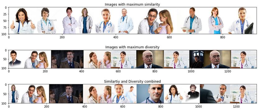
The score avgSim(I) gives us a quantification of how similar the image I is to all other images in
set Tq . Before using this score further, we normalize it by subtracting the mean and dividing by
standard deviation.
                                  \ = avgSim − mean(avgSim) .
                                avgSim
                                                std(avgSim)
    However, we cannot expect the ranking with respect to this measure to be diverse. Using the
second set TF , we construct a diversity score matrix div of size |TF | × |S|, where the element
corresponding to I ∈ S and IF ∈ TF has the value

                                        div(IF , I) := sim(IF , I).

Once again, we normalize each row of the div matrix by subtracting the mean of the row and
dividing by its standard deviation. We call the normalized matrix div.
                                                                     c
    To combine the scores, we construct a diversity-similarity score matrix divSim of size |TF | × |S|,
where the element corresponding to I ∈ S and IF ∈ TF has the value

                        divSim(IF , I) := α · div(I                  \
                                              c F , I) + (1 − α) · avgSim(I),

where α ∈ [0, 1]. Finally, we return the set of images with maximum score in each row of the matrix
divSim (checking for duplicates at each step).

2.1   Obtaining Similarity Scores
To obtain the similarity score sim(I1 , I2 ) for two given images, we can utilize a pre-trained convo-
lutional neural network.
    We use the pre-processed VGG-16 network [25] for generating the feature vectors 1 . VGG-16
is a 16-layer convolutional neural network. We take the weights of the edges after the last fully-
connected layer as the feature vector for the image. The process can be summarized in the following
steps 2 .
   • Feed the image into the VGG-16 network and obtain the feature vector of dimension 4096 as
     described above.
   • Perform Principal Component Analysis to reduce the feature vector size.
   • Compute the cosine distance, D(u, v), between the feature vectors as the similarity score.
     The cosine distance between two vector u, v is defined as
                                                             u·v
                                          D(u, v) = 1 −              .
                                                           kuk2 kvk2

Finally, we return sim(I1 , I2 ) = DvI1 ,vI2 , where vIj is the feature vector corresponding to image Ij .
Remark 2.1 (Other methods). We use other CNN based methods as well, such as retraining part
of a given VGG-16 network using the diversity control set TF . However the results produced were
not as good as the pre-trained network, possibly due to small size of training set TF . Furthermore,
retraining the network, or even a part of it, introduces an overhead computation, while in comparison
the above method uses the CNN as a blackbox. The results for the experiments using a retrained
network are provided in the Appendix C.

                                                    4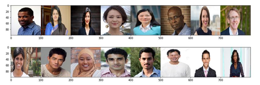
Figure 3: Percentage of women in top 100 results using Algorithm in Section 2.1 for gender pre-
labelled images (α = 0.5) vs Google Image Search results. While the line for Images obtained
using only similarity scores seems balanced, it can be seen that the variance of the points is large.

3        Related Work
The study by [19] explored the effects of bias in image search results of occupations on the perception
of people of that occupation. The major aim of the study was to understand whether the biased
portrayal of minorities in image search results leads to stereotypes or not. Such a phenomenon
has been observed in other forms of media like television [5]. [15] also showed that the annotated
datasets of English and German, used for various NLP tasks and tools, are age-biased. Studies
like these have brought to light the problem of bias in common ML algorithms and led to a surge
of research in fair algorithms. In the field of computer vision, [6] showed that the existing facial
analysis datasets are biased with respect to gender and skin type. Summarization algorithms using
such datasets can lead to biased results and hence a feedback loop . Correspondingly, it becomes
important to develop summarization algorithms that ensure “visible diversity” even when using
biased datasets.
    Current approaches to debias summarization algorithms often assume the existence of sensitive
attribute labels for data-points. For example, [8] formulate the summarization problem as sampling
from a Determinantal Point Process and use partition constraints on the support to ensure fairness.
Setting up the partition constraints requires the knowledge of the partitions and correspondingly
the sensitive attributes for all datapoints. Similarly, fair classification algorithms, such as [7, 9,
11, 13, 18, 26, 27] use the gender labels during the training process, but may or may not use it
once the model is generated. In the context of image-related tasks, [28] looked at the datasets and
models used for language-based image recognition tasks, such as captioning an image, and found
that there exists significant gender bias in the data and models. They suggest constraints based
modifications of existing models to ensure fairness of these models, but the constraints are based
on the knowledge of the gender labels.
    1
        Other networks such as [24] can also be used.
    2
        Similar to github.com/ankonzoid/artificio.

                                                        5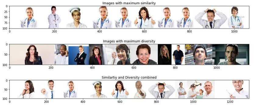
Figure 4: Comparison of accuracy, as measured using mean similarity scores, of top 100 results
across all occupations. For each occupation, we also plot the standard deviation using the dotted
lines.
    There are other works that attempt to ensure diversity in the learning algorithm without using
gender or race labels. [4] consider the problem of gender bias in word embeddings trained on Google
News articles and provide methods to modify the embeddings to debias them. Through standard
gender-related words, they identify the direction of the gender bias in given word embeddings and
then attempt to remove it.
    To identify image similarity, a number of techniques have been explored [16]. The usual tech-
niques before the use of Convolutional Neural Networks included the following: Blob detection
[20], involves finding the part of the image which is consistent across all images, Template match-
ing [17], where we are given a template image against which all other images are to be matched
after pre-processing steps, and SURF feature extractor [3] which detects local feature, generates
their description and then matches these features across images.
    However, the use of convolutional neural networks for image classification has resulted in a vast
improvement in accuracy. In particular, networks like VGG-16 and VGG-19 [25], pre-trained on
datasets like ImageNet [1], can be very easily used for various classification tasks. Hence, it makes
sense to use pre-trained CNNs for the task of image matching.
    This method of using pre-trained models for other tasks is also called “transfer learning”. This
technique has been used in many other classification tasks, such thoraco-abdominal lymph node
detection and interstitial lung disease classification [14], or object and action classification [23], and
has shown significant improvement compared to previous work.

                                                    6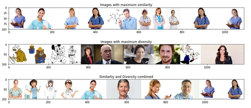
Figure 5: Standard deviation of {N (IF ) | IF ∈ TF } for different occupations, where N (IF ) = |{I |
IF = arg min{sim(I, IF0 ) | IF0 ∈ TF }}|. It basically is the number of images similar to IF in the top
100 results. The lower the standard deviation of this quantity, the more diverse is the set.

4        Experiments
4.1       Dataset
The dataset used in the experiments is the same as the one in the paper Kay, Matuszek and Munson
[19]. The dataset includes top Google Image Search results for 96 different occupations 3 . The total
number of images is around 38400 and the average number of images per occupation is 400.
    For each occupation, we use the top 10 images as the similarity control set Tq , to be used
to match similarity against if that particular occupation is queried. Similarly, we construct a
diversity control TF using visibly diverse images. The set TF used in the experiments is provided
in Appendix D.
    We use a visibly diverse control set of images but other methods of choosing a diverse set (such
as images from all classes of Fitzpatrick skin-types [12]) can also be considered.
    A subset of the images (around 10%) is also gender-labelled using feedback from Mechanical
Turk. On an average, 72 images from each occupation are gender-labelled and the images labelled
are “clear”, i.e., they have a single person in the image and the features of the person are clearly
visible. We use this subset and other methods to calculate the diversity of our results.
    Note that this dataset is of Google Image results from 2015 and we use it due to existing
analysis on the occupations and gender information of the images in the dataset, as provided by
[19]. However any other image dataset can also be used in the place of this dataset and the
algorithms remains the same.
    3
        https://github.com/mjskay/gender-in-image-search

                                                     7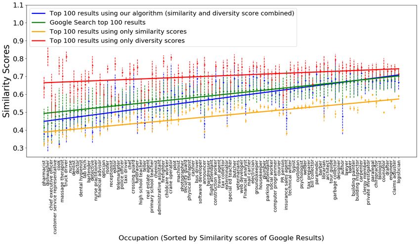
(a) CEOs                                        (b) Doctors

Figure 6: Top images returned by the algorithm when the dataset is restricted to the queried
occupation. The results show that even when accuracy is guaranteed the returned images are
visibly diverse.

Remark 4.1. For the images without gender labels, we attempt to use pre-trained gender classifica-
tion tools [21] to auto-label the gender of the images, so as to better evaluate the performance of our
algorithm. However such tools might themselves be biased due to biased training data or algorithms,
and therefore we focus more on the diversity results obtained using the gender pre-labelled images
or visible diversity. The results corresponding to images with auto-labelled gender are presented in
Appendix B.

4.2     Results using Pre-Trained VGG-16
For the results below, we use the neural-network based method, described in Section 2.1. We also
vary α and look at its impact on the accuracy of the results (A preliminary analysis is presented
in Appendix A).
    Figures 2 present a few examples corresponding to the output for different occupation queries.
As it can be seen from the figures, after combining the similarity and diversity scores, the top
images obtained are visibly diverse.
    When the dataset is restricted to images with pre-labelled gender, the gender diversity of our
results compared to the gender diversity of Google image results can be seen in Figure 3. The
x-axis in this plot is the actual percentage of women in occupations, the data for which is provided
by the US Bureau of Labor and Statistics [2]. While the percentage of women in Google image
results varies quite drastically across occupations, our image results are much more balanced.
    Furthermore for Google Image search, the average fraction of women in top 100 results of any
occupation is 0.37 with a standard deviation of 0.32, while for our algorithm, the average fraction
of women in top 100 results of any occupation is 0.54 with a standard deviation of 0.13, which is
much more balanced. When using only similarity score, the average fraction is 0.44 with a standard
deviation of 0.26 (which is why the line for algorithm with only similarity score in Figure 3 is slightly
misleading due to the high variance) and when using only diversity score, the average fraction is
0.51 with standard deviation 0.
    We provide further empirical evidence of the accuracy and diversity of the output images in
this section.
4.2.1    Accuracy
Since its important to first check how accurate our method is in finding similar images, we present
accuracy results for the same below.

                                                   8
Figure 7: Comparison of racial diversity of the top images from our algorithm, Google Image Search
and the baseline algorithms
Correspondingly, we compare our accuracy with Google Image results. For each occupation,
given the top 100 results from each method, we again compute the avgSim score for each image
in the set. Then, we compute the mean and standard deviation of this score and plot it for each
occupation in Figure 4. The plot also has the similarity scores for baseline results, such as the
results returned when we rank by only similarity scores or by only diversity scores.
From the figure, we can see that the average similarity score of the top 100 images of our
algorithm is similar to the top 100 images of Google image search. For the baselines, as expected,
the algorithm using only similarity scores has the best accuracy and the algorithm using only
diversity scores has the worst. For some occupations however, the Google result score is higher than
our score. Upon checking the returned images from these occupations, we found that there were two
reasons for this. For certain occupations, like pharmacist, our top results include those of doctors
as well, whereas Google’s results are more accurate. On the other hand, for some occupations
like librarian, our top results were of people in library while Google’s top results included a lot of
cartoons images.
We plot the bar graph showing the number of results of the given occupation in top 100 images
when that occupation was queried in Figure 8. However since images of multiple professions might
be similar (like CEOs, financial analysts and lawyers), for each query occupation we also present
the other occupation with the most results in top 100 images. While for a significant fraction of
occupations the percentage of images in top 100 results belongs to the same class is greater than
40%, from Figure 8, it is still difficult to judge from the bar graph itself whether the method is
accurate or not, and so Figure 4 is a better measure of judging accuracy.
Overall, we can conclude that the top images returned are visually similar to the queried images
and that our method is matches the Google’s results in terms of accuracy.
9Figure 8: Bar chart with number of results of the queried occupation in top 100 results for each
occupation when the algorithm uses pre-trained VGG-16 network and then computes similarity
scores. α = 0.3.
4.2.2 Diversity using gender pre-labelled images
Using the gender pre-labelled set of images as the total set S, we look at the percentage of women in
the top 100 results for a given query occupation. We compare this against the percentage of women
in the top 100 results of Google Image Search in Figure 3, the data for which is also provided by
[19] for certain filtered occupations. The figure shows the images obtained using our algorithm are
much more gender-balanced than Google Search Image results for the same queries.
4.2.3 Visible Diversity
It is important to ensure that the top images returned by the algorithm are visibly diverse even
when the accuracy is ensured to be high. To check visible diversity, we restrict our dataset to a
single occupation (ensuring accuracy) and check if the returned images are visibly diverse. For
datasets restricted to only CEOs and only Doctors, the top images returned by the algorithm are
presented in Figure 6.
4.2.4 Diversity Comparison
Since only a small percentage of the dataset has gender labels, we need other metrics to ensure that
the images returned by our algorithm are indeed diverse. A good measure of diversity is, given the
top 100 results from our algorithm, the number of images in this set similar to a particular image
in the diversity control set TF is almost the same for all images in TF . We use this idea to compare
the diversity of our results on the full dataset to the Google Image search results.
We are given the top 100 results of our algorithm on the full dataset and the top 100 results
from Google Search. Let
minDivScore(I) := min{sim(I, IF ) | IF ∈ TF }.
10We calculate the score list minDivScore for the given set T and for each image I ∈ T , we also store
the image in TF for which it achieves the score minDivScore(I), i.e.,
arg min{sim(I, IF ) | IF ∈ TF }.
Then for each image IF ∈ TF , we calculate the number of images in T most similar to it, i.e., the
number of images I ∈ T for which minDivScore(I) = sim(IF , I). Lets call this number N (IF ).
Formally,
N (IF ) = |{I | IF = arg min{sim(I, IF0 ) | IF0 ∈ TF }}|.
For each occupation, we calculate the standard deviation of {N (IF ) | IF ∈ TF } and plot it in
Figure 5. Once again, the idea is that if the returned set of images is diverse, then the standard
deviation of the above list should be small, since the similarity of images should be equally dis-
tributed across all images in TF . From the figure, it can be seen that the images returned by our
algorithm on the full dataset has lower standard deviation than Google Image results. We also plot
the standard deviation of {N (IF ) | IF ∈ TF } for baseline algorithms that use only similarity scores
or only diversity scores for reference.
4.2.5 Diversity with respect to Race
We inspect the racial diversity of the top results of our algorithm and compare it to the diversity
of the top results of Google Image Search and the baseline algorithms. Since the race of the people
in the images is not pre-labelled, we do this analysis for only a small percentage of the top results.
In particular, we look at the top 16 images from each algorithm (we choose 16 because that is the
size of the diversity control set TF 14. We also look at only those occupations for which the top
16 Google images are mostly of people, and not cartoons or objects. The results are presented in
Figure 7.
From the figure, one can see that all our algorithm is much more balanced in terms of percentage
of minorities in top results than Google search, which as expected performs similar to the algorithm
using only similarity scores. However, even though our algorithm is relatively better, the figure
shows all the algorithms are still quite unbalanced. A better choice of the diversity control set and
a more robust dataset can lead to better results.
5 Limitations and Future Work
The algorithm and results presented here is a prototype that aims to use existing methods to
improve diversity in image summarization. However, there are certain limitations to this approach
which we examine in connection to potential future work in this section.
First and foremost, it is important to state that our primary evaluation of our method was with
respect to gender. This evaluation made use of pre-labelled data which treated gender as binary,
which is unnecessarily and problematically restrictive and not an accurate representation of the
gender diversity in humanity. The problem with binary gender-labelling is a severe limitation in
all works on fairness and has been expressed in papers like [12] as well. It would be important to
consider evaluate this work in light of other datasets, sensitive attributes, and broader label classes.
One challenge of using this approach is that it may not always be easy to evaluate its success.
Its main strength – that it can diversify without needing class labels in the training data – is also
an important weakness because we may not have labeled data with which to evaluate the results.
One approach would be to use predict labels using, e.g., gender classification tools [21]; we present
the results for such an approach in a larger image dataset in Appendix B. However, we do not
11recommend using predicted labels in general as such classification tools can themselves introduce
biases and are currently not designed with broader label classes in mind, and hence do not address
the core problem. Perhaps a better approach would be to use human evaluators do rate or define
the visible diversity of the images selected by the algorithm.
An important consideration in using this approach is in the construction of the diversity control
set (the one that we use is presented in full in Appendix D). The goal would be to have any such
set be visibly diverse with respect to attributes such as gender, ethnicity, or country of origin.
However, the exact set to be used (and/or the exact demographics desired) may differ depending
on the application, and the set must be constructed in a thoughtful and context-aware manner.
Perhaps more scientifically accurate methods of constructing diverse control sets can be employed,
for example by taking images from across the Fitzpatrick skin-type scale [12].
The algorithm to obtain similarity scores can be improved a lot given other information about
the source of the image. For example, for a model similar to Google Image search, one would
have access to the metadata of the image which will help better judge the similarity of two pages.
With such additional information, we expect our algorithm to perform much more accurately.
Other transfer learning techniques, like retraining a small part or a single layer of the CNN, could
potentially be employed for better feature extraction, although we did not see any improvement on
an initial approach in this direction (see Appendix C).
6 Conclusion
To the best of our knowledge, this is the first approach to fairness in any application area that does
not require (implicitly or explicitly) labeled data in order to ensure diversity. As a post-processing
approach, it is also incredibly flexible in that it can be applied post-hoc to an existing system
where the only additional input necessary is a small set of “diverse” images. We show its efficacy
on an image dataset of occupations and show that it can significantly improve the diversity of the
images selected with little cost to accuracy as compared to images selected by Google. Due to the
generality and simplicity of the approach, we expect our algorithm to perform well for a variety of
domains, and it would be interesting to see to what extent it can be applied in areas beyond image
summarization.
References
[1] Image-net. http://www.image-net.org/.
[2] Bureau of labor statistics. labor force statistics from the current population survey. https:
//www.bls.gov/cps/aa2012/cpsaat11.htm, 2013.
[3] Herbert Bay, Tinne Tuytelaars, and Luc Van Gool. Surf: Speeded up robust features. In
European conference on computer vision, pages 404–417. Springer, 2006.
[4] Tolga Bolukbasi, Kai-Wei Chang, James Y Zou, Venkatesh Saligrama, and Adam T Kalai.
Man is to computer programmer as woman is to homemaker? debiasing word embeddings. In
Advances in Neural Information Processing Systems, pages 4349–4357, 2016.
[5] Sherryl Browne Graves. Television and prejudice reduction: When does television as a vicarious
experience make a difference? Journal of Social Issues, 55(4):707–727, 1999.
12[6] Joy Buolamwini and Timnit Gebru. Gender shades: Intersectional accuracy disparities in
commercial gender classification. In Conference on Fairness, Accountability and Transparency,
pages 77–91, 2018.
[7] L Elisa Celis, Lingxiao Huang, Vijay Keswani, and Nisheeth K Vishnoi. Classification
with fairness constraints: A meta-algorithm with provable guarantees. arXiv preprint
arXiv:1806.06055, 2018.
[8] L Elisa Celis, Vijay Keswani, Damian Straszak, Amit Deshpande, Tarun Kathuria, and
Nisheeth K Vishnoi. Fair and diverse dpp-based data summarization. arXiv preprint
arXiv:1802.04023, 2018.
[9] Sam Corbett-Davies, Emma Pierson, Avi Feller, Sharad Goel, and Aziz Huq. Algorithmic de-
cision making and the cost of fairness. In Proceedings of the 23rd ACM SIGKDD International
Conference on Knowledge Discovery and Data Mining, pages 797–806. ACM, 2017.
[10] Amit Datta, Michael Carl Tschantz, and Anupam Datta. Automated experiments on ad
privacy settings. Proceedings on Privacy Enhancing Technologies, 2015(1):92–112, 2015.
[11] Cynthia Dwork, Moritz Hardt, Toniann Pitassi, Omer Reingold, and Richard Zemel. Fairness
through awareness. In Proceedings of the 3rd innovations in theoretical computer science
conference, pages 214–226. ACM, 2012.
[12] Thomas B Fitzpatrick. The validity and practicality of sun-reactive skin types i through vi.
Archives of dermatology, 124(6):869–871, 1988.
[13] Moritz Hardt, Eric Price, Nati Srebro, et al. Equality of opportunity in supervised learning.
In Advances in neural information processing systems, pages 3315–3323, 2016.
[14] Shin Hoo-Chang, Holger R Roth, Mingchen Gao, Le Lu, Ziyue Xu, Isabella Nogues, Jian-
hua Yao, Daniel Mollura, and Ronald M Summers. Deep convolutional neural networks for
computer-aided detection: Cnn architectures, dataset characteristics and transfer learning.
IEEE transactions on medical imaging, 35(5):1285, 2016.
[15] Dirk Hovy and Anders Søgaard. Tagging performance correlates with author age. In Proceed-
ings of the 53rd Annual Meeting of the Association for Computational Linguistics and the 7th
International Joint Conference on Natural Language Processing (Volume 2: Short Papers),
volume 2, pages 483–488, 2015.
[16] N Jayanthi and S Indu. Comparison of image matching technique. J. Latest Trends Eng.
Technol, 7:396–401, 2016.
[17] Di Jia, Jun Cao, Wei-dong Song, Xiao-liang Tang, and Hong Zhu. Colour fast (cfast) match:
fast affine template matching for colour images. Electronics Letters, 52(14):1220–1221, 2016.
[18] Faisal Kamiran and Toon Calders. Data preprocessing techniques for classification without
discrimination. Knowledge and Information Systems, 33(1):1–33, 2012.
[19] Matthew Kay, Cynthia Matuszek, and Sean A Munson. Unequal representation and gender
stereotypes in image search results for occupations. In Proceedings of the 33rd Annual ACM
Conference on Human Factors in Computing Systems, pages 3819–3828. ACM, 2015.
13[20] Hui Kong, Hatice Cinar Akakin, and Sanjay E Sarma. A generalized laplacian of gaussian filter
for blob detection and its applications. IEEE transactions on cybernetics, 43(6):1719–1733,
2013.
[21] Gil Levi and Tal Hassner. Emotion recognition in the wild via convolutional neural networks
and mapped binary patterns. In Proceedings of the 2015 ACM on international conference on
multimodal interaction, pages 503–510. ACM, 2015.
[22] Kristian Lum and William Isaac. To predict and serve? Significance, 13(5):14–19, 2016.
[23] Maxime Oquab, Leon Bottou, Ivan Laptev, and Josef Sivic. Learning and transferring mid-
level image representations using convolutional neural networks. In Proceedings of the IEEE
conference on computer vision and pattern recognition, pages 1717–1724, 2014.
[24] Florian Schroff, Dmitry Kalenichenko, and James Philbin. Facenet: A unified embedding for
face recognition and clustering. In Proceedings of the IEEE conference on computer vision and
pattern recognition, pages 815–823, 2015.
[25] Karen Simonyan and Andrew Zisserman. Very deep convolutional networks for large-scale
image recognition. arXiv preprint arXiv:1409.1556, 2014.
[26] Muhammad Bilal Zafar, Isabel Valera, Manuel Gomez Rodriguez, and Krishna P Gummadi.
Fairness constraints: Mechanisms for fair classification. arXiv preprint arXiv:1507.05259, 2015.
[27] Brian Hu Zhang, Blake Lemoine, and Margaret Mitchell. Mitigating unwanted biases with
adversarial learning. arXiv preprint arXiv:1801.07593, 2018.
[28] Jieyu Zhao, Tianlu Wang, Mark Yatskar, Vicente Ordonez, and Kai-Wei Chang. Men also like
shopping: Reducing gender bias amplification using corpus-level constraints. arXiv preprint
arXiv:1707.09457, 2017.
14Figure 9: Mean Accuracy (with standard deviation on error bars) of the search results vs α value.
A Impact of α on Accuracy
We also look at the impact of varying the parameter α on the mean accuracy of the search results.
Here we measure the accuracy as the number of images in top 100 with the same occupation as
the query occupation. The choice of α represents the balance between accuracy and diversity. The
affect of change of α on accuracy is shown in Figure 9. Hence we use α ∈ [0.3, 0.5].
B Diversity using gender auto-labelled images
Since a very small subset of total number of images had gender labels (around 10%), we use certain
gender detection tools to auto-detect the gender of the person in the image. In particular, we use
the work of Levi and Hassner [21] to automatically detect gender of the image. The code for the
same is available at https://github.com/dpressel/rude-carnie.
It is important to note that in general, we can expect that such auto-labelling tools also suffer
from bias resulting from possible biased training data. Also we do not labels for which the confidence
of the algorithm is lower than a certain threshold.
Using the gender labels from the detection tool, we calculate the percentage of women in the
top 100 images from our algorithm against the percentage of women in the top 100 results of
Google Image Search in Figure A, the data for which is also provided by [19] for certain filtered
occupations.
C Results using Re-trained VGG network
The method used here is modification of the one in Section 2.1. In this method, we attempt to
modify the pre-trained CNN to ensure diversity.
15Figure 10: Accuracy graph when the algorithm uses re-trained VGG-16 network.
b
Figure 11: Percentage of women in top 100 results using our algorithm for gender auto-labelled
images vs Google Image Search results.
16Figure 12: Percentage of women in top 100 results using our algorithm with retrained network for
different occupations.
• Re-train the last fully-connected layer of VGG-16 using the diverse control set TF .
• Feed the images from S into the re-trained VGG-16 network and obtain the feature vector of
dimension 4096 as described above.
• Compute the cosine distance between the feature vectors as the similarity score.
Note that using this method, we do not need to maintain any diversity-similarity score matrix,
since the diversity is expected to be ensured by the CNN itself.
C.1 Accuracy
We first check how accurate our method is in finding similar images. Figure 10 presents a bar
graph showing the number of results of the given occupation in top 100 images returned when that
occupation was queried. Here again for each query occupation we also present the other occupation
with the most results in top 100 images. Note that for most occupations, the top two combined
result in more than 50% of the top 100 images.
C.2 Diversity
Once again using the gender pre-labelled set of images as the total set S, we look at the percentage
of women in the top 100 results for a given query occupation. The result for different occupations
are presented in Figure 12.
We also compare this against the percentage of women in the top 100 results of Google Image
Search in Figure 13(a). The figure shows the images obtained using our algorithm are much more
gender-balanced than Google Search Image results for the same queries and even more balanced
than the earlier method.
C.3 Diversity using gender auto-labelled images
Once again, we also present the results abotained using the gender labels from the detection tool
[21]. We calculate the percentage of women in the top 100 images from our algorithm against the
percentage of women in the top 100 results of Google Image Search in Figure 13(b).
17(a) Gender pre-labelled (b) Gender auto-labelled
Figure 13: Percentage of women in top 100 results using Algorithm in Section C for gender
auto-labelled images and gender pre-labelled images vs Google Image Search results.
D Diversity Control Set
The diversity control set used in the main experiments is given in Figure 14.
E Diversification Across Other Image Types
In addition to sensitive attributes like gender, this approach can induce diversity with respect to
other features as well. In this section, we examine this approach by considering a diversity control
set of equal number of cartoon and non-cartoon images. Detecting whether an image is a cartoon
or not is relatively easier than other attributes like the gender or race of the image, since a cartoon
Figure 14: Diversity Control Set used in the images.
18(a) Nurse (b) Typist
Figure 15: Top images returned by the algorithm when the diversity control set TF contains equal
number of cartoon and non-cartoon images.
image has less “number” of colors than a image of a real person. The rest of the implementation
details are the same as the previous section.
E.1 Results
The resulting images for cartoon based diversification for a few example occupation can be seen in
Figure 15. As we can see, the cartoon images chosen in the top results correspond or are related
to the query occupation.
E.2 Accuracy
Once again, we make a bar graph of the accuracy for each occupation, presented in Figure 16. In
this case the accuracy lower than before, since for most queried occupations, there are few cartoon
images corresponding to that occupation.
E.3 Diversity
To check diversity, we compare the top 100 results of our algorithm to the top 100 results obtained
when using only similarity scores. The results are presented in Figure 17 As expected, when using
only similarity scores, the number of cartoon images in the top 100 would be very skewed. On the
other hand, our algorithm, with similarity and diversity scores combined, will have a more balanced
ratio of cartoon and non-cartoon images.
19Figure 16: Accuracy chart of top 100 results for each occupation when the diversity control set has
equal number of cartoon and non-cartoon images. α = 0.4.
Figure 17: Comparison of cartoon diversity of our algorithm vs Google results and baseline algo-
rithms.
20You can also read