INCOME CHANGES AND CONSUMPTION: EVIDENCE FROM THE 2013 FEDERAL GOVERNMENT SHUTDOWN
←
→
Page content transcription
If your browser does not render page correctly, please read the page content below
INCOME CHANGES AND CONSUMPTION:
               EVIDENCE FROM THE 2013 FEDERAL
                          GOVERNMENT SHUTDOWN ∗

                             Scott R. Baker†                  Constantine Yannelis‡

                                                     May 2015

                                                        Abstract

         We use the 2013 federal government shutdown and a rich data set from an online personal finance
         website to study the effects of changes in income on changes in consumption. The 2013 shutdown
         represented a significant and unanticipated income shock for federal government workers, with no di-
         rect effect on permanent income. We exploit both the differences between unaffected state government
         employees and affected federal employees as well as between federal employees required to remain
         at work and those required to stay at home to generate variation in income and leisure time. We find
         strong evidence for excess sensitivity of consumption patterns, violating the permanent income hy-
         pothesis. We demonstrate that this decline in spending can be largely explained by increased home
         production, changes in spending allocations, and credit constraints. We are able to discern detailed cat-
         egories of household spending with widely varying elasticities. The results demonstrate the importance
         of household liquidity, leisure, and home production when constructing stimulus or social insurance
         policy.
         JEL Classification: D10, E20, E64, H31

   ∗
       The authors wish to thank Nick Bloom, Caroline Hoxby, Adam Isen, Adam Looney, Petra Persson, Nick Turner
and Luigi Pistaferri for helpful comments and suggestions, as well as seminar and conference participants at the
All California Labor Conference at UC Berkeley, the Consumer Financial Protection Bureau Research Conference,
Kellogg School of Management, and Stanford University. The authors thank Kellogg School of Management, Donald
P. Jacobs, the Alexander S. Onassis Foundation, SIEPR and the Kapnick Foundation for funding and support.
    †
      Dept of Finance, Kellogg School of Management, Evanston, IL 60208. s-baker@kellogg.northwestern.edu
    ‡
      Dept of Economics, Stanford University, 579 Serra Mall, Stanford, CA 94305. yannelis@stanford.edu

                                                            1
1    Introduction
There is a substantial body of work documenting the excess sensitivity of changes in consumption
to changes in income. However, observed changes in consumption can be due either to changes in
beliefs about permanent income, liquidity issues, or to factors related to changes in time allocation
such as the non-separability of leisure and consumption in the utility function, or home production.
Drops in consumption due to changes in time allocation have very different welfare implications
than drops in consumption due to shifts in permanent income or credit constraints, impacting
the optimal construction of government insurance programs such as unemployment insurance and
social security.
    This paper uses the 2013 federal government shutdown as a natural experiment to examine the
effect of changes in income and time allocation on consumption. We make two main contributions.
First, we provide evidence of excess sensitivity of consumption to temporary changes in income
with no change in permanent income or wealth. The fact that nominal permanent income would not
change was known from the early days of the shutdown. Second, we exploit institutional specifics
of the shutdown to show that changes in the time allocation of workers lead to large effects on
consumption patterns. Up to half of the decline in spending is due to changes in time allocation
and work-related expenses.
    The link between income and consumption is one of the most researched relationships in eco-
nomics. However, when attempting to apply some of the workhorse consumption models to the
data, difficulties often arise. Speaking about violations of the permanent income model in their
survey paper, Jappelli and Pistaferri (2010) note that:

      ...One encounters two types of problems when trying to provide a clean test of the [permanent in-
      come] theory: one empirical and one theoretical. On the empirical side, it is difficult to identify sit-
      uations in which income changes in a predictable way. But even if the empirical problems can be
      surmounted, there are many plausible explanations why the implications of the theoretical models may
      be rejected, ranging from binding liquidity constraints to non-separabilities between consumption and
      leisure, home-production considerations, habit persistence, aggregation bias, and durability of goods.

    This paper leverages highly-detailed household level data to more comprehensively explore
the relationship between temporary income shocks and consumption. In the context of the US
federal government shutdown of 2013, we are able to isolate a purely temporary income shock,

                                                         2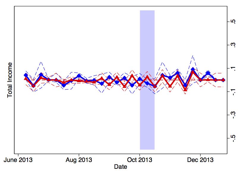
wherein the sole effect is that income is reallocated from one paycheck to the next, two weeks
later. Importantly, this paper is the first, to our knowledge, to be able to jointly examine the
role that home production, credit and liquidity constraints, and substitution between categories of
spending play in driving consumption responses to a temporary income shock.
    Looking narrowly, this paper can help to understand how, conditional on permanent income
being unaffected, both the level and composition of household spending change significantly dur-
ing non-employment spells.1 More broadly, this paper contributes to a growing literature about
heterogeneous household consumption behavior and the importance of considering liquidity and
credit in structural models.
    Overall, this paper demonstrates three primary facts. The first is that, relative to the canonical
permanent income model, we find striking evidence of excess sensitivity of household spending
due to a purely temporary income shock. Second, we demonstrate that households are quick to
reallocate spending across both time and categories of consumption. For most households seeing
spending declines, much of the foregone spending is ‘made up’ following the repayment of their
lost wages. Moreover, home production is an important channel through which households adjust
the composition of their spending during the shutdown. Finally, this paper contributes to recent
work suggesting that even relatively high-income households are impacted by temporary income
declines due to hand-to-mouth spending, and we present evidence that a large driver of the observed
excess sensitivity is liquidity and credit constraints.
    This paper is organized as follows. The remainder of this section discusses the 2013 US federal
government shutdown, which is used to identify the excess sensitivity of consumption to changes
in income and decompose the effect into time allocation and income related components. Section
2 discusses the data derived from a large personal online finance platform. Section 3 discusses our
empirical strategy and potential drivers of the observed effects. Section 4 details our results, while
section 5 concludes.
   1
     This includes changes in the composition during periods of unemployment as well as following retirement or
periods outside the labor force.

                                                      3
1.1      The 2013 US Government Shutdown

At the beginning of the 2013 fiscal year, and following the inability of politicians to agree on a
spending plan that included funding for the Patient Protection and Affordable Care Act, the US
federal government ceased most non-essential operations. This shutdown lasted between October
1st and 16th, representing the second longest shutdown since 1980 and the largest measured by
employee furlough days. Table 1 provides an overview of the events leading up to and during the
shutdown, and Burwell (2013) provides an official overview of the impact of the shutdown. During
the shutdown, the majority of civilian federal government employees were not paid.2 Following
the conclusion of the shutdown, employees received all of their foregone pay, totaling approxi-
mately $2 billion. Most federal government workers received their back-pay either in the second
pay period at the end of October, between October 22 and November 1 or during the final months
of 2013. Thus, the operational effect for most affected employees was a cut in pay of approxi-
mately 40% during the first pay period in October and then an increase in pay of approximately
40% during the second pay period in October.3 There was no change in permanent income, only a
temporary income reallocation during the month of October in 2013 for affected federal employ-
ees.
       Workers who were affected by the shutdown (in terms of cuts in pay) were divided into two
groups. ‘Exempted’ employees were required to work without pay during the shutdown, as the
nature of their work was deemed essential to national security, public health or safety. Other
workers deemed non-essential were furloughed and were kept off the job while the shutdown was
in effect. Both groups experienced only a temporary income shock as they were given all of
their foregone earnings following the conclusion of the shutdown. There was significant between-
agency variation in the fraction of employees who were furloughed. For example, employees at the
Departments of Veteran Affairs, Justice and Homeland Security were deemed essential to national
security, and more than three quarters were exempted. During the same time period, approximately
   2
      Some agencies such as the US Postal Service, Federal Courts, the State Department, and uniformed military
personnel are primarily self-funded or funded through special appropriations bills that are not part of the normal
budgetary process. Employees of these agencies were unaffected by the shutdown and were paid during the shutdown.
    3
      The first payday in October was October 11th for most federal employees, covering the dates of September 22nd
to October 5th. Affected employees received checks on October 11th that paid them for work done in September but
not for any work done on or after October 1st. For full time employees, this would represent pay for 6 days of work
rather than the usual 10 days.

                                                        4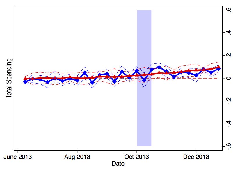
95% of employees at the Department of Education, Department of Housing and Urban Develop-
ment, the Environmental Protection Agency, and the Securities and Exchange Commission were
deemed non-essential and furloughed. For a list of agencies affected by the shutdown see Table 2.
       Thus, we observe ‘unaffected’ workers, who worked at an unaffected federal agency (eg. active
duty military) or a state government agency and are used as controls in this paper. We also observe
‘exempted’ workers, who were unpaid during the shutdown but had to continue working every
day. Finally, we observe ‘furloughed’ workers, who were both unpaid during the shutdown and
were required to stay at home. Both ‘exempted’ and ‘furloughed’ workers were repaid all of their
foregone wages soon after the shutdown’s conclusion.
       The between-agency variation in furloughs is one reason for a wedge in household spending
responses to the temporary income declines. While exempted workers were required to continue
working, furloughed workers were able to forgo work-related expenses like commuting and could
increase home production activities like cooking or performing their own housework. Much work
has focused on this area, finding significant declines in actual expenditures among the unemployed
and retirees but smaller declines in proxies for consumption or utility.4
       The 2013 government shutdown, combined with detailed household financial data, provides a
number of key advantages for studying the effects of changes in income on consumption.5 First,
the shutdown had no effect on permanent income, meaning that the canonical permanent income
hypothesis predicts a precise null hypothesis of zero effect on household consumption. Second,
differences in exempted and furloughed workers allow us to separately examine the home produc-
tion and leisure margins. Finally, data regarding the possession and opening of financial accounts
gives us some ability to measure to what degree credit and liquidity constraints drove the observed
consumption effects.
   4
      A number of authors investigate this point. See Haider and Stephens (2007), Blundell and Tanner (1998), Hurd
and Rohwedder (2006), and Aguiar and Hurst (2007) for a discussion of retirement and home production. Gruber
(1997) and Guler and Taskin (2013) study home production and unemployment spells.
    5
      A subset of results from this paper were discussed in a policy brief Baker and Yannelis (2014). In a paper written
concurrently with this one, Gelman, Kariv, Shapiro, Silverman, and Tadelis (2015) study the effect of the shutdown
on consumption and credit. Their paper focuses on the consumption and credit response to a temporary income drop,
while ours highlights the consumption response to both a temporary income drop and incorporates changes in time
allocation and home production.

                                                           5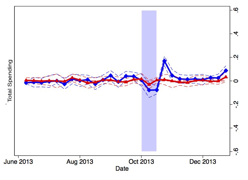
1.2   Mechanics of Delayed Pay

Federal employees were affected to varying degrees by the government shutdown due to differ-
ent pay period calendars at government agencies. For instance, many employees received pay at
monthly increments, meaning their pay generally came at the start or end of each month. This pay
would be unaffected by the government shutdown because by the time their payday for October
arrived (either on the 31st of October or the 1st of November), the shutdown had ended and they
were able to receive their full pay. In this paper, we count these employees as being unaffected by
the shutdown.
    Many other federal employees are on pay period calendars that had them receive bi-weekly
checks on October 11th and 25th. These pay periods covered September 22nd-October 5th and
October 6th-October 19th. The first of these paychecks would see an approximate decline in pay
of about 40% (they received pay only for the 6 days worked in September and none of the days
worked in October). For the paycheck on the 25th, with the shutdown ended, employees would
receive their normal paycheck as well as back pay for the workdays missing from their previous
paycheck. The end result in this example would be 40% lower pay for their first paycheck of
October and 40% higher pay on their second October paycheck. Other variations of this pattern
occurred for employees across differing pay period calendars, but few employees missed an entire
paycheck due to how pay periods lined up with the shutdown.

2     Data
The data used in this paper comes from a large online personal finance website. The site provides
a service that connects users’ financial accounts so that the user can see all of their accounts in a
single location. The site allows for users to easily see summaries of their income, spending, debt,
and investments across all of their accounts and has other features such as budgeting or financial
goal-setting. The site has grown rapidly, from under 300,000 users in 2007 to more than 3 million
active users by 2013. This large userbase has yielded a database of more than 5 billion transactions
across over 10 million individual accounts. These accounts span all manner of household financial
products including checking accounts, savings accounts, credit cards, loans, property and mortgage

                                                 6
accounts, equity portfolios, and retirement accounts.6
       The data are automatically linked from financial accounts to the website, allowing for less mea-
surement error and potential recollection biases relative to other survey-based household financial
data. In this paper, we focus primarily on two aspects of the data. The first is on paycheck income
derived from government employers. To identify users with relevant employers, we take a simi-
lar approach as in Baker (2014), but focus on state and federal government agencies rather than
publicly-traded companies. We match users to their employers using textual descriptions from
users’ direct deposit transactions. Direct deposit transfers into checking accounts are generally ob-
served with little error, allowing us to focus on these paycheck deposits and exclude other sources
of income. Direct deposit transaction descriptions are generally characterized by indicators that the
transaction is a direct deposit, a string representing an employer or agency, and anonymized iden-
tifiers.7 Our strategy for matching allows us to ignore punctuation and limited misspellings and is
mainly drawn from the inspection and testing of several million paycheck transaction descriptions.
       Our paycheck matching strategy yields a set of 152,810 households. 91,650 of these are em-
ployed by 52 unaffected federal agencies and state governments to be used as the control group
during and surrounding the shutdown period. 61,160 users are able to be matched to 19 different
federal agencies including NASA, the Securities and Exchange Commission, the Senate and House
of Representatives, and a range of federal departments such as Labor, the Interior, Transportation,
and State. We restrict to a balanced panel of users present in the data from January 2013 to De-
cember 2013. Given the strategy we employ, there is unlikely to be measurement error in agency-
employee matching at the individual user level. This is due to the fact that a given government
agency or department has a near uniform description attached to its direct deposit transactions.
Thus, an error in matching would likely miss an entire class of employees or be unable to match
any employee from a given agency rather than having only some employees matched while others
are unmatched. One important caveat is that the paycheck transactions that we observe are net of
any taxes or benefits withheld from employee paychecks. Thus, we cannot directly observe 401k
contributions, federal and state taxes, or healthcare premiums paid out of gross pay.
   6
     For the purposes of this paper, account balances are unable to be observed at a household level. Our analysis
examines flows, such as income and spending, and the presence and change in number and types of financial accounts.
   7
     Some examples of such descriptions are: “DEPT JUSTICE DIRECT DEP XLWK”, “PAYROLL DEPOSIT
HHS”, and “TRANSIDRRRR81 STATE TENNESSDIR”

                                                        7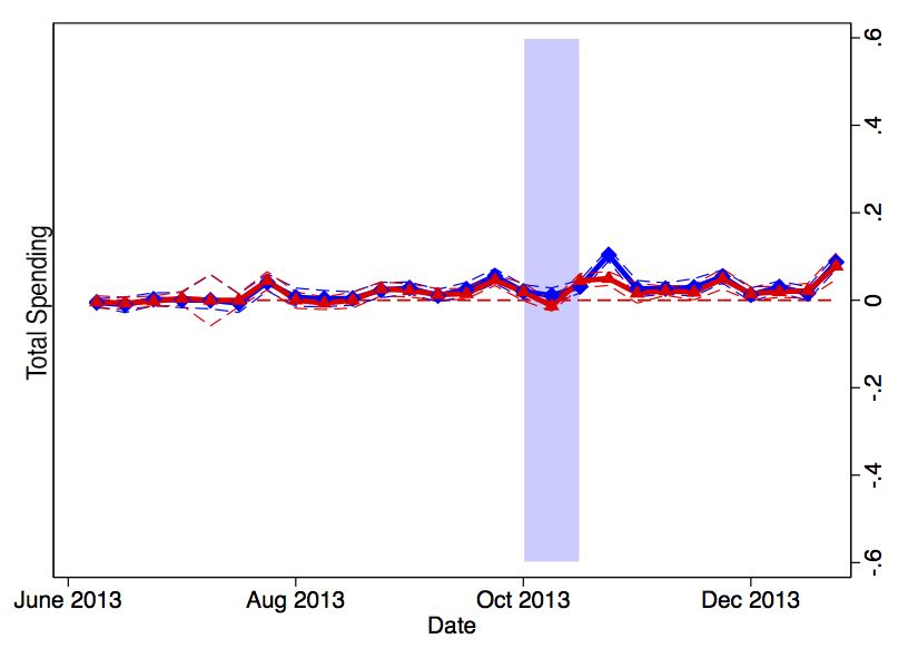
In addition, using data from the OMB’s list of federal agency contingency plans, we note the
fraction of the employees at each agency or department that were affected by the government shut-
down.8 The fractions of employees affected ranged from 26% or less at the Department of Veterans
Affairs, Customs and Border Patrol, the Department of Justice, and Department of Transportation
to more than 85% at the IRS, NASA, EPA, Department of Education, and Department of Com-
merce. In addition, a number of agencies, including the federal court system and Supreme Court,
active duty military members, the US Post Office, and the FDA were unaffected by the shutdown
due to exemption or other sources of funding.
       Our second focus is on transactional spending data derived from bank, debit, and credit card
transactions. These data offer a rich view of spending by users and comprise the vast majority of
total household spending among users. Each transaction is time-stamped, has a full description and
is generally also matched to information about the merchant. From this merchant and descriptive
data, the site automatically categorizes each transaction into one of over 100 categories (such as
‘Groceries’, ‘Gasoline’, ‘Student Loans’, ‘Fast Food’, or ‘Mortgage Payment’) in order to provide
easily readable spending and income breakdowns to the user. From these data, we can derive mea-
sures of total household spending across all categories as well as subsets of spending based on the
categorization of the transactions. One potential omission is that of cash transactions. Cash trans-
actions can only be fully observed when a user manually enters them, though strong assumptions
about cash spending can also be made by observing ATM and bank withdrawals. An estimated
8-9% of total spending is done with cash in the United States, compared to approximately 3-4% of
spending done with cash in the sample data.9
       These data are described in more detail in Baker (2014), along with a number of ancillary tests
and descriptive statistics. Steps are taken to test whether the user base of the website can yield
relevant insights into the financial behavior and characteristics of a nation as a whole. Baker (2014)
lays of a number of tests and re-weighting procedures, comparing data from the website to other
measures of household financial behavior such as Census Retail Sales, the Survey of Consumer
Finance, Zillow house price data, and the CPS, finding very strong relationships after conditioning
on differences in demographics between website users and the nation as a whole.
       In conjunction with the financial data, users provide demographic information such as age, sex,
   8
       Found at the Office of Management and Budget Agency Contingency Plans.
   9
       Cash spending estimates based on Boston Federal Reserve Survey of Consumer Payment Choice data.

                                                        8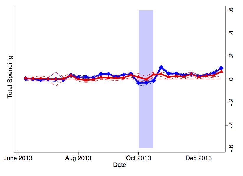
marital status, and the size of the household. Users also list whether they are a homeowner, their
profession, their level of education, their income level, and their location. Due to the nature of
the website, usage patterns suggest that it covers the entirety of financial transactions for groups
who make joint financial decisions. Thus, we equate a user of this financial website with a head-
of-household in the Current Population Survey (CPS) or a ‘consumption unit’ in the Consumer
Expenditure Survey (CES). For example, a ‘user’ represents the entirety of household spending
for married couples but only represents an individual’s spending for an unmarried individual living
with roommates.
    It is important to note that our identification strategy is local to government employees. It
is possible that consumption patterns differ for government employees and other groups. Our
sample is arguably representative of state and federal government employees in 2013. Being a
software start-up, in early years the demographics of the website were very different than those
of the nation as a whole. Key user characteristics like gender and age were starkly different than
the national distribution in 2007 (being younger and more male). While the demographics of the
user-base were initially very different, they have become much closer to a representative national
distribution by 2013 as the user-base grew dramatically. Moreover, conditional on observable
household demographic and locational characteristics, financial behavior among the users seems to
track closely to national averages. Moreover, the existing user-base differs from the population of
federal and state employees by less than it does from the total US population (eg. both have fewer
unbanked households or extremely high-income households). Summary statistics of the sample
population can be found in Table 3. Baker (2014) discusses using household weights derived from
CPS weightings and self-reported demographic and locational information in order to obtain more
externally valid estimates. Our results are robust to using equivalent household weights.

3    The Sensitivity of Consumption to Changes in Income
Our empirical strategy exploits the temporary drop in pay during the shutdown, and uses a dif-
ference in difference approach comparing affected federal government workers to unaffected state
government workers. Graphical evidence indicates that the two groups behave very similarly when
the shutdown was not in effect. The analysis sample used includes about 150,000 state and federal

                                                 9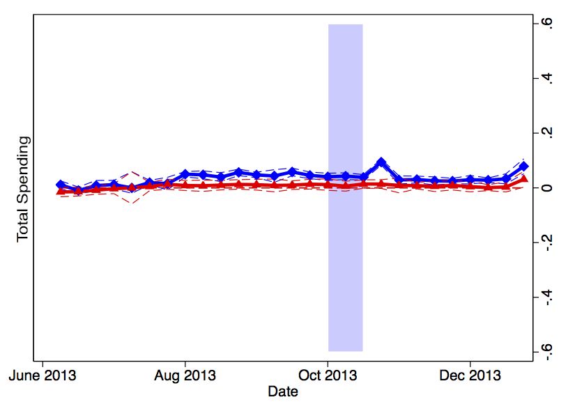
government employees in 2013. In our main specification, we estimate the following equations:

                                         T
                                               γj 1{j = t}t × 1{Gov}i + βXit + εit
                                         X
                    yit = αt + αi +                                                                (1)
                                         j=1

                                        T
                                               τj 1{j = t}t × 1{Gov}i + ζXit + ξit
                                        X
                     cit = ηt + ηi +                                                               (2)
                                         j=1

   where yit is income or log income, cit is spending or log spending and Xit are demographic
and other controls for individual i in time period t. Our coefficients of interest are the interactions
between 1{Gov}i , and an indicator of whether not an individual works for a federal government
agency that was affected by the shutdown and 1{j = t}t , a time period dummy. Let the subscript
s denote time periods when the government shutdown was in effect. We also include weekly time
period fixed effects αt to capture factors such as seasonality and time varying economic conditions,
as well as agency week fixed effects αi to capture unobserved time invariant differences between
workers and agencies.
   The terms εit and ξit represent mean zero error terms which are uncorrelated with the interac-
tion terms of interest conditional on observables. The identifying assumption is a parallel trends
assumption, that in the absence of the shutdown federal and state government workers income
and consumption patterns would have trended similarly. Graphical evidence from 2013 when the
shutdown was not in effect, as well as placebo tests in 2012 strongly support the validity of this
assumption as it is observed that federal and state government workers trend similarly.
                                   τs
   The ratio of the coefficients   γs
                                        provides us with an estimate of the sensitivity of consumption
to changes in income, where s denotes a period in which the shutdown is in effect. Estimated in
levels, the ratio can be interpreted as a marginal propensity to consume (MPC). We will estimate
analogous specifications of 1 and 2, replacing the dependent variable with logarithms of income
and spending to estimate the elasticity of consumption with respect to income. In a world in which
the permanent income hypothesis is valid, and agents are able to borrow and save freely, the MPC
resulting from a transitory negative income shock should be close to zero. If individuals are credit
constrained, the MPC can be as large as one.
   A large literature has found that there is excess sensitivity of consumption to changes in income,
which violates the canonical permanent income hypothesis. See Jappelli and Pistaferri (2010) for

                                                      10
a review of the literature. Many periods involving income changes, such as unemployment or
retirement, are associated with changes in time allocation. Changes in time allocation can also
affect consumption through multiple channels. The nature of the 2013 US government shutdown
allows us to go beyond testing for excess sensitivity, and use between-agency variation to separate
the effects of credit constraints and home production or leisure.
We add an interaction term for furloughed workers, 1{j = t}t × 1{Gov}i × P{F urlough}i ,
to equations 1 and 2. P{F urlough}i is the probability that a given worked was furloughed, which
is measured as the fraction of workers that were furloughed at the agency level. Table 2 shows the
fraction of workers furloughed at each agency. At some agencies like the Department of Education
and the Environmental Protection Agency, almost all workers were furloughed. At other agencies
such as the Department of Veteran Affairs and and Department of Agriculture almost no workers
were furloughed. The coefficient on the interaction terms gives the additional drop in consumption
for furloughed workers, who were subject to both a transitory loss of income as well as increased
leisure time and home production. Individual fixed effects are included to capture time invariant
factors specific to a particular worker.
One primary benefit of our data and identification strategy is that it is possible to separately
examine various types of household spending rather than only considering spending as a whole.
This allows for a greater understanding of household smoothing behavior and also lets us highlight
differences between households that were affected by the federal furloughs and loss of pay from
those solely affected by the loss of pay. We can also use the richness of the data and fine categorical
data to look for direct evidence of home production or leisure spending. We can re-estimate our
main specification separately for each category, including the triple difference furlough interaction.
If furloughed workers are engaging in home production, this would be evident through decreased
spending on items such as restaurants, child-related expenses or home and garden related expenses.
Evidence of increased leisure time could be present in categories such as entertainment, office
supplies and spending in venues related to leisure activities such as coffee shops or bars.
3.1 Was the Shutdown Anticipated?
One important consideration is the extent to which the government shutdown was anticipated by
households. Theory predicts that unanticipated and anticipated changes in income will have very
11different impacts on consumption. The permanent income hypothesis predicts that anticipated
income shocks should not have an effect on consumption, as individuals will save or dis-save
smoothly. The institutional framework of the 2013 government shutdown does not provide a clear
answer to the question of whether or not the shutdown was anticipated. While it was known that
the federal government would shut down if a continuing resolution was not passed, it is possible
that many workers predicted that a last minute deal would be reached as occurred several times in
debt ceiling negotiations.
We claim that the shutdown was largely unanticipated; despite high levels of polarization and
political uncertainty, there was no clear indication that the shutdown would actually occur. Sev-
eral similar standoffs led to last minute continuing resolutions that kept the government running.
In addition, other research often shows a lack of attention or understanding of economic news.
Eggers and Fouirnaies (2014) find that households strongly respond to the media announcing that
the economy is in a recession, leading to the conclusion that these households pay little attention
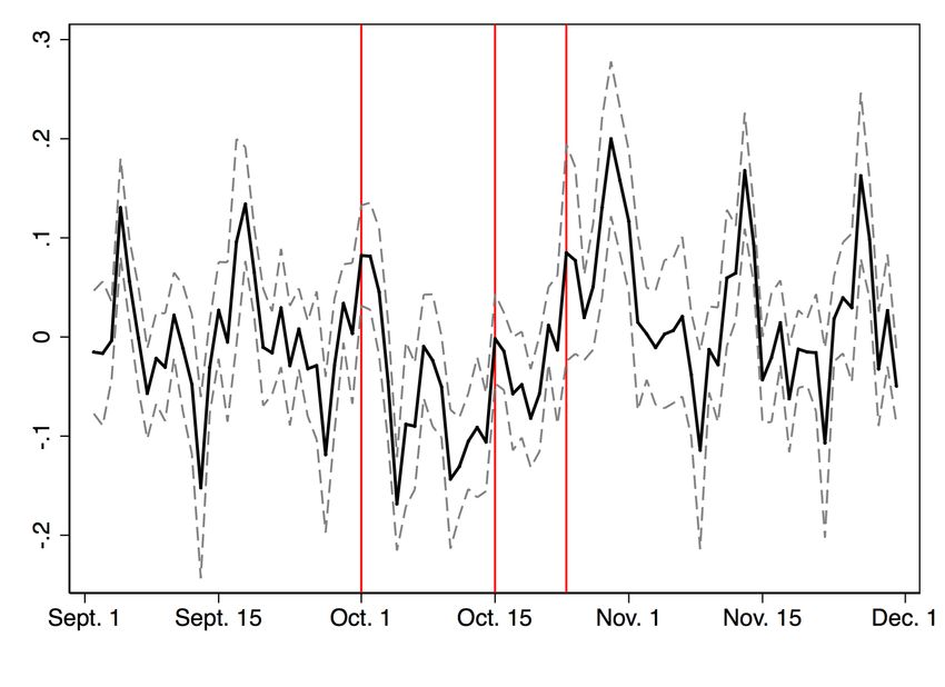
to economic fundamentals and only respond to the additional media attention. Figure 1 provides
suggestive evidence that the shutdown was not anticipated. The left panel displays the daily num-
ber of newspaper articles written that mention the phrase “government shutdown” as a fraction of
all newspaper articles from June 1st, 2013 to February 28th, 2014. Articles are queried using the
Access World News Newsbank database which is composed of almost 2000 newspapers in 2014.10
This graph indicates the dramatic surge in media attention paid to the government shutdown that
did not significantly precede the shutdown itself.
The right panel of Figure 1 focuses on the 3 weeks immediately preceding the government
shutdown. In blue is again the fraction of newspaper articles written that mention the shutdown. In
red is the probability of the shutdown occurring as calculated by the betting market website Inkling
Markets. The two series are highly correlated, with both series only seeing significant increases in
the 7 days leading up to the shutdown. This suggests that there was not a great deal of anticipation
by either the media or prediction market participants, who have been shown to be fairly accurate
predictors of political outcomes.11 Thus, it is unlikely that affected federal employees were able to
significantly alter their consumption and savings behavior in the short period before the shutdown
10
News query was run on June 15, 2014.
11
See Berg, Reitz, and Nelson (2008) and Wolfers and Zitzewitz (2006) for discussions of prediction market accu-
racy and interpretations.
12began and their income was disrupted.
We empirically test for any change in observable savings behavior using the following specifi-
cation:
T
ρj 1{j = t}t × 1{Gov}i + κXit + eit
X
sit = δt + δi + (3)
j=1
where sit is the amount individual i saved in period t. A test for whether or not the shutdown
was anticipated is ρi = 0 for all i = p where p denotes the three months before the shutdown. The
intuition behind this test is that if federal government workers could have anticipated the shutdown,
they would have saved to smooth consumption. We find no significant change in behavior leading
up to the shutdown. We find that, if anything, federal government workers save less than state gov-
ernment workers in the months preceding the shutdown although the difference is not significantly
different from zero. This provides additional evidence that the shutdown was not anticipated.
4 Results
We begin the analysis by documenting both a large income and corresponding spending response to
the shutdown. We then discuss various channels through which the shutdown impacted spending.
The observed pattern of the spending response is consistent with liquidity constraints, but not with
changes in expectations regarding permanent income. Changes in the time allocation of workers
also explain almost half of the decline in spending during the shutdown. Evidence from spending
categories indicates that both home production and increases in leisure could explain how changes
in time allocation impacted spending.
4.1 Income and Spending
Figure 2 displays variants of equations 1 and 2. The top row shows the coefficients for fixed effects
for each week for federal and state government workers, which are respectively the blue squares
and red triangles. Dashed lines show 95% confidence intervals for each point estimate. In the
left panel the dependent variable is income, while in the right hand panel the dependent variable
is spending during the final six months of 2013. The first three weeks of October, during which
13the shutdown affected incomes, is shaded. The left hand panel shows that the shutdown did affect
incomes significantly. In the second and third weeks of October 2013, there was an approximate
20-25% drop in incomes for federal government workers. The first week saw no impact due to the
fact that paychecks in the first week of October were for a full September pay period which still
was paid in full. The drop is followed by a rebound in the weeks following the shutdown. There
is a large spike in incomes in the final week of October, but we see smaller increases in November
and December which is consistent with a minority of workers not being repaid until later in the
year. There is no noticeable change in income for the control group, state and unaffected federal
government workers, which is expected as this group was not affected by the shutdown.
The right panel shows that the shutdown impacted spending. For federal government workers,
there is a small drop in the second period week of the shutdown, and a larger drop in the third week
of the shutdown. This pattern is consistent with credit constraints and federal government workers
exhausting their savings. The largest drop is seen in the third week of the shutdown, after the end
of the shutdown was announced. This pattern is not consistent with alternative explanations such
as the drop in spending being driven by revised beliefs about permanent income. Following the
shutdown, there is a rebound in spending. This rebound is driven primarily by durable purchases
and will be discussed further in section 4.2. Again we see no noticeable change in spending for the
control group, state government workers, which provides supporting evidence that the observed
patterns are not driven by seasonality.
The second row of Figure 2 shows the difference in difference specification in equations 1
and 2. Each point estimate shows the difference in the outcome for federal and state government
workers in the last six months of 2013. Dashed lines show 95% confidence intervals for each point
estimate. Both the income and spending differences for federal and state government workers are
statistically significant at the 0.05 level. The final row of Figure 2 repeats the analysis in the first
row for 2012, where the federal government did not shut down. In this placebo specification, there
is not a significant difference between federal and state government workers, providing supporting
evidence for our identifying assumptions and that the observed patterns are driven by the shutdown.
Note that we do observe some systematic statistically insignificant differences in spending patterns
between the federal government and state government workers. This is largely governed by the
fact that state and federal workers have somewhat different paycheck frequency such that there are
14some small within-month differences in spending between the two. However, as seen in the final
row of Figure 2, these differences are minor in general and especially so relative to the differences
seen during the shutdown.
Table 4 makes the graphical evidence presented in Figure 2 explicit. The first row shows
an interaction between the shutdown being in effect and an individual working for the federal
government. Column (1) indicates that the shutdown was associated with a 23.4 percent weekly
drop in income for federal government workers relative to state government workers. The drop
is significant at the 0.01 level. Column (2) shows the partial rebound in the week immediately
following the shutdown. The rebound is not full, since some federal government workers did not
receive backpay until November or December. Column (3) indicates that during the shutdown there
was an approximate 10.7 percent decrease in spending for federal government workers relative to
state government workers. The effect is significant at the 0.01 level. Column (5) shows that there
is a rebound in spending following the shutdown, however the rebound in spending is not as large
as the prior drop.
Column (4) adds a a triple interaction between the shutdown being in effect, an individual
working for the federal government and the probability that the individual was furloughed, 1[t =
Shutdown] ∗ 1[F edGov] ∗ P[F urlough]it where the subscript i denotes the individual and the
subscript t denotes the time period. The results indicate that the drop for furloughed workers is
roughly twice as large as that for workers who were not furloughed. This could be consistent
with either time allocation or home production affecting consumption, and this will be discussed
further in section 4.2.3. The results indicate a spending elasticity of consumption to income of
0.302 and a marginal propensity to consume of approximately 0.31. Column (1) shows that there
is no significant difference in the income decline for furloughed workers, suggesting that the results
are indeed driven by workers being sent home without pay during the shutdown. These results are
also depicted graphically, by fraction of workers furloughed at various agencies, in Figure 3.
Columns (6)-(8) collapse the results to the daily level by agency, providing an additional spec-
ification and robustness check. The results are quite similar to the main results and significant
at conventional significance levels. The results confirm that there is a large drop in spending for
federal government workers during the shutdown, relative to state government workers. Moreover
this drop in spending is much greater for workers who were furloughed during the shutdown. The
15results also confirm the rebound in spending following the shutdown.
4.2 Drivers of Spending Response
4.2.1 Differential Categorical Spending Declines
Table 5 breaks down the spending decline between various categories during the shutdown, along
with the differential decline for furloughed workers. The category is written above each column
and panel. The first row shows food related expenditures. For federal employees overall, there
is a significant decline in restaurant spending and no decline in fast food and grocery spending,
which may be more inelastic. There is a larger decline in fast food and grocery related spending
for furloughed workers. This could be due to home production, for example furloughed workers
could cook at home rather than eating fast food and spend more time preparing less costly meals.
The second row shows transportation related spending. For non-furloughed workers, there is
no decline in spending on public or auto transportation, or gasoline. Furloughed workers, who
stayed home during the shutdown see declines of between 1 and 8 percent in all transportation
related spending. The drops are significant at the 0.05 level or higher. This is evidence that the
shutdown did indeed impact the time use of workers. Exempted workers were required to work
during the shutdown, so we would expect to see no decline in transportation spending. Furloughed
workers were not allowed to attend work during the shutdown thereby cutting transportation and
commuting costs.
The third row of Table 5 shows spending results for shopping, clothing and check spending.
There is an approximate 6 percent drop in spending on clothing, and a 12 percent drop in check
spending for all government workers. The drops are significant at the 0.05 level or higher. Addi-
tionally there is a larger and marginally significant 7 percent drop in check spending for furloughed
workers, which could be consistent with reducing spending on services due to either home produc-
tion or changes in time allocation. There is no drop in shopping for exempted workers, however
furloughed workers see an approximate 7 percent drop in shopping.
The fourth row of Table 5 shows spending results for entertainment and home categories. There
is a 4 percent drop in cafe spending and a 1 percent drop in amusement spending for all federal
government workers. The drops are significant at the 0.05 level. There are increases in spending
16on cafes and amusement for furloughed workers, and the latter effect is significant at the 0.01 level.
This is consistent with changes in time allocation, as furloughed workers could spend money on
leisure activities rather than work and consumption. There is also evidence of home production,
as there is a marginally significant 1 percent decline in spending on home services. Furloughed
workers may have engaged in tasks such as raking leaves or childcare themselves as opposed to
hiring outside assistance.
The fifth and sixth rows of Table 5 provide placebo tests. At the 5 percent level, there is no
significant spending response in inelastic categories such as health insurance, auto and medical
payments, or education. We also see no significant spending response for exempted or furloughed
workers in interest income which should not be affected by the shutdown. The results in rows 5
and 6 provide further evidence that the observed effects are driven by a response to changes in
income and time allocation during the shutdown, and not other factors.
Figures 4 and 5 show graphical evidence of categorical spending declines. Figure 4 indicates
that, as in the main results, the timing of the observed drops and rebounds in spending is consistent
with the timing of the shutdown. The figure also provides support for the common trends assump-
tion. Figure 5 shows point estimates and 95% confidence intervals for shutdown and furlough
effects. The shutdown spending decline is largest in categories such as check spending, restaurants
and cash. Large declines in spending for furloughed workers are observed in categories such as
gas, fast food and check spending, and increases are observed in categories such as amusement and
personal care. This evidence is consistent with changes in time allocation and increases in leisure
impacting consumption.
Changes in time allocation can impact consumption through two non-mutually exclusive chan-
nels. First, if consumption and leisure are substitutes and non-separable, an increase in time avail-
able for leisure will reduce consumption. Second, individuals may engage in home production,
for example cleaning themselves rather than hiring outside help. Section 4.2.3 discusses the im-
plications of consumption responses due to home production or increased leisure. The categorical
spending declines provide evidence of both channels, however our design does not allow us to
quantify the impact of each channel on the time-allocation related decline in consumption.
174.2.2 Permanent Income
One important driver of the household consumption decision is the arrival of new information about
the future path of household income. Theory, and the well-established standard Euler equation
for consumption, tell us that households will react to unanticipated news about changes in their
permanent income path with a swift revision to their consumption with an elasticity near one.
Moreover, empirical work has consistently found strong impacts of unexpected permanent income
shifts.12
The government shutdown in 2013 may have changed households beliefs about the likelihood
that they would maintain steady increases in pay and about the security of their positions in both the
short- and long-run. The political crisis that precipitated the shutdown could have driven federal
employees to believe they may be more likely to be subject to furloughs, pay freezes, or more
intense political debates about public-sector compensation.
The standard Euler equation, along with the bulk of empirical research, would predict that a
downward shift in beliefs about permanent income would be accompanied by an immediate and
permanent decline in consumption equal to the size of the permanent income shock. That is,
affected households would decrease spending when their beliefs shifted and would not increase
spending to previous levels even after their temporary income disruption was relieved.
Examining figure 2 indicates that the timing of the consumption drop is inconsistent with re-
vised beliefs about permanent income. If federal government workers beliefs changed due to the
shutdown, we would expect to see an immediate drop in spending that was not followed by a re-
bound once the shutdown ended. This pattern is not what is observed. Instead, spending declines
over the month, consistent with home production or liquidity constraints and federal workers de-
pleting savings. In fact, the largest drop is during the third week of October, during which the end
of the shutdown was announced but workers had not received backpay. It is difficult to reconcile
this spending pattern with a model of the shutdown impacting beliefs about future income, while
12
Theory dating back to Friedman (1957) has posited diverging responses to transitory and permanent income
shocks. Flavin (1981), Campbell (1987), Carroll (2009) and Kaplan and Violante (2010) provide further theoreti-
cal justification for strong consumption responses to permanent income shocks in a wide range of settings. Work
including Gruber (1997), Wolpin (1982), Pistaferri (2001), Stephens (2001), Coulibaly and Li (2006) and Jappelli
and Pistaferri (2007) demonstrate these strong responses empirically. Stephens (2003) also examines the response to
known regular payments using the timing of Social Security benefits. This work, alongside many other papers, pro-
vides much evidence for large household consumption responses to permanent income shocks, although sometimes
finding responsiveness somewhat less than one, as theory would predict.
18the spending patterns are consistent with binding liquidity constraints.
We test this hypothesis formally by looking at income 3 months prior to the shutdown and 3
months afterward, when all foregone pay had been repaid to the households, and comparing federal
to state employees who were unaffected by the shutdown.13 We find no significant difference in
spending, at very high precision, allowing us to reject any long-lasting decline in household spend-
ing. Moreover, we find significant declines in spending during the shutdown, followed by a rapid
recovery in spending upon the ending of the shutdown, suggesting that the decline in household
spending was only temporary and likely not caused by shifts in permanent income expectations.
4.2.3 Consumption Types and Home Production
Changes in time allocation due to the shutdown could also affect consumption though multiple
channels. Theory predicts that if utility is non-separable in consumption and leisure, individuals
smooth the marginal utility of consumption, Et−1 [u(ci,t−1 , li,t−1 )] = u(ci,t , li,t ), and an adjustment
in leisure can lead to a consumption change. Home production can also cause a decline in observ-
able spending if more time is available. Both of these explanations have been noted, respectively
by Haider and Stephens (2007) and Aguiar and Hurst (2007) and Aguiar, Hurst, and Karabarbou-
nis (2013), as potential explanations for the sharp drop in consumption seen at retirement, counter
to the consumption smoothing predicted by the permanent income hypothesis. As well as being
of theoretical interest, the underlying reasons behind a time allocation response have important
welfare consequences in terms of designing social insurance programs. If the consumption drop
following unemployment is due to increased leisure rather than liquidity constraints, this has im-
plications in the design of optimal unemployment programs in the tradition of Baily (1978) and
Chetty (2006).
Other work by Guler and Taskin (2013) suggests similar effects hold for unemployment spells.
Burda and Hamermesh (2010), demonstrate cyclical variation in unemployment leads to variation
in home production but little impact on long-term unemployment. The framework of the 2013
government shutdown allows us to separate the effects of leisure and home production from other
13
One concern is that we find no significant differences here when looking at differential spending patterns between
affected federal workers and state government employees because of a strong correlation in the changes in income
expectations among these two groups. We also construct a control group composed of a random sample of private
sector workers at publicly traded firms. Using this as an alternate control, we find no evidence supporting a persistent
decline in income among the affected federal government employees.
19channels, since some workers were sent home while others were required to work without pay.
During the 2013 US government shutdown, some agencies furloughed nearly all of their work-
ers. Other agencies deemed services essential, and required the majority of employees to continue
working without pay. This latter group would have been unaffected by increased home production
or leisure, and hence any decline in consumption is more likely due to a credit constraint effect.
To identify the effects of credit constraints and home production or leisure, we estimate equations
1 and 2, adding an interaction term for the fraction of workers in an agency that were furloughed,
1{j = t}t × 1{Gov}i × P{F urlough}i . The coefficient on the interaction term provides an es-
timate of the difference in consumption that is driven from home production or leisure rather than
a temporary drop in income and credit constraints. A large negative coefficient is consistent with
changes in time allocation leading to a drop in consumption, which could be due either to leisure
or increased home production.
Column 4 of Table 4 is consistent with this pattern. The results indicate that while non-
furloughed federal workers saw a 7% decline in spending during the shutdown, those households
that had a furloughed worker saw spending decline by approximately twice as much. Column (2)
of Table 4 demonstrates that this larger decline in spending was in spite of any difference in how
household income was affected between these two groups. Observing particular types of spending
allows us to pin down the types of spending that led to this divergence.
To further examine whether the observed drop is due to home production or increased leisure
time, we can examine categorized spending data. Tables 5 and 6 show equation 2 broken down by
individual categories. There are large drops in categories such as eating out, shopping and office
supplies which are consistent with a number of interpretations. However, we see larger drops for
furloughed workers relative to exempted workers in categories such as dining out, groceries, baby
supplies, office supplies, entertainment and kid’s activities, which is consistent both with increased
leisure activity and home production in areas such as food preparation and child services.
Tables 5 and 6 also provide valuable placebo tests, which serve as a check regarding both our
empirical strategy and the validity of our category data. We do not see drops in consumption in cat-
egories that are unlikely to be cut due to a transitory income shock. We see no differential change
in health spending, which is likely to be inelastic and driven by adverse health shocks. We also see
no effect on auto payments, which could adversely affect credit scores and have large implications
20if missed. No effect is observed on interest income, which should be entirely unaffected by the
shutdown.
Table 5 displays results showing impacts on federal employees affected by the disruption in
pay during the shutdown as well as those affected by both the disruption in pay and the furlough.
At the top of column (1), for example, we see a decline in spending at restaurants across all
affected employees of approximately 8% as well as an additional negative and insignificant decline
in restaurant spending among furloughed employees of approximately 4%. In a number of the
categories in Table 5, we see differential household spending responses across affected employees
in general and furloughed employees in particular.
Consistent with an expected decline in commuting among the furloughed workers, we see sig-
nificantly less spending on automobiles, public transport, and gasoline compared to other affected
federal employees. We also see a larger decline in fast food and groceries expenditures. This may
be consistent with previous work suggesting that out-of-work individuals generally cut back on
consumption of food outside the home and also are able to shop for groceries more judiciously,
thus cutting expenditures while maintaining similar ‘consumption.’
In the third row, we find that furloughed households also did not experience the same decline
in spending on some categories of entertainment (eg. ‘Amusement’ as well as in the ‘Movies’ cat-
egory which is not enumerated in this table). This is evidence that households with additional time
away from work substituted into additional forms of entertainment outside the home. In contrast,
furloughed households saw declines in spending on home services like maids and babysitters. This
corresponds well with the increased ability of furloughed households to perform such household
labor themselves during the shutdown period. The fourth and fifth rows contain spending from
categories that may be more fixed in the short term. Households, either furloughed or exempted,
who were affected by the shutdown had little reaction to the shutdown in terms of their spending
on healthcare, car payments, or education payments.
4.2.4 Credit Constraints
The role of credit constraints in impacting household consumption behavior is often highlighted
when examining unexpected declines in income. In the classic permanent income hypothesis
framework, unexpected temporary declines in income only manifest themselves as declines in
21consumption if households are credit or liquidity constrained.14
Given most affected federal employees knew that they would be repaid all foregone income
following the conclusion of the government shutdown, they would experience no expected change
in lifetime income. Because they would only be subject to a temporary decline in income, this
framework would predict a decline in consumption only among those households who were un-
able to borrow or draw on liquid savings to smooth their consumption during the shutdown until
their regular income resumed. Unable to borrow or draw on savings to finance current consump-
tion, constrained households would be predicted to cut and defer spending during the government
shutdown. Thus, any decline in spending would be only seen among households without sufficient
savings or borrowing capability.
Suggestive evidence of credit constraints playing a role in the consumption drop is presented
in Table 7. The table provides additional categorical specifications, broken down at the daily level
for each agency. We aggregate across individuals in each agency in this specification due to the
fact that there are large numbers of observations with zero spending at a day-category level. The
first three columns (where columns 1 and 2 are in logs and column 3 in levels) show aggregate
spending before and after the shutdown and confirm the patterns seen earlier– there is a drop
in spending for federal government workers during the shutdown, and a rebound following the
shutdown when backpay was received. Columns 4-8, in logs, confirm that a similar pattern is seen
across all categories in the table: durables, non-durables, services, dining, and mortgage spending.
The rebound following the shutdown, while significant, is much smaller for the dining category.
The fact that there is a decline and corresponding rebound in mortgage spending suggests re-timing
in the paying of bills.
The second row of Table 7 presents an indicator for the time period in between the announce-
ment of the shutdown and the first post-shutdown paychecks arriving. The third row of the table
shows an indicator for the final week of October, when the post shutdown paychecks arrived with
14
See, for instance, Bishop and Park (2011) which demonstrates that marginal propensities to consume drop steeply
following a relaxation in binding borrowing constraints. Kaplan and Violante (2014) and Eggertsson and Krugman
(2012) both spell out mechanisms by which credit or liquidity constrained households become more responsive to
income changes with potential macroeconomic consequences. Zeldes (1989), Johnson, Parker, and Souleles (2006),
Souleles (2000b), Souleles (2000a) and Blundell, Pistaferri, and Preston (2006) also estimate a higher level of con-
sumption elasticity among households with less credit and net worth. In addition, recent work has suggested a poten-
tially large role of credit constraints in the consumption decline seen during the Great Recession (eg. Baker (2014),
Mian, Sufi, and Rao (2013) and Dynan (2012).
22You can also read