INFLUENCE OF RANGING UNCERTAINTY OF TERRESTRIAL LASER SCANNING ON CHANGE DETECTION IN TOPOGRAPHIC 3D POINT CLOUDS
←
→
Page content transcription
If your browser does not render page correctly, please read the page content below
ISPRS Annals of the Photogrammetry, Remote Sensing and Spatial Information Sciences, Volume V-2-2020, 2020
                                                 XXIV ISPRS Congress (2020 edition)

INFLUENCE OF RANGING UNCERTAINTY OF TERRESTRIAL LASER SCANNING ON
        CHANGE DETECTION IN TOPOGRAPHIC 3D POINT CLOUDS

                                            L. Winiwarter1, ∗, K. Anders1,2 , D. Wujanz3 , B. Höfle1,2
         1
             3D Geospatial Data Processing Research Group (3DGeo), Institute of Geography, Heidelberg University, Germany
                      2
                        Interdisciplinary Center for Scientific Computing (IWR), Heidelberg University, Germany
                                        3
                                          Technet GmbH, Am Lehnshof 8, 13467 Berlin, Germany

                                                            Commission II, WG II/10

KEY WORDS: Uncertainty, Error propagation, M3C2, Significance, Statistical Test

ABSTRACT:

Terrestrial laser scanners are commonly used for remotely sensing natural surfaces into 3D point clouds. Time series of such 3D
point clouds can be analysed to gain information of surface changes that are induced by Earth surface shaping processes. The
atomic unit in time series analysis is a bitemporal change detection and quantification. This should involve an estimation of the
minimum quantifiable change, the Level of Detection, to separate signal from noise, e.g. stemming from the measurement. To
enable such an estimation through error propagation, a model of the sensing instrument’s measurement uncertainty is required. In
this work, we present an investigation on the ranging component of terrestrial laser scanning on this uncertainty and its influence
on 3D distances between point clouds of two epochs. Specifically, we analyse the effects of incidence angle, intensity and range
for different object materials, and make additional considerations with respect to waveform information returned by the sensor. We
estimate a model for the rangefinder uncertainty of a terrestrial laser scanner and apply it on experimental data. The results show
that using a sensor-specific model of ranging uncertainty allows an appropriate estimation of the Level of Detection. At a range of
60 m and a rotational displacement of 10◦ , this Level of Detection ranges between 0.1 mm to 1 mm for a white and a grey surface
and up to 5 mm for a black surface. The completeness of the detection of significant change ranges from 60.2 % (black) to 89.8 %
(grey) for the proposed method and from 65.5 % to 88.9 % for the baseline, when compared to tachymeter measurements. The
similarity between the results is expected and suggests the validity of error propagation for the derivation of the Level of Detection.

                       1. INTRODUCTION                                      to this uncertainty model for a photogrammetric point cloud by
                                                                            using ”precision maps” which map a spatially variable coregis-
The availability of high-resolution topographic 3D point cloud              tration uncertainty to the dataset. Still, the per-point uncertainty
time series has enabled the detection and quantification of                 is only estimated from the data and its fit to a planar model.
changes in surface geometry (Eitel et al., 2016; Fey and Wich-
mann, 2017; Zahs et al., 2019). These 3D point clouds are un-               On the sensor side, multiple studies have investigated the influ-
ordered, irregular sets of points in 3D space acquired, e.g., by            ence of parameters like incidence angle (Soudarissanane et al.,
terrestrial laser scanning (TLS). TLS sensors are used to re-               2007; Kersten et al., 2009; Zámečnı́ková et al., 2014), colour
peatedly sample the Earth’s surface, but the exact locations of             (Clark and Robson, 2004; Mechelke et al., 2007) and intensity
the sampled points differ from scan to scan and therefore from              (Pfeifer et al., 2007; Wujanz et al., 2017, 2018) on the ranging
epoch to epoch. To obtain a reliable measure of surface change,             precision of laser scanners. Furthermore, Fey and Wichmann
points are aggregated to local surface models. Often, a loc-                (2017) have quantified how range and incidence angle influence
ally planar surface is assumed. The most developed method to                the positional uncertainty of 3D laser scanning points, and have
quantify distances between two point clouds for geographic ap-              applied their findings to geomorphic change detection in alpine
plications is the multiscale model-to-model cloud comparison                terrain.
(M3C2, Lague et al., 2013), which directly compares two point
clouds by such a locally planar model.                                      These studies suggest that a combination of the models derived
                                                                            from the sensing process and from data analysis could lead to
To separate real change from change values stemming from                    a better understanding of the distribution of measurement un-
measurement and other noise, statistical tests can be employed.             certainties throughout a dataset. Knowledge of these uncertain-
Lague et al. (2013) estimate the required second-order moments              ties can then be used to estimate the resulting uncertainty in a
by modelling the laser rangefinder uncertainty1 from the dis-               change analysis, allowing for a clear separation of measurement
tribution of points in the local point cloud neighbourhood. A               noise and change signal.
coregistration term accounts for the misalignment of the data-
sets of the two epochs. James et al. (2017) present an extension            We therefore perform an experiment to investigate the influence
∗
                                                                            of material, range and incidence angle on intensity, pulse shape
    Corresponding author
1                                                                           deviation and, most prominently, ranging uncertainty (i.e., ran-
    We take care to use the term ”uncertainty” as defined in the Guide to
    the expression of uncertainty in measurement: ”The uncertainty [...]    ging precision), with the goal of detecting change in a bi-
    reflects the lack of exact knowledge of the value of the measurand”     temporal dataset acquired with TLS. Subsequently, we create
    (JCGM, 2008), in contrast to ”error”, which is ”an idealized concept    a model that allows the estimation of the ranging uncertainty
    and [...] cannot be known exactly” (JCGM, 2008).                        for each point of the point cloud individually. We show how to

             This contribution has been peer-reviewed. The double-blind peer-review was conducted on the basis of the full paper.
                         https://doi.org/10.5194/isprs-annals-V-2-2020-789-2020 | © Authors 2020. CC BY 4.0 License.                        789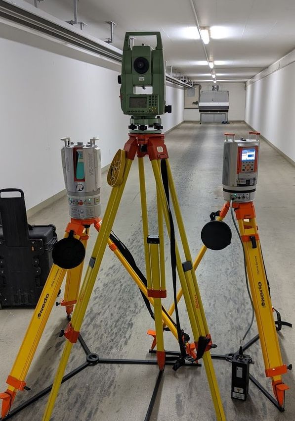
ISPRS Annals of the Photogrammetry, Remote Sensing and Spatial Information Sciences, Volume V-2-2020, 2020
                                               XXIV ISPRS Congress (2020 edition)

use this estimation in a change detection analysis and present
the applicability of our method by comparing our results to the
state-of-the-art method of M3C2.

                         2. METHODS

2.1    Experimental design

To evaluate the influence of different object and sensing proper-
ties, we conducted an experiment under controlled conditions.
This consisted of scanning a locally planar wooden board at
different ranges and different incidence angles. Additionally,
we covered the board with dull plastic foil (black and white)
and toned paper (grey), resulting in different reflectance values.
The reflectance at approximately 0◦ incidence angle was cal-
ibrated by using a target with known reflectance (SphereOptics
Zenith LITE with a reflectivity of 92.5 % at λ = 1550 nm) at
the same range. The resulting values are listed in Table 1.
          Material      Black foil    Grey paper     White foil
   Reflectance [%]      83.66         89.33          94.92
     Std. dev. [%]      2.09          1.44           1.42
                                                                        Figure 1. Measurement setup. Left: RIEGL VZ-2000i, center:
      Table 1. Reflectance values at 0◦ incidence angle for the
                                                                            Leica TCRA705power, right: RIEGL VZ-400. In the
                     different surface materials.
                                                                         background, the experiment board can be seen at a range of
The wooden board was mounted in an upright (vertical) posi-              30 m. The experiment was carried out in a basement which
tion, and subsequently rotated from normal to the laser beam                   allows a maximum target range of about 250 m.
(0◦ ) to angles of up to 60◦ , in increments of 10◦ . Via this ro-
tation, we cover a number of different incidence angles of the
laser beam. We define the incidence angle as the angle between
the inverted beam vector and the local surface normal vector
oriented towards the scanner. Furthermore, the rotation acts
as controlled displacement for the surface change quantifica-
tion. The scans of all seven rotations were repeated for ranges
of about 30, 60, 90, 160 and 220 m, resulting in a total of 35
scans.

As a reference for the displacement quantification, eight retro-
reflective targets were installed on the board and measured with
a tachymeter (Leica TCRA705power). During the TLS scans,
we covered the targets to avoid any interferences. Since dis-
placement only regards relative movement, the total station was
not tied in with the TLS coordinate system, but we assume the
scale of both systems to match. The experiment was carried out
under controlled atmospheric conditions in a basement with ar-
tificial lighting, and with two different TLS instruments (RIEGL
VZ-400 and RIEGL VZ-2000i). The measurement setup is
shown in Figure 1.

To ensure that the recorded noise stems from the sensor and not
from roughness in the surface itself, we used a sanded OSB-3             Figure 2. Wooden board with white, grey and black surface
wooden board, which has a tolerance in thickness of 0.3 mm             materials. The reflective tape markers along the edges are used
according to EN300 (DIN, 2006). This is an order of magnitude           for the tachymetry. The image shows the board at an offset of
lower than the expected ranging precision given by the TLS                 approximately 20◦ with respect to the ranging direction.
manufacturer, which is 3 mm at 100 m range for both employed           Refelections can be seen in the black surface, indicating that the
TLS systems (RIEGL LMS, 2019). Figure 2 shows the board                                   surface is not Lambertian.
in the measurement environment.

2.2    Modelling range uncertainty                                     to a circle with a radius of approx. 3 cm at 60 m range with the
                                                                       used scan parameters) is then used to define the local plane for
We evaluate the ranging uncertainty by calculating the offset          each point using a least-squares optimization, which allows us
of individual point measurements from the locally best fitting         to disregard potential low-magnitude but large-scale deforma-
plane. First, the 3D points on the board are manually segmen-          tions like a bend of the board.
ted from the full point cloud and separated into the three surface
materials. A local neighbourhood of 10 points (corresponding           We then project the quality of the plane fit (σ0 , i.e. standard

           This contribution has been peer-reviewed. The double-blind peer-review was conducted on the basis of the full paper.
                       https://doi.org/10.5194/isprs-annals-V-2-2020-789-2020 | © Authors 2020. CC BY 4.0 License.                   790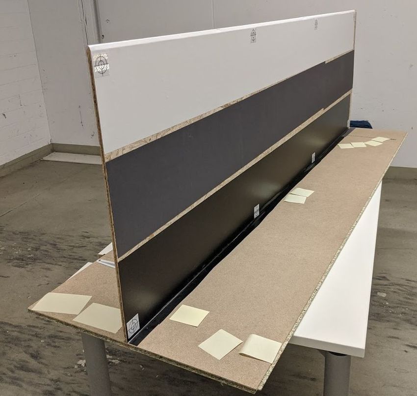
ISPRS Annals of the Photogrammetry, Remote Sensing and Spatial Information Sciences, Volume V-2-2020, 2020
                                             XXIV ISPRS Congress (2020 edition)

deviation of the points in the local neighbourhood in direction
of the plane normal vector) onto the beam vector of the neigh-
bourhood centroid to get an estimate of the ranging precision.
Since our ranging distance is large compared to the extent of the
board, we average the ranging precision per surface material.

In addition to the range and angular measurements of the TLS,
we record the signal intensity Int and the pulse shape deviation
Dev . In accordance with RIEGL LMS (2012), we define the
intensity to be a unitless [dB] measure of the amplitude of the
returned signal without any corrections corresponding to range
or incidence angle normalized to 16 bits. The pulse shape devi-
ation is a unitless measure of how similar the outgoing and the
incoming pulses are shaped, and can therefore be related to the
quality of the range measurement.

With the 35 estimates of ranging uncertainty made at five differ-        Figure 3. Change detection and quantification schema. The
ent ranges and seven different incidence angles respectively, we         distance d is calculated orthogonal to the board position at
use a least squares method to create a model of linear combin-                                     Epoch 1.
ation for the estimation of the ranging uncertainty. The inputs
to this model are the cosine of the incidence angle, the devi-       respectively. The term reg. is an additional constant coregistra-
ation and the recorded intensity. In accordance with Wujanz          tion uncertainty, which is neglected in this experiment because
et al. (2017), we rely on the range equation (Eq. 1) to model        of the static setup, since the scanner was not moved during the
the change in range implicitly via the change in intensity. To       acquisitions at a constant range.
test this assumption, we add the range as a separate input and
analyse the correlation between the parameters.                                                      r
                                                                                                       σ1   σ2
                                                                                 LoDetection95 = 1.96     +    + reg.                  (2)
                                                                                                       n1   n2
                         Pt Dr4
                   Pr =          ηsys ηatm σ                  (1)
                        4πR4 β 2
                                                                     Instead of applying Equation 2, we propose to propagate the
                                                                     ranging uncertainty from the TLS to the individual laser points.
                                                                     Since it extends the M3C2 algorithm by error propagation2 , we
where       Pr = received signal power                               refer to it as M3C2-EP.
            Pt = transmitted signal power
            Dr = diameter of receiver aperture                       We estimate a full covariance matrix for the local neighbour-
            R = range from sensor to target                          hood centroids of each epoch. Since we are looking for sig-
            β = beam divergence                                      nificant change in the specific direction normal to the planar
            ηsys = system efficiency                                 surface, we subject this matrix to a projection onto the normal
            ηatm = atmospheric transmission factor                   vector ~n and derive a Level of Detection using a test statistic,
            σ = target cross section                                 which is distributed according to Hotelling’s t-squared distri-
                                       (Jelalian, 1992)              bution (Rencher, 1998). This distribution can be related to an
                                                                     F-distribution, giving the expression in Equation 3. This corres-
2.3   Change detection and quantification                            ponds to a two-sided test of multivariate normally distributed
                                                                     means with p = 3 degrees of freedom.
We first quantify change between point clouds by using the
common M3C2 point cloud distance measure (Lague et al.,                                            s
                                                                                                       F0.95 (p, n1 + n2 + 1 − p)
2013). It aggregates points within a local neighbourhood                      LoDetection95 =                            n1 +n2 +1−p
                                                                                                                                       (3)
formed by a cylinder oriented along the local normal vector                                             ~nT Ĉ −1 ~n ·    (n1 +n2 )p
of the reference epoch point cloud. The points within these
local cylinders are then projected onto the cylinder axis for each
epoch separately, where the difference between their mean po-        Here, Ĉ is the pooled covariance matrix (Eq. 4), n1 and n2
sitions is used as a distance measure. The standard M3C2 then        are the number of points, and C1 and C2 are the covariance
uses the standard deviation of the points along the cylinder axis    matrices for the respective epochs.
as a precision measure.
                                                                                                  1
In our experiment, we use the board at a 0◦ incidence angle,                            Ĉ =           (C1 n1 + C2 n2 )                (4)
                                                                                               n1 + n2
with the board normal to the laser beam, as reference epoch, and
quantify change orthogonal to this epoch, as shown in Figure 3.
                                                                     To achieve full 3D per-point uncertainties in the form of co-
Subsequently, we detect significant change as a binary label us-     variance matrices for each laser point, we assume the scan-
ing a two-sided t-Test. This test can be reformulated to find the    ner to have an angular standard deviation defined mainly by
minimum quantifiable change, referred to as the Level of De-         the laser beam divergence. This neglects the influence of the
tection (LoDetection, Eq. 2). Here, σi refers to the standard de-    2   Because of the common use of the term ”error propagation” (cf.
viation of the points along the cylinder axis and ni to the num-         JCGM, 2008, Section E.3.2), we do not refer to it as ”uncertainty
ber of points within the cylinder, for epochs i = 1 and i = 2,           propagation”, even though this formulation would be more precise.

         This contribution has been peer-reviewed. The double-blind peer-review was conducted on the basis of the full paper.
                     https://doi.org/10.5194/isprs-annals-V-2-2020-789-2020 | © Authors 2020. CC BY 4.0 License.                       791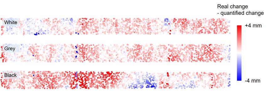
ISPRS Annals of the Photogrammetry, Remote Sensing and Spatial Information Sciences, Volume V-2-2020, 2020
                                              XXIV ISPRS Congress (2020 edition)

angular measurement resolution, in contrast to the work by                3.1   Dependencies between ranging uncertainty, range, in-
Lichti and Jamtsho (2006). For the specific scanner used,                       cidence angle, intensity and pulse shape deviation
the beam divergence accounts for most of the angular uncer-
tainty. According to the datasheet, the beam divergence of                In order to find a functional model describing the ranging un-
the RIEGL VZ-2000i is 0.27 mrad (0.3 mrad for the RIEGL                   certainty, we examine how different measures provided by the
VZ-400), and is defined at the 1/e2 points of the energy                  rangefinding system itself (intensity, range, and deviation) and
distribution. Assuming a constant reflectance of the board                by the data (incidence angle) correlate with each other and with
within a single laser footprint, we use a quarter of this beam            the ranging uncertainty.
divergence as standard deviation in scan and yaw angles:
σScan = σY aw = 0.27 mrad/4 = 0.0675 mrad.                                Figure 4 shows a scatter plot between ranging uncertainty and
                                                                          range for the VZ-2000i system at a constant incidence angle
Since the scanners were not moved when changing the incid-                of about 0◦ . The curve shows a clear trend for all three ma-
ence angle, we disregard any terms concerning the coregistra-             terials that the ranging uncertainty increases with larger ranges.
tion, leading to a simple functional model for the error propaga-         Similarly, the ranging uncertainty decreases for increasing in-
tion, as shown in Equation 5. Here, ϕ represents the yaw angle            tensities, as shown in Figure 5.
(horizontal), θ the scan angle (vertical), r the range and (x, y, z )
the cartesian coordinates for each point i.

    (x, y, z)Ti = ri · (cos ϕi sin θi , sin ϕi sin θi , cos θi )T   (5)

By comparing the quantified change with the reference change
measured by tachymeter, we can evaluate the detection metric
in form of a confusion matrix, as shown in Table 2. We assume
change to be significant (i.e. detectable) if the change calcu-
lated from the tachymeter measurements is greater than or equal
to the estimated LoDetection of the respective method, and to             Figure 4. VZ-2000i ranging uncertainty vs. range for a constant
be indistinguishable from noise otherwise. This significance                                  incidence angle of 0◦ .
is then compared to the one from the statistical test using the
quantified change by means of correctness and completeness
(Eq. 6). Here, ”TP” refers to a change calculated by tachymeter
measurement that is larger than the associated LoDetection and
is estimated as significant from the TLS point cloud. ”FP” is a
change that is estimated as significant from the TLS data, but
is not larger than the LoDetection when calculated from tachy-
metry. Similarly, ”TN” and ”FN” refer to changes estimated as
not significant and are smaller and larger or equal to the LoDe-
tection (when change is calculated from tachymetry), respect-
ively. The LoDetection is always derived from the TLS data.
                                       Reference
                            LoDetec. ≥ real LoDetec. < real
                                                                            Figure 5. VZ-2000i ranging uncertainty vs. intensities for a
         Significant        TP               FP
 Est.    Insignificant      FN               TN                                          constant incidence angle of 0◦ .

 Table 2. Comparison between significance from estimation and             The similar patterns in Figures 4 and 5 suggest that much of the
tachymeter control measurements in form of a confusion matrix.            influence of different ranges on the ranging uncertainty can be
 The reference significance is created by comparing the Level of          modelled adequately by the drop in intensity, as given by the
  Detection estimated from the point cloud with the real change           range equation (LiDAR Equation, Eq. 1). To verify this, we
                    measured by tachymeter.                               show the decrease of intensity with respect to range in Figure 6.

                                                                          Similar observations can be made for intensities and incidence
                                    TP
                      Correctness =                                       angles, where the intensity decreases with an increasing incid-
                                  TP + FP                                 ence angle (Fig. 7). However, the quality of the plane fit and
                                                                    (6)
                                    TP                                    also of the projected ranging uncertainty exhibit different beha-
                   Completeness =
                                  TP + FN                                 viours for different surface materials. For the black surface, the
                                                                          ranging uncertainties increase with increasing incidence angles
              3. RESULTS AND DISCUSSION                                   as would be expected and was also shown in previous studies
                                                                          (e.g. Soudarissanane et al., 2007), even if the effect is more
We first present dependencies between different factors of influ-         prominent with phase scanners than with time-of-flight scan-
ence by visual analysis of respective scatterplots in Section 3.1.        ners like the RIEGL sensors (Kersten et al., 2009). But for the
Subsequently, a ranging uncertainty model is estimated from               grey and white surfaces, the uncertainties decrease for incid-
the data (Section 3.2), which is then used and validated in er-           ence angles above about 20◦ (Fig. 8). This behaviour is similar
ror propagation for the detection of significant change in Sec-           for all ranges, and suggests that the type of material influences
tion 3.3.                                                                 the ranging precision going beyond just the strength of returned

          This contribution has been peer-reviewed. The double-blind peer-review was conducted on the basis of the full paper.
                      https://doi.org/10.5194/isprs-annals-V-2-2020-789-2020 | © Authors 2020. CC BY 4.0 License.                       792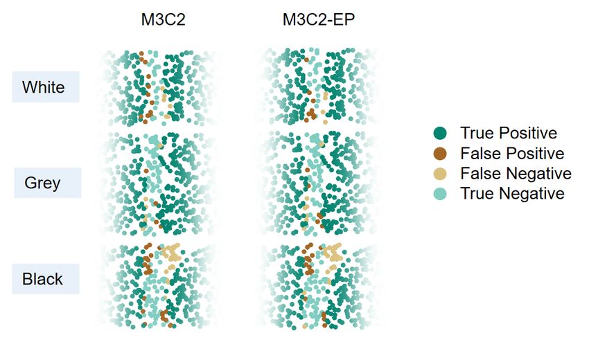
ISPRS Annals of the Photogrammetry, Remote Sensing and Spatial Information Sciences, Volume V-2-2020, 2020
                                              XXIV ISPRS Congress (2020 edition)

 Figure 6. VZ-2000i recorded intensity vs. range for a constant        Figure 9. VZ-400 ranging uncertainty vs. incidence angle for a
                    incidence angle of 0◦ .                                              constant range of 60 m.

signal, i.e. that the material is not behaving like a Lambertian
reflector. This suggestion is further supported by the fact that
especially the black foil has specular reflective properties as vis-
ible in Figure 2. For the black surface, only three data points are
available, since no points were recorded for incidence angles
above 20◦ at the range of 60 m.

                                                                         Figure 10. VZ-400 plane fit quality vs. incidence angle for a
                                                                                          constant range of 60 m.

Figure 7. VZ-2000i recorded intensity vs. incidence angle for a
                  constant range of 60 m.

                                                                       Figure 11. VZ-2000i deviation vs. incidence angle for a constant
                                                                                              range of 60 m.

                                                                       In addition to the polar measurements and the intensity, the
                                                                       scanners deliver information on how the received pulse shape
                                                                       deviates from the outgoing one. Plotting this deviation as a
Figure 8. VZ-2000i ranging uncertainty vs. incidence angle for a       function of the incidence angle shows a similar pattern to the
                   constant range of 60 m.                             ranging uncertainty (Fig. 11), suggesting that the deviation can
                                                                       be used, at least in part, to explain the behaviour of a decreasing
                                                                       ranging uncertainty for high (flat) incidence angles.
The data recorded with the RIEGL VZ-400 shows a similar pat-
tern (Fig. 9), with the maximum ranging uncertainty shifted to-        Similarly, a plot of the ranging uncertainty as a function of the
wards higher incidence angles. Still, the ranging uncertainty          pulse shape deviation shows higher ranging uncertainties with
decreases for higher incidence angles. However, this can be ex-        a larger pulse shape deviation for the grey and the white sur-
plained by the projection of the plane fit onto the beam vector        faces as expected, but an inverted effect for the black surface
reducing the uncertainty by the cosine of the incidence angle          (Fig. 12), that we again attribute to the non-Lambertian proper-
(where the angular uncertainty starts to contribute more to the        ties of the material.
total positional uncertainty). We also plot the quality of the
plane fit against the incidence angle (Fig. 10). This shows an al-     3.2   Ranging uncertainty model
most linear relationship, which fits the theoretical expectation.
For the RIEGL VZ-2000i, this relation is not that prominent,           The observations presented in Section 3.1 indicate that a single
but the decrease of the ranging uncertainty with increasing in-        model is not sufficient to adequately describe the ranging un-
cidence angles (Fig. 8) is partly explained.                           certainty for all three surface materials. Instead, each surface

         This contribution has been peer-reviewed. The double-blind peer-review was conducted on the basis of the full paper.
                     https://doi.org/10.5194/isprs-annals-V-2-2020-789-2020 | © Authors 2020. CC BY 4.0 License.                      793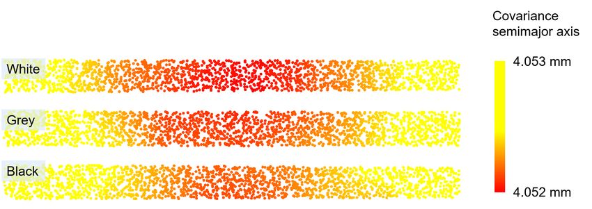
ISPRS Annals of the Photogrammetry, Remote Sensing and Spatial Information Sciences, Volume V-2-2020, 2020
                                             XXIV ISPRS Congress (2020 edition)

                                                                     only data for low incidence angles is available, limiting the
                                                                     model’s ability to separate the influence of incidence angle from
                                                                     a constant term, validating our assumptions.

                                                                     3.3   Error propagation and assessment of significant
                                                                           change

                                                                     We apply the model presented in Section 3.2 to the original
                                                                     point cloud, generating a stochastic point cloud in accordance
                                                                     with Wujanz et al. (2017). In order to investigate the ranging
                                                                     uncertainty as the major contribution in the uncertainty of the
                                                                     change quantification, we calculate changes of the rotated board
  Figure 12. VZ-2000i ranging uncertainty vs. deviation for a        with respect to the 0◦ position, and look for changes along the
                  constant range of 60 m.                            normal vector of this position (see Fig. 3).

                                                                     Because of the noise in the intensity and deviation signals, the
individually exhibits its own material properties which influ-       resulting per-point covariance varies in small neighbourhoods.
ence the ranging uncertainty. Therefore, we estimate a function      However, since the M3C2 algorithm includes an aggregation,
σr = f (. . .) separately for each surface material. This also       these variations are averaged out when testing for significant
covers the difference in colour, i.e. reflectance at λ = 1550 nm,    changes between the two epochs. Figure 13 shows the per-point
as described by Clark and Robson (2004).The TLS system fur-          covariance by means of the semimajor axis of the error ellipsoid
ther has specific characteristics, especially concerning the (un-    for one scan after this aggregation step. The different materi-
corrected) intensity signal. Therefore, individual models have       als show specific patters of their respective ranging uncertainty
to be created for different TLS models (Wujanz et al., 2017,         models. Since the incidence angle is assumed constant in this
2018).                                                               example and local variations in intensity and deviation are aver-
                                                                     aged out within the search cylinders, the only remaining influ-
We choose f = a + b · Int with unknown parameters a and b
                                                                     ence is the range - which is slightly (i.e., by a few mm) larger
and the recorded intensity Int as a starting point for our model.
                                                                     at the edges of the board. Therefore, Figure 13 shows the de-
In contrast to Wujanz et al. (2018), we do not model an addi-
                                                                     pendency of the uncertainty by range, only changing by a few
tional parameter in the exponent of Int, because this did not
                                                                     micrometers across the board.
lead to a converging solution with our data. Still, we expect this
function to adequately model the influence of different meas-
urement ranges, as these explain much of the variation in the
intensity (see Fig. 6). Additionally, we consider the cosine of
the incidence angle cos(ϕ) and the pulse shape deviation Dev
as additional linear influences with factors c and d. The full
model is stated in Equation 7.

           σr = a + b · Int + c · cos(ϕ) + d · Dev             (7)
                                                                      Figure 13. Semimajor axis of the error ellipsoid estimated for
                                                                       the scan at 60 m range and 0◦ incidence angle. The different
The parameters for the different surfaces are estimated for the       models for the different materials show different patterns, even
RIEGL VZ-2000i using a least-squares method on all available          though the absolute values are not affected much in this setup.
data. The results are listed in Table 3.
               â [m]          b̂ [m]      ĉ [m]          dˆ [m]    We show the differences between the reference change and the
 White      0.00175     -3.54 ·10−7     0.00253      1.27 ·10−5      quantified change for an increase of incidence angle from 0◦
  Grey      0.00333     -4.71 ·10−7     0.00207     -4.40 ·10−5      to 10◦ in Figure 14. The reference change was calculated by
 Black     -0.00223     -6.48 ·10−7     0.00875     -1.75 ·10−4      fitting 2.5D quadrics to the tachymeter measurements in the re-
                                                                     spective epochs, sampling points on these surfaces and then ap-
  Table 3. Estimated coefficients for the three different surface    plying M3C2. The same sampled points are then used as neigh-
 types. These values are subsequently used in the estimation of      bourhood query centers for the subsequent, point cloud-based
           per-point uncertainty in ranging direction.               analysis. By comparing the quantified change to the estimated
                                                                     LoDetection, significant change is identified. The quantified
An analysis of the correlation matrix of the estimated paramet-      change is calculated using the M3C2 algorithm with a search ra-
ers for the white surface shows a maximum absolute correlation       dius of 5 cm. The normal vectors are taken from the artificially
of 0.46 between parameters a (the constant term) and d (the de-      sampled point cloud at approximately 0◦ incidence angle.
viation dependent term). When including the range as an addi-
tional linear parameter, the respective coefficient highly correl-   Two different charts of significant change are shown in Fig-
ates (0.92) with parameter b, the amplitude dependent term.          ure 15 for a part of the board. The detection of significant
                                                                     change between the standard M3C2 and our method with error
The models for the other surfaces exhibit slightly higher cor-       propagation is practically equal. Additionally, the difference of
relations, especially the one for the black surface, where a and     the LoDetection is shown in Figure 16, where our method es-
c (the constant term and the incidence angle-dependent term)         timates a much more homogeneous LoDetection for all surfaces
correlate with a coefficient of 0.95, even without including the     than the baseline model. By comparing the estimated LoDetec-
range dependent term in the model. This is not surprising, as        tion to the change quantified by the tachymeter, we estimate a

         This contribution has been peer-reviewed. The double-blind peer-review was conducted on the basis of the full paper.
                     https://doi.org/10.5194/isprs-annals-V-2-2020-789-2020 | © Authors 2020. CC BY 4.0 License.                   794
ISPRS Annals of the Photogrammetry, Remote Sensing and Spatial Information Sciences, Volume V-2-2020, 2020
XXIV ISPRS Congress (2020 edition)
Material M3C2 M3C2-EP (ours)
Comp. 78.79 % 79.31 %
White
Corr. 61.90 % 65.71 %
Comp. 88.89 % 84.93 %
Grey
Corr. 91.43 % 89.86 %
Comp. 65.48 % 60.24 %
Black
Corr. 65.48 % 66.67 %
Table 4. Change detection metrics (completeness, correctness)
Figure 14. Difference between change estimated from the for the standard M3C2 significance test and the one stemming
tachymetry measurements and the M3C2 change quantification. from error propagation (M3C2-EP).
Differences up to 5 mm appear, especially in the black surface.
4. CONCLUSIONS
truth for significance of the change, as presented in Section 2.3. In this contribution, we present an experiment investigating how
Correctness and completeness for both methods are listed in the precision of the laser rangefinder of a terrestrial laser scan-
Table 4. Comparing the state-of-the-art M3C2 model with ours ner varies for different surfaces, ranges, and intensities. We pro-
shows very similar values. pose a novel uncertainty model that makes use of object prop-
erties (surface material), scan geometry properties (incidence
angle), and properties of the measurement itself (amplitude and
pulse shape deviation).
We subsequently apply this uncertainty model to estimate per-
point uncertainties which are used in a change analysis to
identify significant change, and compare this to the state-of-the-
art change detection of M3C2. The herein presented method
requires more information about both the data acquisition (sys-
tem and geometry) and the sensed objects (i.e., which model
of surface material to use) than the baseline method. How-
ever, it allows a more rigorous analysis of the errors involved
and can therefore provide a better prediction of change signific-
ance. The model itself may be derived from the data, given that
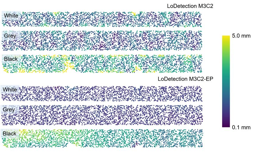
Figure 15. Significant changes for the change detection at 60 m a careful planning of scan positions is undertaken.
range and between 0◦ and 10◦ incidence angle, cropped to the
center part of the board. Points beyond the faded boundaries are In the context of time series analysis of topographic data, the
all ”True Positive” (TP) change. The points are coloured presented method is a two-fold improvement of the state of
according to their confusion matrix, i.e. whether the indicated the art: (1) Since the application of the rangefinder uncertainty
significance matches the one from the reference. model does not have a requirement for planar objects, observa-
tions of natural objects with curved or ragged surfaces are not
limited by planarity constraints. This also applies for data gaps,
where planarity measures suffer from the inexistence of data.
(2) Including the sensing process in the analysis allows the rig-
orous combination of multiple data sources, e.g. combining
airborne laser scanning data with terrestrial laser scanning data.
The individual uncertainty components of each sensing method
can be modelled and then propagated to the change quantifica-
tion.
While the findings remain to be shown with real-world, topo-
graphic data, we assume that an improved uncertainty model
allows the detection of changes that were previously discarded
as non-significant, especially on non-planar surfaces. With in-
creased acquisition frequencies and a trend towards 4D point
Figure 16. Comparison of the LoDetection between the M3C2 cloud analyses using more than 2 epochs (e.g. Anders et al.,
method and our method stemming from error propagation using 2020), these considerations become increasingly important.
the estimated model for the ranging precision (M3C2-EP). With respect to the model generation, further investigations
While our model shows a generally lower LoDetection, it is should show whether (1) models from experiments like the one
slightly higher than the baseline on the black surface material. shown in this paper can be transferred to real data or (2) the
The baseline method suffers from effects of locally lower point scanner’s uncertainty can be estimated from patches of overlap-
densities especially at the edges and close to data gaps. ping point clouds acquired from different scan positions.
References
Anders, K., Winiwarter, L., Lindenbergh, R., Williams, J. G.,
Vos, S. E., Höfle, B., 2020. 4D objects-by-change: Spatiotem-
poral segmentation of geomorphic surface change from LiDAR
This contribution has been peer-reviewed. The double-blind peer-review was conducted on the basis of the full paper.
https://doi.org/10.5194/isprs-annals-V-2-2020-789-2020 | © Authors 2020. CC BY 4.0 License. 795ISPRS Annals of the Photogrammetry, Remote Sensing and Spatial Information Sciences, Volume V-2-2020, 2020
XXIV ISPRS Congress (2020 edition)
time series. ISPRS Journal of Photogrammetry and Remote RIEGL LMS, 2012. LAS Extrabytes Implementation in
Sensing, 159, 352–363. RIEGL Software. http://www.riegl.com/uploads/
tx_pxpriegldownloads/Whitepaper_LASextrabytes_
BIPM, I., IFCC, I., ISO, I., IUPAP, O., 2008. Evaluation of implementation_in-RIEGLSoftware_2017-12-04.pdf,
measurement data—guide to the expression of uncertainty in Access: 2020-02-03.
measurement, JCGM 100: 2008 GUM 1995 with minor correc-
tions. Joint Committee for Guides in Metrology. RIEGL LMS, 2019. RIEGL VZ-2000i: Datasheet. http:
//www.riegl.com/uploads/tx_pxpriegldownloads/
Clark, J., Robson, S., 2004. Accuracy of Measurements RIEGL_VZ-2000i_Datasheet_2019-11-22.pdf, Access:
Made with a Cyrax 2500 Laser Scanner Against Sur- 2020-02-03.
faces of Known Colour. Survey Review, 37(294), 626–638.
doi.org/10.1179/sre.2004.37.294.626. Soudarissanane, S., van Ree, J., Bucksch, A., Lindenbergh, R.,
2007. Error budget of terrestrial laser scanning: influence of the
DIN, 2006. EN 300: Oriented Strand Boards (OSB) – Defini- incidence angle on the scan quality. Proceedings 3D-NordOst,
tions, classification and specifications. 1–8.
Eitel, J. U. H., Höfle, B., Vierling, L. A., Abellán, A., Wujanz, D., Burger, M., Mettenleiter, M., Neitzel, F., 2017. An
Asner, G. P., Deems, J. S., Glennie, C. L., Joerg, P. C., intensity-based stochastic model for terrestrial laser scanners.
LeWinter, A. L., Magney, T. S., Mandlburger, G., Mor- ISPRS Journal of Photogrammetry and Remote Sensing, 125,
ton, D. C., Müller, J., Vierling, K. T., 2016. Beyond 3-D: 146–155. doi.org/10.1016/j.isprsjprs.2016.12.006.
The new spectrum of lidar applications for earth and ecolo-
Wujanz, D., Burger, M., Tschirschwitz, F., Nietzschmann,
gical sciences. Remote Sensing of Environment, 186, 372–392.
T., Neitzel, F., Kersten, T. P., 2018. Determination of
doi.org/10.1016/j.rse.2016.08.018.
Intensity-Based Stochastic Models for Terrestrial Laser Scan-
Fey, C., Wichmann, V., 2017. Long-range terrestrial laser scan- ners Utilising 3D-Point Clouds. Sensors, 18(7), 2187.
ning for geomorphological change detection in alpine terrain doi.org/10.3390/s18072187.
– handling uncertainties. Earth Surface Processes and Land- Zahs, V., Hämmerle, M., Anders, K., Hecht, S., Sailer, R.,
forms, 42(5), 789–802. doi.org/10.1002/esp.4022. Rutzinger, M., Williams, J. G., Höfle, B., 2019. Multi-temporal
3D point cloud-based quantification and analysis of geomor-
James, M. R., Robson, S., Smith, M. W., 2017. 3-D uncertainty-
phological activity at an alpine rock glacier using airborne and
based topographic change detection with structure-from-motion
terrestrial LiDAR. Permafrost and Periglacial Processes, 30(3),
photogrammetry: precision maps for ground control and dir-
222–238. doi.org/10.1002/ppp.2004.
ectly georeferenced surveys: 3-D uncertainty-based change de-
tection for SfM surveys. Earth Surface Processes and Land- Zámečnı́ková, M., Wieser, A., Woschitz, H., Ressl, C., 2014.
forms, 42(12), 1769–1788. doi.org/10.1002/esp.4125. Influence of surface reflectivity on reflectorless electronic dis-
tance measurement and terrestrial laser scanning. Journal of
Jelalian, A. V., 1992. Laser radar systems. Artech House.
Applied Geodesy, 8(4), 311–326. doi.org/10.1515/jag-2014-
Kersten, T. P., Mechelke, K., Lindstaedt, M., Stern- 0016.
berg, H., 2009. Methods for Geometric Accuracy Investiga-
tions of Terrestrial Laser Scanning Systems. Photogrammet-
rie - Fernerkundung - Geoinformation, 2009(4), 301–315.
doi.org/10.1127/1432-8364/2009/0023.
Lague, D., Brodu, N., Leroux, J., 2013. Accurate 3D com-
parison of complex topography with terrestrial laser scan-
ner: Application to the Rangitikei canyon (N-Z). ISPRS
Journal of Photogrammetry and Remote Sensing, 82, 10–26.
doi.org/10.1016/j.isprsjprs.2013.04.009.
Lichti, D. D., Jamtsho, S., 2006. Angular resolution of ter-
restrial laser scanners. The Photogrammetric Record, 21(114),
141–160. doi.org/10.1111/j.1477-9730.2006.00367.x.
Mechelke, K., Kersten, T. P., Lindstaedt, M., 2007. Comparat-
ive Investigations Into The Accuracy Behaviour Of The New
Generation Of Terrestrial Laser Scanning Systems. 8th Con-
ference on Optical 3D Measurement Techniques, Vol. I., Eds.
Gruen/Kahmen, 319–327.
Pfeifer, N., Dorninger, P., Haring, A., Fan, H., 2007. Investig-
ating terrestrial laser scanning intensity data: Quality and func-
tional relations. 8th Conference on Optical 3D Measurement
Techniques, Vol. I., Eds. Gruen/Kahmen, 328–337.
Rencher, A. C., 1998. Multivariate statistical inference and ap-
plications. Wiley New York.
This contribution has been peer-reviewed. The double-blind peer-review was conducted on the basis of the full paper.
https://doi.org/10.5194/isprs-annals-V-2-2020-789-2020 | © Authors 2020. CC BY 4.0 License. 796You can also read