Installation and characterization of an electron bombardment ion source for a Space Simulation Chamber (SSC) - Karianne Dyrland FYS-3931 Master's ...
←
→
Page content transcription
If your browser does not render page correctly, please read the page content below

Faculty of Science and Technology
Department of Physics and Technology

Installation and characterization of an electron
bombardment ion source for a Space Simulation
Chamber (SSC)

—
Karianne Dyrland
FYS-3931 Master’s thesis in Space Physics – December 2016
Installation and characterization of an electron
bombardment ion source for a Space Simulation
               Chamber (SSC)

                 Karianne Dyrland

                University of Tromsø
                  December 2016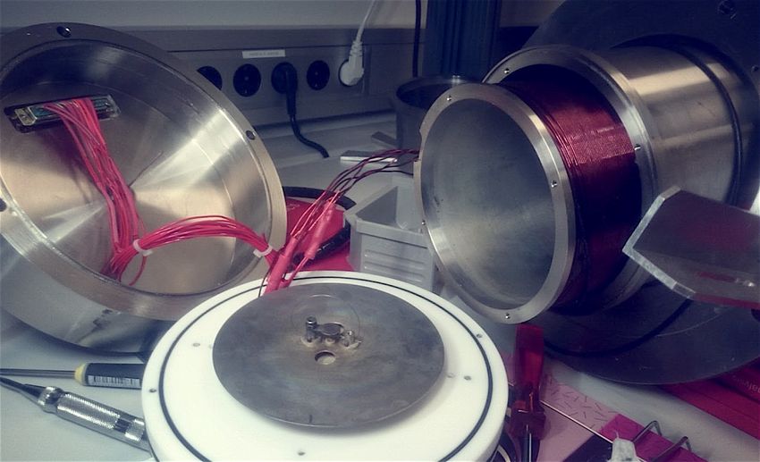
| iii

Abstract

The primary focus of this thesis is the installation and characterization of
an electron bombardment ion source for a Space Simulation Chamber (SSC).
The goal is that the chamber can be used to test satellite and sounding rocket
instrumentation, thus be capable of producing ionospheric plasma conditions,
along with an ion beam that can simulate the velocity of a rocket or satellite
relative to the atmosphere. The plasma also need to be reproductive.

First, the plasma source was prepared for operation after years in storage.
This included changing the filaments and checking the conditions of the elec-
trical connections and magnetic field. A new setup of power sources for the
different components was also done.

Second, the source was installed and characterized in the Space Simulation
Chamber. Some hang ups were encountered and solved.

Two different electrostatic probes were used to analyse the plasma. A basic
Langmuir probe, useful for finding parameters like the plasma potential, elec-
tron temperature and plasma density, and a retarding field energy analyzer
(RFEA) for finding the ion saturation current and ion energy distribution.

Some inconsistency was found in the plasma potential between the two
probes, seemingly indicating the presence of an ion beam. The plasma den-
sity is in the order of 1011 cm3 and the electron temperature is in the range
3-5 eV and can be varied using the neutralizing filament.
|v

Acknowledgements

I would like to express my sincerest gratitude to my supervisor Prof. Åshild
Fredriksen for all the help and support throughout this project.

I would also like to thank Inge Strømmesen for helping with any techical
questions or troubles in the lab, and for developing the Auro Lab Labview
systems.

I would like to thank the guys at the University of Tromsø workshop for
creating some of my almost impossible inventions.

Further on I would like to thank the Department of Physics and Technology
for the possibility to do my masters and working in a brand new lab with
teh new Space Simulation Chamber.

And lastly I want to thank my family and friends for supporting me in every
way possible through all these years at the University of Tromsø.
Contents

Abstract                                                                       iii

Acknowledgements                                                                v

Contents                                                                       vii

1 Introduction                                                                  1

2 Kaufman source                                                                3
  2.1   Principles . . . . . . . . . . . . . . . . . . . . . . . . . . . . .    3
        2.1.1   Ion production . . . . . . . . . . . . . . . . . . . . . .      4
        2.1.2   Discharges . . . . . . . . . . . . . . . . . . . . . . . . .    8
        2.1.3   Ion extraction, acceleration and neutralization . . . . . 10
  2.2   NDRE plasma source . . . . . . . . . . . . . . . . . . . . . . . 13
        2.2.1   Outer structure and gas inlet . . . . . . . . . . . . . . 14
        2.2.2   Cathode . . . . . . . . . . . . . . . . . . . . . . . . . . 14
        2.2.3   Anode and solenoid . . . . . . . . . . . . . . . . . . . . 16
        2.2.4   Grids and neutralizing filament . . . . . . . . . . . . . 17
        2.2.5   Storage tank . . . . . . . . . . . . . . . . . . . . . . . . 18

3 Experiment                                                                   19
  3.1   Preparation . . . . . . . . . . . . . . . . . . . . . . . . . . . . 19
        3.1.1   Electrical connections . . . . . . . . . . . . . . . . . . . 19
        3.1.2   Filaments . . . . . . . . . . . . . . . . . . . . . . . . . 21
        3.1.3   Magnetic flux density . . . . . . . . . . . . . . . . . . . 22
viii | CONTENTS
3.1.4 Vacuum . . . . . . . . . . . . . . . . . . . . . . . . . . 24
3.2 Installation . . . . . . . . . . . . . . . . . . . . . . . . . . . . 25
3.3 Problems and solutions . . . . . . . . . . . . . . . . . . . . . . 27
4 Measurement techniques 35
4.1 Langmuir probe . . . . . . . . . . . . . . . . . . . . . . . . . . 35
4.1.1 Principles . . . . . . . . . . . . . . . . . . . . . . . . . 36
4.1.2 Experimental setup . . . . . . . . . . . . . . . . . . . . 38
4.2 RFEA probe . . . . . . . . . . . . . . . . . . . . . . . . . . . . 40
4.2.1 Principles . . . . . . . . . . . . . . . . . . . . . . . . . 40
4.2.2 Experimental setup . . . . . . . . . . . . . . . . . . . . 42
5 Results and Discussion 45
5.1 Paschen curve . . . . . . . . . . . . . . . . . . . . . . . . . . . 45
5.2 Plasma parameters . . . . . . . . . . . . . . . . . . . . . . . . 46
5.2.1 Plasma potential . . . . . . . . . . . . . . . . . . . . . 47
5.2.2 Electron temperature . . . . . . . . . . . . . . . . . . . 50
5.2.3 Ion velocity . . . . . . . . . . . . . . . . . . . . . . . . 52
5.2.4 Ion density . . . . . . . . . . . . . . . . . . . . . . . . 52
6 Conclusion and future work 55
Bibliography 57Chapter 1 Introduction Since the discovery of the ionosphere in the beginning of the 20th century it has been of great scientific and commercial interest. The conducting layer in our atmosphere bounces radiowaves and made it first possible for us to communicate over long distance. As the second world war started there was a particularly high interest in researching the ionosphere for commu- nication purposes which led to a variety of measurement techniques being developed [1]. The two main categories are ground-based measurements and in-situ (”on-site”) measurements. Remote sensing measurements from the ground includes ionosondes, backscatter radars and lidars, while in-situ mea- surements are done by sounding rockets and satellites carrying probes and plasma instruments [1–3]. In-situ measurements are extremely useful for studying the ionosphere due to their good and accurate data. Space missions are usually very expensive and because rockets and satellites encounter harsh conditions in the lower atmosphere, it is of great interest to be able to test out the rocket and satellite equipment in ionospheric conditions before launching them into space. Thus, a large laboratory environment able to reproduce space plasma parameters along with the velocity of a rocket relative to the ionsphere is needed [4, 5]. In figures 1.1 and 1.2 (figures 4.2 and 4.4 in [1], respectively) the profiles of the electron density and temperature are shown.
2 | CHAPTER 1. INTRODUCTION

Figure 1.1: Electron density profiles   Figure 1.2: Temperature profiles in
for minimum and maximum sunspot         the ionosphere for electrons, ions and
conditions for day and night times      neutrals (figure 4.4 in [1]).
(figure 4.2 in [1]).

The main goal of this project includes installing and characterizing a plasma
source for a Space Simulation Chamber (SSC). The plasma source is an
electron bombardment ion source based on the Kaufman source originally
designed for spacecraft propulsion, and was originally at the Norwegian De-
fence Research Establishment (NDRE). The vacuum tank has previously
been equipped with an older plasma source that was contructed and de-
scribed by Hamran in 1984 (see reference [2]). A new plasma source was
built by Rein-Heggebakken et al. in 2004 (see reference [6]), based of the old
one with several new components intended to improve the source and fix the
troubles with the old one. The plasma created in the chamber will also be
measured and characterized using electrostatic probes.
Chapter 2

Kaufman source

In this chapter the history and a theorethical description of the Kaufman
type plasma source will be given along with a mechanical review of the NDRE
plasma source used in this experiment.

The Kaufman source is based on the electrostatic ion rocket engine invented
by Kaufman et al. for NASA in the early 1960’s. It was the first electric
propulsion system that succeded in-orbit testing through the SERT-I and
SERT-II missions and made the way for the Deep Space 1 which was the
first of NASA’s spacecrafts to use ion propulsion. It was then modified in
the 1980’s to become the Kaufman type ion source, also known as the electron
bombardment ion source [7–11].

2.1     Principles

The Kaufman type plasma source is an electron bombardment plasma source
where an electropositive plasma is created through impact ionization between
high velocity primary electrons emitted from a glowing filament, and a neu-
tral gas. The filament is the chamber’s cathode and is placed in the center
of the back wall of a cylindrically shaped plasma source chamber. A current
runs through the filament heating it up to emit electrons and it is biased
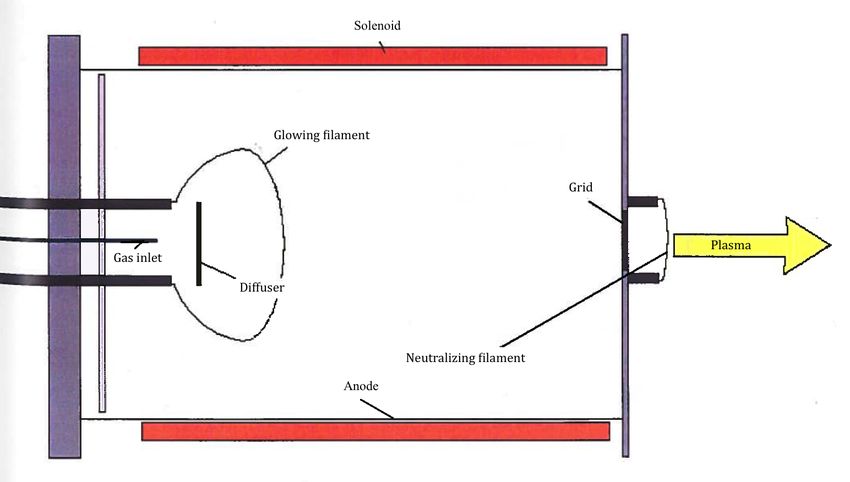
4 | CHAPTER 2. KAUFMAN SOURCE

with a negative voltage VC with respect to ground. Surrounding the cathode
lining the inner and top wall of the cylinder, is the anode which is biased
with a positive voltage VA . The applied voltages on the two electrodes serve
to attract their respectively opposite charged particles while repelling the
other. In the other end of the chamber, opposite the cathode, a negatively
biased grid extract and accelerate the ions out of the source and into a vac-
uum chamber where the ion beam is neutralized by electrons from a second
glowing filament. Electrons emitted from this neutralizing filament mix with
the ion beam to produce a quasineutral plasma able to represent the condi-
tions of the ionosphere. See figure 2.1 (from figure 5.1 in reference [6]) for a
diagram of a basic Kaufman type plasma source [2, 8–10, 12, 13].

Figure 2.1: Sketch of a Kaufmann type electron bombardment ion source
(modified from figure 5.1 in [6]).

2.1.1     Ion production

Neutral atoms are ionized through collisions with primary electrons. The
primary electrons emitted from the cathode filament are accelerated through
the surrounding negative sheath acquiring a kinetic energy Ee equal to the
potential difference between the cathode and the plasma Ee = Vp − VC . Since
2.1. PRINCIPLES | 5

most of the potential energy in the source is focused in the area of the sheath
close to the cathode filament, and only a very small potential is needed to
carry a discharge current across the plasma, the primary electrons pick up
most of the available potential energy in the plasma. This leaves the plasma
potential Vp inside the source close to the potential of the anode VA . Vp will be
slightly positive with respect to VA because the electrons have a much higher
velocity than the ions they leave the ions behind as they flow to anode. Thus
the plasma charges up with respect to the anode until enough electrons are
retained to create an equilibrium in the total flux from the filament to the
anode. The primary electron energy is therefore approximately equal to the
potential between the cathode and the anode Ee ≈ VC − VA . Figure 2.2
(figure 3.6 in [2]) shows the radial potential difference between the cathode
and the anode [2, 12, 14].

Figure 2.2: Radial plot of potential difference between cathode and anode in
plasma source chamber (figure 3.6 in [2])

To be able to ionize a neutral gas atom the primary electrons need to have
an electron energy Ee equal to or greater than the value of the first level
ionization energy WI of that gas species, i.e. the energy needed to remove a
6 | CHAPTER 2. KAUFMAN SOURCE
valence electron from that atom [12, 14, 15].
Ee ≥ WI (2.1)
For Argon we have WI = 15.7596 eV [16].
The condition required for Ee to be transferred to the valence electron of
the neutral atom, assuming a simple classical case, is determined by the
ionization or Thomson cross section given by [14].
2
e 1 1 1
π − Ee ≥ WI
σiz = 4π0 Ee W I Ee (2.2)
0 Ee < WI
where e is the elementary charge and 0 is the permittivity of free space. The
Thomson cross section has the unit m2 .
The ionization or ion production rate is given by [14]
νiz = ng σiz v (2.3)
where ng is the neutral gas density and v is the velocity. It is given in
the unit ionizations per m3 per s. Equations (2.2) and (2.3) show that the
ion production rate is inversely proportional to the electron energy. For a
full treatment of the ionization cross section and ion production rate, see
reference [14].
An effective plasma source needs an optimized ion production rate which we
can achieve by controlling the paths of the primary electrons. To do this
a large coil is wrapped around the anode cylinder creating a solenoid that
generates a nearly uniform magnetic field B = B0 in the axial direction of the
chamber. The magnetic field needs to be weak enough so that it only affects
the electrons and not the ions in the chamber, i.e. about 50 − 120 G [12, 15].2.1. PRINCIPLES | 7
This makes the electrons gyrate in circular orbits about a guiding center with
gyration or cyclotron frequency ωc and a gyration or Larmor radius rc . It
orbits perpendicular to the magnetic field keeping the electrons contained
in the radial direction while the electric field from the potential difference
between the cathode and the anode on the inner end of the chamber, and the
anode and the negatively biased inner grid on the downstream end, keep them
contained in the axial direction. Due to the collisions with the neutral gas
atoms the electrons random walk towards the anode with steps approximately
equal to the gyration radius, assuming classical diffusion. To make sure each
electron makes on average at least one collision, ionizing at least one neutral
atom, the gyroradius should be smaller than half the radius of the anode
cylinder rA [2, 8, 12, 14, 15, 17, 18].
1
rc < rA (2.4)
2
The motion of the electrons between collisions can be described by the
Lorentz force equation
dv
m = q [E(r, t) + v × B(r, t)] (2.5)
dt
where m is the particle mass, q is the particle charge, r and v are, respec-
tively, the position and velocity vectors, and E and B are the electric and
magnetic fields, respectively [14, 19].
The gyration or cyclotron frequency of the electron orbits is given by
qB0
ωc = [rad/s] (2.6)
m
and the gyration radius by
v⊥
rc = [m] (2.7)
|ωc |8 | CHAPTER 2. KAUFMAN SOURCE
where v⊥ is the speed perpendicular to the magnetic field. For electrons,
equations (2.6) and (2.7) can be rewritten into more useful units
ωc
fc,e =
2π (2.8)
≈ 2.80 · 106 B0 [Hz]
√
3.37 E
rc,e ≈ [cm] (2.9)
B0
where E is the electron energy in electronvolts and B0 is in the unit gauss
[2, 12, 14, 15, 19]. See reference [14] for a full evaluation of the electron
motion and the derivation of the gyrofrequency and the gyroradius.
As we can see from equation (2.9) the gyration radius of the electrons in
the chamber is proportional to the electron velocity and hence the ionization
rate is inversely proportional to the magnetic field strength B. The value of
B can be found for an ideal case through Ampere’s law [6]
N · Ic
B = 104 µ0 [G] (2.10)
lc
where µ0 = 4π · 10−7 VA ·· ss is the permeability of free space, N is the number
of windings of the coil, Ic is the electric current running through the coil and
lc is the length of the coil. We use the unit gauss instead of the SI-unit tesla
for practical reasons of consistency.
2.1.2 Discharges
As the electrons move through the plasma from the cathode to the anode
an electric current arises. When the electrical field between the cathode and
the anode is relatively low, this current consist of the primary electrons and
becomes saturated when all the available electrons in the source chamber2.1. PRINCIPLES | 9
are flowing to the anode. The saturation current typically has a value of
picoamperes or nanoamperes. However, if the potential difference between
the two electrodes is increased, it eventually reaches a breakdown voltage, Vb ,
high enough to supply the the electrons created in the ion production with
enough with enough energy to ionize at least one neutral atom. This leads
to an electron avalanche, i.e. a chain reaction of ionizations, and the current
will rise exponentially; this electrical breakdown is known as the Townsend
discharge [12, 15, 20–22].
The Townsend discharge is a part of the regime of dark discharges that
occur in low pressure plasmas and can be desbribed by the first and second
Townsend ionization coefficients, α and γ respectivly. The first predicts the
number of ionizations one electron makes in one meter while the second
desbribes the probability that a hot ion colliding with the cathode produces
a secondary electron [15, 20, 23].
The first coefficient α is defined by [20]
Bpd
α = Ap exp − (2.11)
Vb
where A and B are experimentally determined constants and are dependent
on saturation ionization and ionization energies respectively. p is the pres-
sure, d is the effective distance between the electrodes and Vb = Ed is the
breakdown potential.
The second coefficient B is defined by Towsend’s breakdown criterion
Rearranging equation (2.11) gives the breakdown potential [14]
Bpd
Vb = (2.12)
ln(Apd) − ln ln 1 + γ1
This is known as Paschen’s law and gives the breakdown voltage needed to
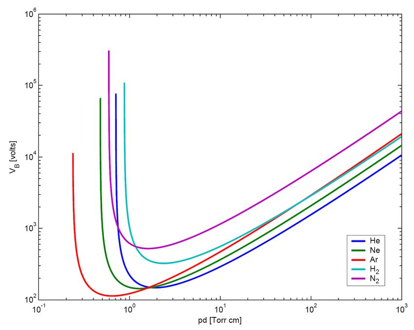
start a discharge in a gas of a specific species. Plotting Vb as a function of
pd gives the Paschen curve; a theoretical representation for several types of10 | CHAPTER 2. KAUFMAN SOURCE gases can be seen in figure 2.3 (figure from [24]). Figure 2.3: A theoretical Paschen curve for several types of gas species (fir- gure from [24], data from [14]) 2.1.3 Ion extraction, acceleration and neutralization In the downstream end of the chamber there is an isolated double-gridded hole in the anode disc. This aperture has the purpose of extracting, acceler- ating and collimating an ion beam from the plasma source. The ion beam is then neutralized by a second glowing filament electrode mounted on the outside of the source. The anode disc with its positive potential, equal to the anode potential of the cylinder wall VA , works as a screen to stop the electrons from entering the grid system. Highly mobile electrons gather and form a sheath where the potential is set a little lower than the plasma due to the higher electron
2.1. PRINCIPLES | 11

density. Ions from the more positively charged bulk plasma are attracted to
this lower potential and pulled in. On the other side of the sheath is the
inner grid, biased with a high negative potential VIG . The ions are pulled
towards this potential and accelerated to high velocity through the grid.
The acceleration of the ions is given from the potential difference between
the anode disc and the inner grid, also known as the acceleration potential
[2, 6, 12, 18]

                                V0 = VA − VIG                            (2.13)

The outer grid is known as a deceleration grid and is held at a voltage slightly
above the ground potential VOG to create a negative sheath. It has the
purpose of focusing the ion beam through deceleration. It also prevents
the backwards flow of cold ions created by charge exchange with neutrals
in the downstream end which can cause abrasion on the accelerator grid
[6, 18, 25, 26].

The ion current we are able to extract form the source is limited by both
the ion saturation current through the sheath and the space-charge limited
current flowing through the grid aperture. The ion saturation current is
defined by Bohm’s sheath criterion. This explains that the ions must have a
given velocity vB , the Bohm velocity, to pass through the sheath, assuming
a collision-less regime. If not the sheath potential will stretch out into the
plasma to set up a potential drop able to accelerate the ions up to the required
velocity vB . This is known as the presheath and is typically much wider than
the actual sheath [2, 12, 14, 15, 18].

The Bohm velocity is given by [14]

                                               1/2
                                          eTe
                               vB =                                      (2.14)
                                          mi

where e is the electron charge, Te is the electron temperature and mi is the
ion mass.
12 | CHAPTER 2. KAUFMAN SOURCE
The ion current density is given by [14].
JB = ens vB (2.15)
where ns is the density at the sheath edge.
Using the electrostatic Boltzmann relation, the sheath density to bulk plasma
density ratio is found to be [14, 15]
ns = n0 e−Vp /Te
= n0 e−1/2 (2.16)
≈ 0.61n0
where n0 is the density at the edge between the bulk plasma and the presheath
and Vp is the plasma potential.
The space separating the inner and outer grid is exclusively made up of ions.
The ion current density flowing through the grids is limited by space-charge
saturation and is governed by the Child-Langmuir law [14]
1/2 3/2
4 2e V0
J0 = 0 (2.17)
9 mi d2g
where dg is the distance between the two grids. We can clearly see that
the ion current density is strongly dependent on the potential difference and
the spacing between the two grids. We typically want a large acceleration
potential and a short separation distance [12, 18, 25].
After exiting the grids the ion beam is neutralized by a glowing filament
electrode stretched across and above the outer grid. One side of the filament
is held at approximately the ground potential. The ion beam mix with low
energy electrons emitted from the neutralizing filament through electrostatic
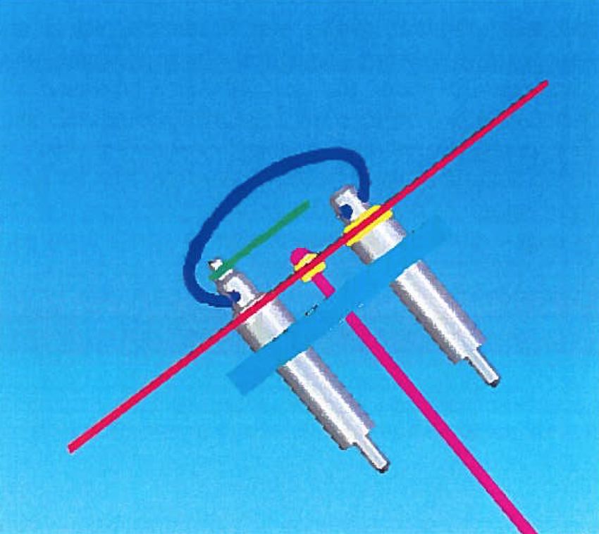
forces and we get a quasineutral beam. Without the imposed neutralization2.2. NDRE PLASMA SOURCE | 13 the ion beam would still obtain a partial neutralization by attracting electrons from the surroundings. However the benefits of neutralizing the flux directly is reducing beam divergence and prevent the build-up of large space charge potentials [8, 18, 25, 27]. 2.2 NDRE plasma source In this section a brief mechanical description of the new plasma source and its components will be given. A more detailed review is given by Rein-Heggebakken et al who constructed the plasma source in collaboration with the ionospheric team at the Norwegian Defence Research Establishment (NDRE) [6] and in the project paper reviewing the plasma source by Dyrland [28]. In figure 2.4 (from figure 7.1 in [6]) we see the main components of the source. Figure 2.4: The plasma source and the main components (based on figure 7.1 in [6]).
14 | CHAPTER 2. KAUFMAN SOURCE

2.2.1     Outer structure and gas inlet

The plasma source is a cylinder of stainless steel with the outer length and
diameter louter = 185 mm and douter = 135 mm respectively. On the outside
it has an outer structure, a back lid and a top lid both sealed to the cylinder
with O-rings. The outer structure is one of the new components added to this
redesign of the plasma source and its function is to provide a pure electric
potential in the vacuum chamber and help focusing the ions after they exit
the plasma source. On the back lid there is a terminal with wires connected
to every component of the plasma source and a gas inlet with a mount for
the gas controller, as can be seen in figure 2.4.

The plasma source uses the noble gas Argon as a propellant, it has several
benefits including a low first level ionization energy WI = 15.7596 eV , a
relatively large cross section and it is cheap and easy to get access to. A
tube leads the gas through the back lid and a 20 mm thick isolation wall,
and into the inner chamber of the plasma source where it hits a diffuser disc
spreading it evenly through the chamber [6, 16].

2.2.2     Cathode

In the inner cylinder of the source we have the cathode and the anode. The
cathode is a tantalum filament with a diameter df = 0.25 mm drawn in an
arc around the gas inlet and the diffuser disc, and is held in place by two
mounts or holders. One of the mounts is in electrical contact with the back
wall and the diffuser disc while the other one is isolated so a current can run
through the filament. The whole cathode unit consists of the components
listed in table ... and can be seen in figures 2.5 and 2.6 (figures 7.20 and 7.23
in reference [6], respectively).
2.2. NDRE PLASMA SOURCE | 15
Figure 2.5: Schematic of the cathode filament and components (figure 7.20
in [6])
Cathode components Color code in fig. 2.5
Cathode filament Navy blue
Filament mounts Silver
Diffuser disc Green
Gas tube Pink
Back wall Red
Isolation/fastening wall Light blue
Isolation Yellow
All components are made of stainless steel except for the fastening plate that
is made of the isolating plastic material PEEK, and the filament itself. The
cathode unit was designed to be taken out as a whole so the filament can be
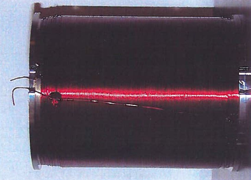
replaced easily.16 | CHAPTER 2. KAUFMAN SOURCE Figure 2.6: Picture of the cathode filament and the components (figure 7.23 in [6]) 2.2.3 Anode and solenoid The anode is the surface of the inner cylinder wall and a disc in the down- stream end of the chamber; they are in electrical contact with each other to keep them both biased at the same potential. The cylinder is made out of stainless steel and has the inner diameter dA = 116 mm and length lA = 185 mm. The anode disc is hdisc = 1 mm thick, it has a diameter ddisc = 132 mm with a hole with diameter dG = 30 mm in the middle where the grid is located. Between the inner and outer cylinder surrounding the anode is an enameled 1.12 mm thick copper wire forming a solenoid, as seen in figure 2.7 (figure 7.3 in reference [6]). A current is running through it to create a magnetic field inside the plasma source chamber. The solenoid has N = 410 windings distributed in three layers, a total length lS ≈ 160 mm and an inner diameter dS = 121 mm. See section 3.1.3 for a characterization of the magnetic field delivered by the solenoid.
2.2. NDRE PLASMA SOURCE | 17

Figure 2.7: Plasma chamber with surrounding solenoid (figure 7.3 in reference
[6])

2.2.4     Grids and neutralizing filament

This plasma source has a double grid, where the outer grid is a new feature
added together with the outer structure. The inner grid is isolated from
the anode with a disc of the isolating material PVC, as the inner grid is
going to have a large negative voltage applied to it there will be a high
potential difference between these components and no electrical contact can
be present. Another PVC disc is on the other side of the inner grid, separating
it from the outer grid that is on the outside top lid of the plasma source.
The outer grid is positively biased and has the function of grabbing high
energy primary electrons that has managed to escape through the inner grid,
as this was a problem with the old source where they would interfere with
the neutral plasma wanted in the vacuum chamber. Both grid discs have a
diameter ddisc = 132 mm and are made out of stainless steel with a circular
grid in the middle with a diameter dG = 30 mm. The grid holes have a
dh = 0.5 mm diameter and distributed with a 0.5 mm distance between
them. The isolating discs have a circular 30 mm hole in the middle equal to
18 | CHAPTER 2. KAUFMAN SOURCE

the anode disc, all grid and isolating discs are hdisc = 1 mm thick.

To get a neutral plasma electrons are added to the ion beam exiting through
the grids by a neutralizing filament stretched in a straight line across the top
of the outer grid. The filament is of the same type as the cathode filament,
a Tantalum thread with a diameter df = 0.25 mm and is held in place by
two mounts and is raised approximately 10 mm above the outer grid.

2.2.5     Storage tank

The last new addition to the source was a small miniature tank and sealing
lid. This makes it possible to test the plasma source with all components
operating without it being connected to the large vacuum tank. It is also
useful for storage purposes; when the source was stored for longer periods
exposed to air the filaments would start oxidizing and it would contaminate
the source under the next operation, however with the new miniature tank
it is possible to store it with a gas, sealed from the outside environment.

For more on the troubles of the old source, and both proposed and added
solutions, see references [2, 6, 29].
Chapter 3

Experiment

In this chapter the process of preparing, installing and configuring the NDRE
plasma source to the Space Simulation Chamber will be reviewed, along with
the hang ups and problems solved underway (for a mechanical review of the
source, see section 2.2).

3.1     Preparation

The plasma source had been in storage since it was constructed in 2004 so
a thorough check of the source had to be done before it was ready to be
installed. Wires and other parts also had to be equipped to fit our needs.

3.1.1    Electrical connections

After a decade in storage a test of the electrical system was needed to make
sure all the components still had contact with their respective outputs. The
condition of the filaments also had to be checked. To reach all the different
parts of the source and the filaments, the source had to be disassembled. The
front containing the neutralizing filament and the grids was first screwed off
to get access to the anode and cathode filament, then the back lid was taken
20 | CHAPTER 3. EXPERIMENT

off to reach the solenoid. This needs to be done with great care as the gas
tube is attached to the back wall and goes into a hole in the isolation wall
that it needs to be pulled carefully out of in a horizontal direction so it does
not bend.

To test the electrical connections a multimeter was used to check every com-
ponents to their respective output in the terminal block. The tables in appen-
dices 1, 3 and 4: Elektriske tilkoblinger, Koblingsliste D-Sub and Rekkeklem-
metabell in Rein-Heggebakken was used as a guide during the tests. All the
connections were in working as they should, and in the right place respective
to the table.

The plasma source did not come with the connector for the terminal block
and a new one had to be ordered along with the wires and plugs needed to
make a wire connected to each output on the terminal leading to a current
or voltage source. The connector arrived first and while waiting for the wires
and plugs, a couple of temporary wires were used to connect a current source
to solenoid to perform a test of the magnetic field in the chamber using a
gaussmeter with an axial probe, see section 3.1.3 for results and analysis
of this. After receiving the wires and plugs they had to be connected to
the terminal connector. The source components have ten outputs in total,
hence ten wires had to be prepared. Eight of the wires have the dimensions
Aw,1 = 1 mm2 while two have the dimensions Aw,2 = 1.5 mm2 , this is related
to how much current can run through them, a good rule of thumb is that
a 1 mm2 wire will take a current up to about 10 A while a 1.5 mm2 wire
will take up to about 15 A and so on. While it would have worked with the
smaller ones on all the components as none need currents higher than 10 A,
thicker ones were used on the solenoid so there was a possibility to go higher
if ever that is needed. Metal tips were then crimped onto one end of all
the wires and screws tighten tem into place on the connector terminal block.
Banana plugs were connected to the other end on all the smaller wires and
lugs to the two larges ones, as they were leading to a larger power supply
without any banana plug inputs. See section 3.2 for a review of the power
supplies used for the source.
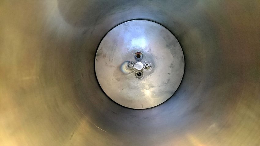
3.1. PREPARATION | 21

3.1.2    Filaments

The filaments already installed in the source were thin and old, and had to
be replaced before installation. This was done while waiting for the terminal
connector block and the wires (see section 3.1.1). As mentioned in section
2.2.2 the whole cathode unit was designed to be taken out as a whole with
a pair of long screws that fit into ridged holes next to the cathode filament.
However it did not work to pull it out of the cylinder as described and we
resorted to opening the source up from the back by removing the isolation
wall to prevent damaging any of the components as it was not clear how it
was fastened on the back.

Figure 3.1: The disassembled plasma source as the cathode filament is being
changed

The filament thread used in the source is made of tantalum and would be
preferred, but unfortunately we did not have any tantalum filament available
in the lab and it needed to be ordered. This could take a couple of weeks to
arrive and to prevent too much delay we decided to use a tungsten filament
instead as it is a very common filament used in other plasma sources. While
waiting for the tantalum filament we would then be able to install and run
prelimenary tests on the source, and change to the tantalum one when the
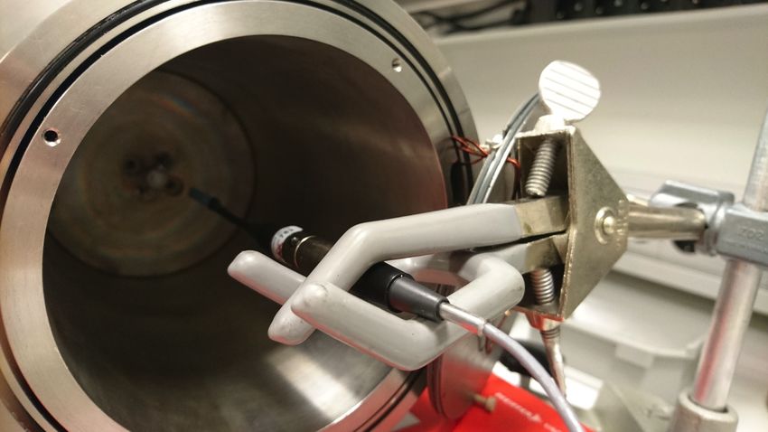
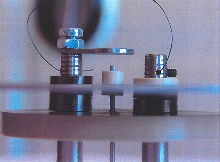
22 | CHAPTER 3. EXPERIMENT

tungsten filament needed to be replaced as glowing filaments do not have a
very long lifetime. Hamran explains in reference [2] some problems encoun-
tered while using a tungsten filament due to the fact that tungsten emits
electrons at a higher temperature and more power is needed to run it, so
some heating in the source could be expected. However, the experiment did
not call for operation over a longer period of time so we expected it would
not be a large problem for testing the basic functions of the source, as it
should still work as normal with a tungsten filament. The filament mounted
inside the anode cylinder can be seen in figure 3.2.

Figure 3.2: View inside the anode cylinder and plasma source, where the
cathode filament is streched horizontally across the diffuser disc in the middle.

After the filaments was replaced the isolation wall and back lid was reat-
tached.

3.1.3     Magnetic flux density

While the source was disassembled the magnetic field generated by the solenoid
inside the source was tested. A gaussmeter (NOTE type) with axial probe
was used to test the magnetic field strength. The probe was mounted on a
3.1. PREPARATION | 23

stand and placed approximately in the middle of, and parallel to the source
chamber, as seen in figure 3.3.

Figure 3.3: The axial probe of a gaussmeter is installed on a mount to test the
magnetic field strength, produced by the solenoid, inside the plasma source.

The magnetic field strength or magnetic flux density B was measured at
a set of predetermined values for the current running through the solenoid
Ic to get a relationship between the current and the magnetic field. We
have from equation (2.10) that the magnetic field strength is proportional
to the current so we would expect a near linear increase in field strength as
the current increases. The results can be seen in figure 3.4. A theoretical
evaluation was also done using equation (2.10) and is plotted next to the
measured values.

As we see in figure 3.4 the theoretical values and the measured values coincide
well, within ±10 G at the most. For lower values the theoretical curve and
the experimental curve are very close, ±2 G, and the curves diverge as the
current values increases. The results also fit relatively well with the test
previously done by Rein-Heggebakken et al [6] seen as the yellow plot. As
the solenoid heats up the ohmic resistance in the wire increases, which is
most likely the cause for the divergence of the theoretical and experimental
values.
24 | CHAPTER 3. EXPERIMENT

Figure 3.4: The magnetic field strength in the plasma source chamber. Blue
are the measured values and red are theoretically calculated values using eq.
(2.10). Yellow is measurements made by Rein-Heggebakken et al, values are
from figure 7.7 in [6].

3.1.4    Vacuum

Before the source is installed a test of the vacuum system was done.

The vacuum chamber has the dimensions lv = 2.16 m times dv = 0.96 m
[30]. The volume can easily be calculated to

                              V = πr2 lv
                                     d
                                = π( )2 · lv                            (3.1)
                                     2
                                = 1.5634 m3

It is equipped contains a roughing pump and two turbo pumps of the type
HiPace 800 each backed up by a Pfeiffe Penta 350 rotary vane pump. It was
first tested with one turbo pump and was able to maintain a pressure of p =
3.2. INSTALLATION | 25 1.2 · 10−5 mbar after about a weeek, which is relatively good for a chamber this large. When the second turbo pump of the same type was also connected the pumping time decreased remarkably and was able to pump down to a pressure of 1.2 · 10−5 mbar in about 7-8 hours. A pressure as low as 10−6 mbar would be preferred but this is relatively close to the ionospheric values we are looking for and in general good enough for laboratory experiments [2, 30]. Before installing the plasma source we configured the vacuum tank to fit our needs and installed a large window on the far end, directly opposite the source. We also installed a smaller one on the side of the chamber, closer to the source. These are useful for having a visual contact with the filaments in the source. 3.2 Installation The plasma source was mounted in the front door of the vacuum chamber and a mass flow controller for the argon gas was attached on the back. When the source was constructed, a custom Labview program was written by Rein- Heggebakken et al [6] to control the gas flow to the source and was hooked up to the source through the terminal on the back of the source with wires that led to a D-Sub connector for the mass flow controller. Auro lab at UiT is already equipped with a good setup and Labview program for the vacuum pumps and the mass flow control, so that was used instead for this experiment. Figures 3.5 and 3.6 show the plasma source installed in the vacuum chamber door. The first is a sideview from the outside of the chamber along with a view of the mass flow control and all wires attached. The latter show the source mounted in the door on the inside of the chamber, along with the outer grid and the neutralizing filament. All the components in the source is going to be biased at different voltages relative to a reference ground point, the solenoid and the two filaments also need a current running through them, hence several separate power sources are needed. Figure 3.7 (figure 7.32 in [6]) show an overview of the electrical
26 | CHAPTER 3. EXPERIMENT

Figure 3.5:       Sideview of source    Figure 3.6: Plasma source installed
mounted on chamber, mass flow con-      in SSC. View of neutralizing filament
troller installed                       and outer grid

potentials relative to the ground all the different components are biased to
during normal operations.

In figure 3.8 all the power sources needed to run the plasma source are shown,
the power sources and their designated voltages and currents together with
their respective components are listed in table 3.1.

The back lid of the plasma source was chosen as a ground reference point,
and a wire was attached to a screw using a lug. A banana plug was attached
to the other end to easily connect several sources in a series to the ground
point using the same wire. The complete electrical diagram for the source
can be seen in figure 3.9 (figure 4.2 in [31]).

The figure shows the structure of the plasma source with all the different
3.3. PROBLEMS AND SOLUTIONS | 27

Figure 3.7: The potentials relative to ground applied to the different source
components during normal operations (figure 7.32 in [6])

potentials and currents applied to each component, where UK is the cathode
filament current, UD is the potential applied to the cathode filament, i.e.
the discharge potential, UN is the current for the neutralizing filament and
UA , UY , UG,i , UG,y are the anode, outer structure, inner grid and outer grid
potentials respectively.

In figure 3.10 we see the chamber while in operation, with the glowing fila-
ments and a probe in front of it.

3.3     Problems and solutions

This section will review some of the hang-ups encountered during this exper-
iment along with the implemented solutions.
28 | CHAPTER 3. EXPERIMENT

Figure 3.8: The setup of the different power sources needed to run the plasma
chamber (see table 3.1 for details).

After the initial installation, the source was operated and tested a couple of
times without troubles. However after some time, an electrical connection
happened between the anode, inner grid and outer grid. The source had to
be dismounted from the vacuum chamber and disassembled. The problem
was that the PVC insulation between the grids had melted and evaporated,
leaving a conductive layer of carbon, i.e. soot, on the inside rim of all the
grid components. PVC has a melting point of 100 − 260◦ C and temperatures
in the chamber had been too hot for the plastic material, possibly due to
the tungsten filament as it emits electrons at a higher temperature than
the previously used tantalum filament [2, 32]. To gain access to the grids
and insulation the whole grid unit, or top lid of the chamber, had to be
taken apart. The PVC with the melted inner rim can be seen in figure
3.11. The best solution would be to completely exchange the PVC discs for
ceramic discs, as it is capable of withstanding very high temperatures and
3.3. PROBLEMS AND SOLUTIONS | 29

      Power source       Source type        Component           Value
     Delta Electronika
        ES 015-10          Current       Cathode filament      2−5 A
     Delta Electronika
        ES 015-10          Current     Neutralizing filament   2−5 A
     Delta Electronika
      SM 70-AR-24          Current            Solenoid         1−2 A
     Delta Electronika
      ES 0300-0.45         Voltage       Cathode filament       −50 V
     Delta Electronika
         ES 075-2          Voltage     Neutralizing filament    −1 V
     Delta Electronika
      ES 0300-0.45         Voltage             Anode            +50 V
     Delta Electronika
      ES 0300-0.45         Voltage           Inner grid        −100 V
     Delta Electronika
        ES 030-05          Voltage           Outer grid         +20 V
     Delta Electronika
        ES 030-05          Voltage        Outer structure       +20 V
Table 3.1: Power source type, designated components and their values for
normal operation of the plasma source.

is a common material used in experimental plasma physics. However, the
discs need to be 1 mm thick and have a diameter ddisc = 132 mm, which
is very thin and large for such a fragile material. Also, we had no pieces of
ceramic large enough available in the lab to try it. Instead we figured that
only the inner rim could be cut out and replaced by a ceramic inner cirle, so
that the most exposed part of the insulation would be able to stand higher
temperatures. I made a sketch and the UiT workshop was able to make it;
the final configuration is shown in figure 3.12.

While the top lid was disassembled the screw connecting the inner grid to a
wire fell off. It had not been properly fastened as it was just jammed into
a hole with no head to stop it on the other side. When the bold fastening
the wire is screwed on, naturally the screw is pulled out and disconnected.
In need of a better solution I suggested making a PEEK screw with a very
thin head, less than 1 mm to make it fit in the space between the inner and
outer grid. After drawing a sketch, the workshop managed to construct it.
Now the head stops the screw being pulled through the hole and the wire
30 | CHAPTER 3. EXPERIMENT Figure 3.9: Electrical diagram of the plasma source (figure 4.2 in [31]). connected to the inner grid is properly connected, it can be seen in figure 3.13. Also seen in figure 3.13 is the insulated wires connecting the grids to their respective power sources. When the lid is opened, e.g. when the filament needs to be changed, the enamel on the wires is very easily scraped off and it also looked like an electrical connection had occured between these wires due to a layer of soot in the surrounding area. To prevent this from being a problem the wires were insulated separately with a layer of tape. The cathode filament and the neutralizing filament also had to be replaced three times during the project. Replacing the cathode filament proves to be especially cumbersome and time consuming; the screws holding the filament are very small and is placed awkwardly on the side of the mounts instead of the top as they are for the neutralizing filament.
3.3. PROBLEMS AND SOLUTIONS | 31

Figure 3.10: The Space Simulation Chamber while operating. The light is
from the glowing filaments, and a probe can be seen right in front of it.
32 | CHAPTER 3. EXPERIMENT

                                     Figure 3.12: The inner part of the
Figure 3.11: The PVC insulation
                                     PVC insulation is replaced by a ce-
separating the grids in the plasma
                                     ramic circle so it can handle higher
source with a melted inner rim.
                                     temperatures
3.3. PROBLEMS AND SOLUTIONS | 33 Figure 3.13: The inner grid disc with the connecting wire screwed on. Also seen passing through are the two wires for the neutralizing filament and one for the outer grid.
Chapter 4

Measurement techniques

In this section the apparatus and techniques used for characterizing the Space
Simulation Chamber and the discharge plasma within are discussed. Defi-
nitions and methods for deriving important plasma characteristics, e.g. the
plasma potential, the electron temperature and the plasma density, are given.

4.1     Langmuir probe

A simple and effective instrument for measuring the parameters of a plasma is
the Langmuir probe. It is named after plasma physics pioneer Irving Lang-
muir and consists of an electrode biased with a time-dependent potential.
The probe is immersed into a plasma and a potential is sweeped from highly
negative to highly positive voltages relative to the ground, thus attracting
the ions and electrons respectively. The electric current I(VB ) is collected
as a function of the biased voltage VB and when plotted it produces what is
known as the characteristic current-voltage curve or IV-curve seen in figure
4.1 (from figure 3.6 in [2]). From the IV-curve several plasma parameters
can be determined, namely the plasma potential, the floating potential, the
electron temperature, the ion velocity, the plasma density [2, 15, 33–35]
36 | CHAPTER 4. MEASUREMENT TECHNIQUES

Figure 4.1: A theoretical IV-curve showing the current collected I(VB ) by a
Langmuir probe with a time-dependent potential sweep VB . Region A shows
the electron saturation current Isat,e , region B is the transition region and
region C shows the ion saturation current Isat,i . Vp indicates the plasma
potential, and Vf is the floating potential (edited from figure 3.6 in [2]).

4.1.1     Principles

Figure 4.1 shows three regions, A, B and C. Region C diplays the ion sat-
uration current Isat,i , region B shows the transition regime, and region A
includes the electron saturation current Isat,e . The figure also indicates the
plasma potential Vp , and the floatng potential Vf defined as the bias poten-
tial where the current contribution from the ions and the electrons are equal
[14, 33, 34]. The figure includes the ion saturation current Isat,i in region C,
the transition regime in region B, and the electron saturation current Isat,e in
region A. It also indicates the plasma potential Vp , and the floatng potential
Vf defined as the bias potential where the current contribution from the ions
and the electrons are equal [14, 33, 34].
4.1. LANGMUIR PROBE | 37
When the probe is biased with a large negative potential, the ion saturation
current is drawn. For a non-magnetized plasma when the probe is biased
enough negatively to collect only ions, Isat,i is defined by the Bohm current
density JB , given in equation (2.15), multiplied with the effective collecting
area of the probe Atot . If the plasma is magnetized the effective collecting
area is that perpendicular to magnetic field lines, meaning for a plane probe
only the area of one side is used [14, 33, 36].
The ion saturation current is given by [14]
Isat,i = eni vB A (4.1)
where A is the effective collective area probe, ni is the ion density and vB is
the Bohm velocity given in equation (2.14).
The ion saturation current can be directly measured from the IV-curve and
equation (4.1) can be rearranged to find the ion density at the probe sheath
edge [14]
Isat,i
ni = (4.2)
evB A
The plasma density at the sheath edge related to the bulk plasma density
by equation (2.16). The Bohm velocity, and hence the density, is determined
using the electron temperature Te .
First an expression for the current in this region is needed. Since the electron
saturation current is much higher than the ion saturation current due to their
small mass, Isat,i can be neglected, and we obtain [33]
k B Te
−Aene VB ≥ Vp
2m
I(VB ) =
e(VB −Vp )
(4.3)
kB Te
−Aene exp VB < Vp
2m kB Te38 | CHAPTER 4. MEASUREMENT TECHNIQUES
Assuming a Maxwellian velocity distribution in the electrons, Te can be found
in the region between the floating potential and the plasma potential, Vf <
VB < Vp . Rearrange equation 4.3 to get [33]
d e
ln|I(VB )| = (4.4)
dVB kB Te
Solve for Te to get
e dVB
Te = [K] (4.5)
kB d(ln|I(VB )|)
where we can use the relation e/kB = 11604.25 K = 1 eV to get an expression
given in electronvolts
dVB
Te = [eV ] (4.6)
d(ln|I(VB )|)
Plotting the IV-curve with a logarithmic y-axis gives a near linear curve in
the area between Vf and Vp , where the electron temperature can be procured
directly from the slope.
The floating potential Vf can be found on the curve when Isat,i = Isat,e = 0
and is expected to be relatively close to the ground potential when the plasma
is surrounded by a large grounded structure, e.g. the vacuum chamber [14].
The plasma potential Vp is defined as the maximum value of the first deriva-
tive of the IV-curve and as the zero-point on second derivative. The latter
is typically more accurate, but is often difficult to use due to too much noise
in the signal.
4.1.2 Experimental setup
A plane probe was built and custom fitted for SSC. A circular piece of con-
ducting metal with a diameter dL = 1 cm was spot wielded to the end of a4.1. LANGMUIR PROBE | 39 thin nickel wire. The wire was covered in ceramic insulation all the way up to the porbe to keep it from expanding the effective area of the probe. The vacuum chamber thoroughfeed is connected to the side of the chamber about 37 cm away from the probe, measured in a straight line along the center of the chamber. However, we wish to install the probe at about a 10 cm distance from the plasma source, meaning it needs to be brought closer. An L-shaped joint was installed at a distance of about 27 cm from the probe, then a connector was soldered on to the end of the wire and placed inside the joint. The connector can be directly connected to the thouroughfeed pole and placed approximately along the middle axis of the vacuum chamber, as seen in figure 4.2. Figure 4.2: The Langmuir probe installed in the Space Simulation Chamber The probe is controlled using a Labview data aquisition program in Auro lab.
40 | CHAPTER 4. MEASUREMENT TECHNIQUES

Here, values for the sweep range, number of steps in the sweep and offset are
implemented. A battery unit is also connected to this setup and can be used
to control the offset in the sweep as well as the program. The distributed
signal goes through a sweep amplifier and is then applied to the probe. The
current collected by the probe as a function of the sweep voltage is sent back
over a resistor, that can be easily changed to control the amplification of the
signal, and through an amplifier [33].

4.2      RFEA probe

Another simple and commonly used probe in plasma diagnostics is the retard-
ing field energy analyzer (RFEA). It collects an ion saturation current over
a potential sweep, while constantly repelling electrons. The RFEA probe is
typically used to find the ion velocity distribution, the ion energy distribution
and the ion temperature from a plasma beam [37–40].

4.2.1     Principles

The RFEA probe consists of several small grids placed inside an outer, cylin-
drically shaped, housing. The housing is usually either a metal structure
floating at the ground potential or made of some insulating material, e.g.
ceramics, leaving it at the plasma potential; the latter is often preferred as it
does not perturb the plasma as much [37]. The front plate of the probe, i.e.
the part facing the plasma beam, has a small aperture in the middle, often
covered by a grounded grid. Inside there are typically two or three grids, sep-
arated by insulated rings, and a collector plate. The first grid is the repeller
grid and is biased strongly negative to repel and stop electrons from entering
the aperture. The second is the discriminator grid which is biased with a
time-depended sweep Vg from a negative to a positive voltage, similar to that
used in the Langmuir probe, however only ions with a parallel kinetic energy
higher than Vg are able to pass through. If one chooses to apply a third grid
4.2. RFEA PROBE | 41

it is commonly biased positively and used to stop any electrons that may
have escaped through the front grid, and to contain the secondary electrons
sputtered from the collector as high energy ions collide into it. The collector
plate is often applied with a weak negative bias to attract the incoming ions
[37, 39].

The probe characteristics of an RFEA produce an IV-curve with an ion
saturation current and no electron current. Typical RFEA IV-curves (figure
6 from [38]) can be seen in figure 4.3 for different pressure values).

Figure 4.3: Typical IV-curves produced by an RFEA probe for different
values of pressure (figure 6 from [38]).

The collected ion saturation current is given by

                                         Z   ∞
                           I(v0 ) = Ae           vf (v)dv                  (4.7)
                                         v0

where A is a constant depending on the front plane pin-hole, v is the ion
velocity and f (v) is the ion velocity distribution function or the ion energy
distribution function. v0 is the minimum velocity and is given as [37, 39]
42 | CHAPTER 4. MEASUREMENT TECHNIQUES
r
2eVg
v0 = (4.8)
mi
where mi is the ion mass. From equations (4.7) and (4.8) it is clear that the
velocity distribution function is proportional to the derivative of the collected
ion current with respect to Vg . Using this we find an expression for the ion
velocity distribution function [39]
mi dI(Vg )
f (v0 ) = − (4.9)
Ae2 dVg
4.2.2 Experimental setup
The RFEA probe used in this experiment consists of a cylidrical ceramic
housing with a front plate, three grids and a collector plate inside. The
front plate is made of stainless steel and has an aperture with a diameter
dap = 4 mm. Behind it is the front grid, which should be grounded but
is not connected to anything due to faulty wires in the probe. The probe
would work well enough for our purposes without it, so we did not spend
time trying to fix this. Then we have the repeller grid, this is applied with
a voltage Vr = 70 V and is there to repel electrons. The last grid is the
discriminator with a time-dependent potential bias applied, similar to the
Langmuir probe. The collector gather the ion current of the ions able to
pass through the sweeping potential. All grids and the collector are made of
stainless steel, and all the grids have a transparency of Tg ≈ 0.5.
A schematic of the RFEA probe can be seen in figure 4.4 (adapted from
figure 3 in [37]). Both the sweep signal and the incoming probe signal go
through two separate amplifiers. The collector is biased to Vcollector = −9 V
using a battery pack.
The probe is installed in the same way as the Langmuir probe, on the
thouroughfeed with an L-shaped joint, however the probe is 10 cm shorter
than the Langmuir probe, hence it is placed at a distance at 20 cm away4.2. RFEA PROBE | 43 Figure 4.4: Sketch of the RFEA probe with the different components and materials (adapted from figure 3 in [37]). from the plasma source.
Chapter 5

Results and Discussion

In this chapter the results obtained in the experiment are presented. The
plasma parameters are derived and discussed with reference to the theory
reviewed in chapters 2 and 4, along with their significance regarding the
Space Simulation Chamber (SSC).

5.1     Paschen curve

In equation 2.12 we see the breakdown criteria for a plasma discharge to
happen in a specific gas species as a function of pressure. Measurements were
taken at different pressures where the voltage needed to make breakdown
happen was noted. Two data sets were recorded and can be seen plotted in
figure 5.1.

For the x-axis only the pressure p was used instead of the traditional product
pd, where d is effective distance between cathode and anode. This is due to
the complex geometry of our plasma source, where we have a central cathode
and a much larger cylidrically shaped anode. From the results in figure 5.1
we see a curve shaped as expected compared to the theoretical one from
figure 2.3.

The plasma is relatively reproductive as seen from the consistency of the
46 | CHAPTER 5. RESULTS AND DISCUSSION

Figure 5.1: Two sets of experimentally measured values for the Paschen curve
for an argon gas discharge in the ion source. A moving average filter and a
Savitzky-Golay filter has been applied to the curves for smoothing.

two data sets, which is a major goal in building a Space Simulation Cham-
ber. A few things to note is that when breakdown happens the discharge
grows exponentially, and since the values for the breakdown voltage are be-
ing manually adjusted and recorded the measurements of Vb should have an
error of about ±5 V . The pressure sensors has an estimated error of about
±0.5 · 10−5 mbar.

5.2     Plasma parameters

The Langmuir probe and the retarding field analyzer (RFEA) probe are
both used to determine the plasma parameters for the plasma created by
the ion source. Both probes produce a characteristic IV-curve from which
most parameters can be derived from. A set of IV-curves from the Langmuir
probe, where the plasma source is set to the voltage parameters for normal
operation given by figure 3.7, a neutralizer current IN = 3.6 A and a pressure
5.2. PLASMA PARAMETERS | 47

p = 3.5 · 10−5 mbar, is found in figure 5.2.

Figure 5.2: IV-characteristics from Langmuir probe measured at parameters
for normal operation of the plasma source, with p = 3.5 · 10−5 mbar and
IN = 3.6 A.

The Langmuir IV-curves for constant parameters are very similar, supporting
that the plasma is reproductive. Compared to the theoretical Langmuir IV-
curve from figure 4.1 we see that the electron saturation current keep rising
instead of flattening out; this is due to the fact that increasing bias voltage
also increases the effecive collection area of the probe and is expected [14].

5.2.1     Plasma potential

The plasma potential Vp can be found through derivatives of the IV-curves.
In the first derivative, the plasma potential is defined as the maximum value
while in the second derivative it is defined as the zero-point value. The latter
is usually more accurate, but harder to obtain due to very noisy second
derivatives.

In figure 5.4 the first derivatives of the Langmuir IV-curves from figure 5.2
48 | CHAPTER 5. RESULTS AND DISCUSSION

Figure 5.3: IV-curves from RFEA probe measured at normal voltage param-
eters (see figure 3.7) at different values for pressure

can be seen and the first derivatives of the RFEA IV-curves seen in 5.3 are
plotted in figure 5.5. The plasma potential found from the maximum on
each curve is listed in table 5.1. We can typically say that the error is within
±Te [eV ]n [33].

                    Probe        Data set name         Vp
                   Langmuir        Data set 1       20.4 V
                   Langmuir        Data set 2       20.4 V
                   Langmuir        Data set 3       22.2 V
                    RFEA        p = 2.5e-5 mbar     28.13 V
                    RFEA        p = 6.0e-5 mbar     26.53 V
Table 5.1: The plasma potential values obtained from the first derivative
IV-curves from the Langmuir and the RFEA probe, see figures 5.4 and 5.5.

As mentioned in section 4.2.2 the rfea probe is placed twice as far away
from the plasma source than the Langmuir probe, hence the plasma poten-
tial should decrease with distance. However, according to our measurements
seen in table 5.1 it does not. A probable explanation is that the RFEA
You can also read