Integrated water vapor and liquid water path retrieval using a single-channel radiometer
←
→
Page content transcription
If your browser does not render page correctly, please read the page content below
Atmos. Meas. Tech., 14, 2749–2769, 2021
https://doi.org/10.5194/amt-14-2749-2021
© Author(s) 2021. This work is distributed under
the Creative Commons Attribution 4.0 License.

Integrated water vapor and liquid water path retrieval using
a single-channel radiometer
Anne-Claire Billault-Roux and Alexis Berne
Environmental Remote Sensing Laboratory, Swiss Federal Institute of Technology, Lausanne, Switzerland

Correspondence: Alexis Berne (alexis.berne@epfl.ch)

Received: 2 August 2020 – Discussion started: 17 August 2020
Revised: 15 February 2021 – Accepted: 16 February 2021 – Published: 8 April 2021

Abstract. Microwave radiometers are widely used for the re-         1   Introduction
trieval of liquid water path (LWP) and integrated water va-
por (IWV) in the context of cloud and precipitation stud-           Clouds play a key, though complex, role in the atmo-
ies. This paper presents a new site-independent retrieval al-       sphere’s radiative balance and global circulation (Hartmann
gorithm for LWP and IWV, relying on a single-frequency              and Short, 1980; Slingo, 1990; Hartmann et al., 1992; Wang
89 GHz ground-based radiometer. A statistical approach is           and Rossow, 1998; Stephens, 2005; Mace et al., 2006; Mc-
used based on a neural network, which is trained and tested         Farlane et al., 2008), and cloud studies have thus been pro-
on a synthetic dataset constructed from radiosonde profiles         pelled to the forefront of climate research. One of the core
worldwide. In addition to 89 GHz brightness temperature,            challenges is the monitoring, quantification, and modeling
the input features include surface measurements of temper-          of cloud liquid water, which has a significant contribution
ature, pressure, and humidity, as well as geographical infor-       to radiative processes on a global scale. In this perspective,
mation and, when available, estimates of IWV and LWP from           highly accurate methods were developed to retrieve liquid
reanalysis data. An analysis of the algorithm is presented          water path (LWP) and integrated water vapor (IWV) from
to assess its accuracy, the impact of the various input fea-        microwave radiometer measurements, relying on the fact that
tures, its sensitivity to radiometer calibration, and its stabil-   water in its liquid and vapor phases is the main atmospheric
ity across geographical locations. While 89 GHz brightness          contributor to brightness temperatures in millimeter wave-
temperature is crucial to LWP retrieval, it only moderately         lengths outside the oxygen window. On a different note,
contributes to IWV estimation, which is more constrained by         quantifying cloud liquid water content is also relevant to the
the additional input features. The algorithm is shown to be         field of snowfall studies. Identifying the presence of super-
quite robust, although its accuracy is inevitably lower than        cooled liquid water during a snowfall event is of paramount
that obtained with state-of-the-art multi-channel radiometers,      importance to the understanding of snowfall microphysics
with a relative error of 18 % for LWP (in cloudy cases with         because it drives riming of snow particles, which in turn
LWP > 30 g m−2 ) and 6.5 % for IWV. The highest accuracy            affects the efficiency and the spatial distribution of precip-
is obtained in midlatitude environments with a moderately           itation (Saleeby et al., 2011), as well as wet deposition of
moist climate, which are more represented in the training           aerosols (Poulida et al., 1998). Improving the monitoring of
dataset. The new method is then implemented and evaluated           cloud liquid water processes is thus valuable to climatologi-
on real data that were collected during a field deployment          cal, meteorological, and hydrological applications.
in Switzerland and during the ICE-POP 2018 campaign in                 The quantitative retrieval of LWP from ground-based or
South Korea.                                                        satellite measurements of brightness temperature (TB ) at a
                                                                    single-millimeter wavelength is an underdetermined prob-
                                                                    lem. This brightness temperature results from the radiative
                                                                    contribution of gases and hydrometeors across the atmo-
                                                                    spheric column, and it depends on the vertical profile of tem-
                                                                    perature. To lift this underdetermination, state-of-the-art re-

Published by Copernicus Publications on behalf of the European Geosciences Union.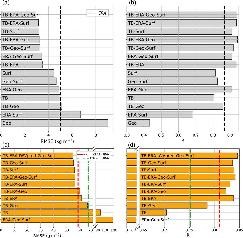
2750                        A.-C. Billault-Roux and A. Berne: IWV and LWP retrieval using a single-channel radiometer

trievals of LWP and IWV rely on multi-frequency radiome-            that relies on a single radiometer frequency. The regression is
ters, which provide TB measurements in several microwave            performed through a neural network, whose input consists of
channels. This allows for the separation of the contributions       brightness temperature at 89 GHz, as well as surface mea-
of water vapor and liquid water (e.g., Westwater et al., 2001)      surements and geographical information. Those additional
and, to some extent, the retrieval the full profile of liquid wa-   input features are shown to be especially key to the retrieval
ter content and humidity in the atmospheric column (Löhn-           of IWV. Although this new method comes with a loss of pre-
ert et al., 2004). It should be noted that IWV retrievals with      cision in comparison with state-of-the-art multi-frequency
similar accuracy are obtained using GPS sensors, as first pro-      retrievals, its advantage is to be applicable in any location
posed by Bevis et al. (1994), but this widely used technique        with a constrained uncertainty.
does not allow for the joint retrieval of LWP.                         The following section describes the data used in the differ-
   Multi-frequency instruments, however, are not always             ent steps of this study, from the design steps to the validation
available. It was shown (Küchler et al., 2017) that a radiome-      of the new method. Section 3 outlines the forward model that
ter channel at 89 GHz could be added to a W-band cloud              is used to build the synthetic dataset on which the LWP and
radar operating at 94 GHz, thus allowing collocated measure-        IWV retrieval algorithms are trained. In Sect. 4, the design
ments of radar variables and brightness temperature, paving         of the algorithms is detailed, and the results for the synthetic
the way for an improved understanding of cloud and precip-          dataset are reviewed and analyzed in Sect. 5. An independent
itation physics. Küchler et al. (2017) proposed a method to         validation of the method is presented in Sect. 6 using two
derive LWP estimates from single-frequency measurements             contrasting datasets that were collected during field deploy-
of brightness temperature, and the present study builds on          ments in Payerne (Switzerland) and in the Taebaek moun-
those findings.                                                     tains (South Korea). A summary and conclusions are pro-
   Two approaches are commonly considered for the retrieval         vided in Sect. 7.
of LWP and IWV from microwave radiometer measure-
ments, as described in Turner et al. (2007) and Cadeddu et al.
(2013). The first method relies on the reconstruction of atmo-      2     Data
spheric profiles with a physical model that is iterated until
modeled TB values match the measured ones. Although this            The present work is based on two types of data: a multiyear
method is formally the most accurate (Turner et al., 2007), it      collection of radiosonde observations across the world (for
requires more than one radiometer frequency to lift the prob-       training and testing of the retrieval algorithms) and sets of
lem’s fundamental underdetermination, and is thus not ap-           measurements from an 89 GHz radiometer deployed in var-
plicable for this study. The other way to tackle the problem        ious regions during field campaigns limited in time. Those
is to derive statistical relationships between TB s and LWP         two types of data are described below.
and/or IWV based on synthetic datasets. This approach has
been widely used for both ground-based and satellite appli-         2.1    Radiosonde dataset
cations, with varying degrees of complexity in the algorithms
(linear, quadratic, log fitting, or using neural network archi-     The design of a statistical algorithm requires a large dataset
tectures) (Karstens et al., 1994; Löhnert and Crewell, 2003;        on which to perform statistical learning. Here, this dataset
Mallet et al., 2002; Cadeddu et al., 2009). The retrieval coef-     was built using radiosonde profiles collected in over 180
ficients that are computed with this method are usually site-       stations throughout the world, available through the Uni-
specific, since they incorporate during the learning or regres-     versity of Wyoming portal (Oolman, 2020). In total, ∼ 106
sion stage the climatological features at the location of the       radiosonde profiles are used from 20 years of data (2000–
dataset. The geographical range within which a site-specific        2019). It was ensured that the data included radiosonde sta-
algorithm could be reliable is difficult to estimate, especially    tions from all climatic regions covering a wide range of alti-
if the orography of the region is complex, as highlighted           tudes (0 to 4000 m). However, lack of available data in some
by Massaro et al. (2015). In general, implementing a site-          areas inevitably results in an unbalanced dataset, wherein po-
specific algorithm in a location with a different climatology       lar and tropical areas are underrepresented compared to mid-
is likely to yield erroneous retrievals (Gaussiat et al., 2007).    latitudes, especially Europe. The possible impact on the per-
In order to implement such an algorithm at another site, a          formance of the algorithm is further discussed in Sect. 5.
new parameterization should be performed using a suitable              A quality check was performed on each of the relevant
dataset; but there might not always be enough reliable data         variables (pressure, temperature, relative humidity) through
available for this purpose. In order to avoid this lengthy pro-     the following steps: first, the minimum and maximum P (T ,
cess, and in the case of instruments that are intended to be        RH) in a given range of altitudes were extracted from each
deployed in various locations, a site-independent algorithm         radiosonde. When examining the distributions that are ob-
is more adequate (Liljegren et al., 2001).                          tained, outliers were visible, which were then removed with
   The purpose of this study is to present a new site-              a 10−4 quantile (upper and lower quantile). The atmospheric
independent method for the retrieval of both LWP and IWV            column was split into nine ranges of altitudes, and this rou-

Atmos. Meas. Tech., 14, 2749–2769, 2021                                              https://doi.org/10.5194/amt-14-2749-2021
A.-C. Billault-Roux and A. Berne: IWV and LWP retrieval using a single-channel radiometer                                        2751

tine was performed for each. In total, 6395 profiles were
flagged and removed. It was ensured that this did not re-
sult in the systematic removal of some geographical loca-
tions. Following this step, the vertical profiles of pressure,
temperature, and relative humidity were used as input to the
forward model, as described in Sect. 3. The vertical extent
of the atmospheric profiles ranges from 1 to 50 km, with a
0.25 quantile of 11 km, meaning the profiles largely cover
the lower troposphere. The vertical resolution is relatively
low (0.37 km on average).

2.2     Field deployments                                         Figure 1. Illustration of the different steps of the forward model.

In the validation stage of this work, the new method was im-
plemented using real 89 GHz radiometer data that were col-        2.2.3    ICE-POP 2018
lected during campaigns described below.
                                                                  The second dataset on which the new algorithm was tested
2.2.1    Instrument                                               was gathered during the ICE-POP 2018 campaign, which
                                                                  took place in South Korea during the 2017–2018 winter
The main instrument that was used for the implemen-               in the context of the 2018 Olympic and Paralympic win-
tation of the algorithm is the one described in Küchler           ter games in Pyeongchang. A description of the data is pre-
et al. (2017), which is here referred to as WProf. This           sented in Gehring et al. (2021). During this campaign, the
radar–radiometer system, conceived and built by Radiome-          weather was generally cold and dry; nine precipitation events
ter Physics GmbH (RPG), consists of a 94 GHz frequency-           were recorded, and occasional fog was present (about 25
modulated continuous-wave (FMCW) cloud radar with an              occurrences during the campaign timeframe). WProf was
89 GHz radiometer channel, which allows for joint active and      deployed from November 2017 to April 2018 in Mayhills,
passive retrievals of cloud and precipitation. In the data pre-   50 km southeast of Pyeongchang, at 789 m of altitude. This
sented here, WProf was deployed together with a weather           allows for an implementation of the algorithm in a context
station that provided surface measurements of temperature,        different than Payerne: i.e., in winter conditions and in a fully
pressure, and relative humidity.                                  different geographical setting located at a lower latitude and
                                                                  closer to the sea.
2.2.2    Payerne 2017
                                                                     In this case, unlike in Payerne, no independent measure-
The first dataset on which the new algorithm was evaluated        ments of LWP are available; however, radiosondes were
was collected during a field deployment in Payerne (Switzer-      launched every 3 h, thus providing a means of comparison
land) at 450 m of altitude in late spring 2017 (15 May–           for IWV retrievals, although only with a lower temporal res-
15 June). As a means of comparison, data from the Swiss           olution.
meteorological institute (MeteoSwiss) were used. The Me-
teoSwiss facilities in Payerne comprise a multi-frequency
                                                                  3     Forward model
radiometer with tipping-curve calibration, HATPRO (Rose
et al., 2005; Löhnert and Maier, 2012). This state-of-the-art     In order to develop a statistical algorithm, a large amount
instrument retrieves LWP and IWV with a nominal accuracy          of data is required to reliably perform the statistical learning
of 20 g m−2 and 0.2 kg m−2 , respectively (RPG Radiometer         phase. For this purpose, a synthetic dataset was built using
Physics GmbH, 2014). During this deployment, both WProf           the radiosonde profiles described in the previous section as a
and HATPRO measured brightness temperatures with a high           starting point. A two-step forward model was implemented,
temporal resolution of the order of a few seconds. The in-        first to identify clouds in each profile and derive the corre-
struments were located approximately 65 m apart; this dis-        sponding liquid water content, then to compute the resulting
tance is small enough that it should generally not affect the     89 GHz brightness temperature. The different steps of this
comparison of the retrieved values from the two instruments.      forward model are illustrated in the flowchart in Fig. 1.
However, in some rare cases, it is possible that a cloud would
overpass one of the radiometers but not the other, leading to     3.1     Cloud liquid model
a discrepancy in the measured brightness temperatures.
   In addition, radiosondes are launched twice daily in Pay-      To derive profiles of liquid water content (LWC) from ra-
erne by MeteoSwiss, allowing for the direct computation of        diosonde profiles of atmospheric variables, the cloud model
IWV values, which are used as a further source of validation      from Salonen and Uppala (1991) was used. Cloud boundaries
for the IWV retrieval algorithm.                                  are identified using a threshold Uc for relative humidity, with

https://doi.org/10.5194/amt-14-2749-2021                                             Atmos. Meas. Tech., 14, 2749–2769, 2021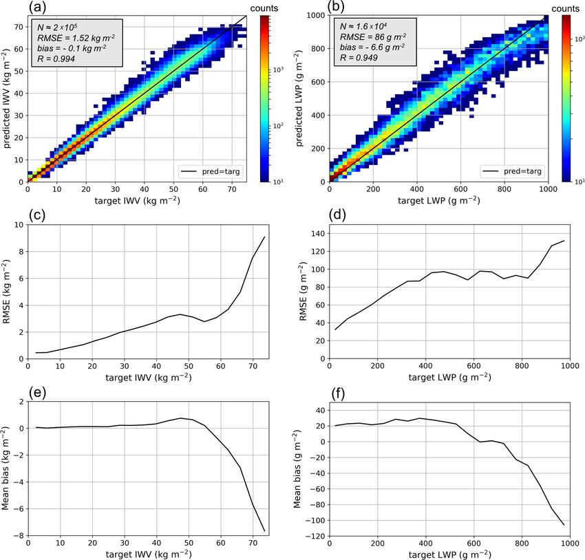
2752                         A.-C. Billault-Roux and A. Berne: IWV and LWP retrieval using a single-channel radiometer

this threshold being pressure- and temperature-dependent ac-         crowave TRansfer Model (PAMTRA; Maahn, 2015; Mech
cording to Eq. (1).                                                  et al., 2020) available at https://github.com/igmk/pamtra (last
                                                                     access: 18 November 2020). As input to the radiative transfer
Uc = 1 − ασ (1 − σ )[1 + β(σ − 0.5)]                          (1)    calculations, vertical profiles of temperature, pressure, hy-
Here, σ =   P                                                        drometeor mixing ratio, and water vapor mixing ratio are
            P0 , with P and P0 respectively denoting atmo-
spheric pressure at the current level and at the ground. Cor-        used. Gaseous absorption is calculated using the default pa-
rections from Mattioli et al. (2009) are used for the coeffi-        rameters in PAMTRA, i.e., with the model proposed by
cients α and β of the Salonen model. Within the cloud lay-           Rosenkranz (1998) and modifications from Liljegren et al.
ers, the liquid water profile is then calculated as a function of    (2005) and Turner et al. (2009). Liquid water absorption is
temperature and height above cloud base following Eq. (2):           modeled according to Ellison (2007). It should be kept in
                                                                     mind that some irreducible uncertainty remains tied to the
                     h − hb a

LWC(h, T ) = w0                 f (T ),                       (2)    choice of these parameters in the radiative transfer model.
                       hr                                               The cloud droplet size distribution (DSD) is chosen as
where f (T ) = 1 + cT for T ≥ 0 and f (T ) = exp(cT ) for            a monodisperse distribution with radius rc = 20 µm follow-
T < 0, with T in degrees Celsius (◦ C), a = 1.4, c =                 ing Cadeddu et al. (2017), and scattering calculations are
0.04 ◦ C−1 , w0 = 0.17 g m−3 , hr = 1.5 km, and h and hb re-         performed with Mie equations, assuming spherical particles.
spectively denoting the height and the height of the cloud           Let us note here that the exact choice of the DSD has lit-
base. There are some limitations to assuming a single univer-        tle impact on TB modeling as long as the droplets are in
sal cloud model, since it may fail to capture specific cloud         the Rayleigh regime for the given frequency, since the emis-
properties in certain environments; more sophisticated and           sion cross section in this regime is quasi-linearly related to
accurate models could be defined on a local geographical             the particle’s volume. When the droplet size deviates from
scale to counter this (e.g., Pierdicca et al., 2006). However,       this regime, for instance as droplets grow larger near the
given the stated objective of this study to design a non-site-       onset of precipitation, then the Rayleigh assumption falls
specific algorithm, it was considered preferable to assume a         short and higher-order terms in the Mie equations become
single universal liquid cloud model in spite of its potential        non-negligible, which alters the modeling of TB (e.g., Zhang
drawbacks.                                                           et al., 1999). This implies that the algorithm will output bi-
   A further limitation of the cloud model is related to the rel-    ased results when applied to raining cases and should not be
atively low resolution of the atmospheric profiles extracted         trusted in those circumstances. This shall be considered an
from the radiosonde data (see Sect. 2.1) that are used as an         intrinsic limitation to the algorithm.
input. This might result in a misrepresentation of the cloud            There is no clear-cut relation between LWP values and
layers in their detection and their size. In order to ensure that    the occurrence of precipitation, although the general trend
this forward model generated the least possible bias, its re-        is that higher LWP is related to more likely rain: as such,
sults were compared against LWP values from ERA5 reanal-             deviation from the Rayleigh regime is likely in high-LWP
ysis data (Copernicus Climate Change Service, 2020). Even            cases. In order to have a more rigorous grasp on when and
though the model might fail, on a given occurrence, to repro-        how this drawback might affect the retrieval, criteria from
duce the actual liquid water profile in the atmospheric col-         Karstens et al. (1994) were used. In their study, the authors
umn, it should not produce a significant bias on average. This       distinguished three types of liquid water clouds based on the
condition guarantees that the synthetic dataset that is used         value of LWC at a given altitude; for each category of cloud,
for training contains realistic – if not real – profiles, and this   a different characteristic radius is chosen for the DSD. Mie
should therefore not degrade the quality of the retrieval al-        effects can start to become an issue in the second category of
gorithm. This cloud model was chosen over other commonly             clouds (Cumulus congestus) identified for LWC > 0.2 g m−2 ;
used ones (Decker model, Salonen model without correction;           in our dataset, the atmospheric profiles in which this LWC
see Mattioli et al., 2009) because it was found to produce the       threshold is exceeded in at least one range gate have, on av-
least bias when compared to ERA5 LWP values (mean bias               erage, a total LWP ≥ 830 g m−2 , and around 2 % of the entire
of 14 g m−2 vs. 26 g m−2 (−24 g m−2 ) for the unadjusted Sa-         dataset fall into this category. Taking the third category (Cu-
lonen model (the Decker model with a 95 % threshold). In-            mulonimbus) with LWC > 0.4 g m−2 , this applies to 1 % of
evitably, when using this criterion for the choice of the cloud      the entire dataset and the average LWP threshold increases
liquid model, it is assumed that reanalysis values of LWP are        to 1400 g m−2 . Those values can serve as a benchmark to
themselves bias-free, which could be questioned, especially          identify LWP values at which Mie effects can typically con-
in extreme environments (e.g., Lenaerts et al., 2017).               taminate the retrieval. However, edge cases can also exist
                                                                     in which the total LWP is quite low, but a small layer of
3.2    Radiative transfer model                                      nearly precipitating or drizzling cloud still contaminates the
                                                                     retrieval without featuring extremely high total LWP.
Ground-level brightness temperatures (TB ) at 89 GHz are                Finally, the forward model that is presented here does not
simulated for each profile using the Passive and Active Mi-          include the contribution of ice clouds and snowfall. While

Atmos. Meas. Tech., 14, 2749–2769, 2021                                               https://doi.org/10.5194/amt-14-2749-2021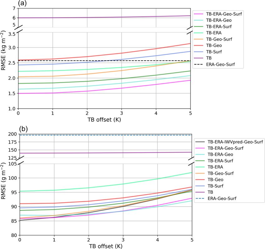
A.-C. Billault-Roux and A. Berne: IWV and LWP retrieval using a single-channel radiometer                                    2753

radiative emissions from ice and snow particles have a mi-         LWP, an additional input feature can be added, which is the
nor influence on brightness temperature when compared to           output of the IWV retrieval algorithm. The impact of each
emissions from liquid droplets and water vapor and are in          of those feature groups on the retrieval will be discussed in
general negligible, solid hydrometeors do contribute to mi-        Sect. 5.
crowave brightness temperature through the backscattering
of surface radiation. Scattering from snowfall particles is dif-   4.2   Dataset preprocessing
ficult to model accurately, but Kneifel et al. (2010) suggest
that this effect could be notable during snowfall in a way         Rain events should be excluded from the training set, since
that is highly dependent on the microphysical properties of        they are out the algorithm’s range of validity, as explained
snowfall particles and that would increase with their size.        in Sect. 3. Profiles with LWP > 1000 g m−2 are therefore re-
The present study does not take this process into account and      moved (i.e., in the range of heavy rain according to Cadeddu
could therefore yield biased results during intense snowfall       et al., 2017, and in view of the discussion conducted in
events.                                                            Sect. 3.2). The resulting dataset contains ∼ 106 profiles and
                                                                   is used for the design of the IWV retrieval algorithm.

                                                                   Further preprocessing for LWP dataset
4     Design of the IWV and LWP retrieval algorithms
                                                                   In the case of LWP retrieval, additional preprocessing is
4.1    Input features                                              needed, since the forward model produced a large majority
                                                                   of clear-sky cases. If left as such, the training phase would
When a single frequency is available for the measurement           result in a strong bias of the retrieval toward low LWP val-
of TB , the problem’s underdetermination can be partially re-      ues (a bias of ∼ 100 g m−2 for LWP > 400 g m−2 was noted
lieved by including other available information in the re-         in the development stages of the algorithm): this is a com-
trieval’s measurement vector. Adding further information al-       mon artifact in statistical learning algorithms as an effect of
lows us to disentangle IWV and LWP, which could not be             an unbalanced training set. In order to avoid this, the dataset
achieved from the sole measurement of 89 GHz TB . In this          was subsampled so that clear-sky and cloudy cases (up to
study, several categories of variables were included in the        600 g m−2 ) would be equally represented; the value chosen
input features. The first category consists of TB and higher-      for this threshold results from a trade-off between bias reduc-
order polynomials (up to fourth degree) and is expected to         tion and preservation of overall accuracy. The resulting his-
have the greatest importance in the retrieval of LWP, while        togram is shown in Fig. 2, and the LWP dataset thus contains
the other categories would likely be more correlated with          ∼ 105 profiles. In the case of IWV, the distribution is also not
IWV. The effect of higher-order polynomial terms will be           uniform, but it suffers from a much smaller asymmetry than
discussed further on. In order to simulate realistic measure-      the initial LWP dataset. After some trials, it was considered
ments, random Gaussian noise was added to the modeled              preferable to use the full IWV dataset rather than go through
brightness temperatures, with a mean and standard devia-           subsampling steps, which did not seem to bring significant
tion of 0 and 0.5 K, respectively; those values were identified    improvements in this case. It should also be noted here that
by Küchler et al. (2017) as the characteristics of the mea-        the additional preprocessing that was necessary for the LWP
surement noise of the 89 GHz radiometer. Secondly, surface         retrieval algorithm led us to design two separate algorithms
measurements are included (temperature, sea-level pressure,        rather than a single one that would retrieve IWV and LWP
and relative humidity); in the case of the radar–radiometer        at once. Indeed, while LWP retrieval is mostly relevant in
setup that is used here, a weather station is collocated, mean-    cloudy cases, IWV can show some significant variability in
ing those measurements are available at the location of the        clear-sky cases, which should therefore not be excluded from
instruments. The third class of input features comprises ge-       the training stage.
ographical descriptors: latitude, longitude, and altitude. The
day of the year is also included in this group of features as a    4.3   Statistical retrieval using a neural network
means to account for seasonal variability in atmospheric and
meteorological conditions. When available, a fourth category       After preprocessing, LWP and IWV datasets were randomly
is added to the input features with reanalysis data (precip-       split into training, validation, and testing sets (70 %–15 %–
itable water and liquid water) from ERA5 (Copernicus Cli-          15 %) and normalized using the mean and standard deviation
mate Change Service, 2020). The spatial and temporal reso-         of each input feature in the training set. The validation set is
lution of these reanalysis data is too low for them to be held     used for tuning the hyperparameters of the neural network,
as ground truth, but they can serve as a reasonable rough es-      while the final evaluation metrics are computed from the
timate and thus bring some improvements to the statistical         testing set. A densely connected neural network architecture
learning process – although it could not be included as such       was chosen over linear regression and decision-tree-based re-
in a physical model. Those four groups of features are used        trieval techniques because it was found to produce more re-
for both the retrieval of IWV and that of LWP. In the case of      liable results with higher accuracy than the former, and it is

https://doi.org/10.5194/amt-14-2749-2021                                             Atmos. Meas. Tech., 14, 2749–2769, 2021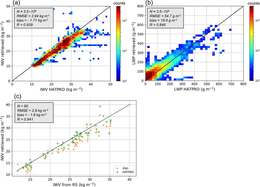
2754 A.-C. Billault-Roux and A. Berne: IWV and LWP retrieval using a single-channel radiometer
Figure 2. Distribution of the target variables (IWV and LWP in panels a and b, respectively) in the synthetic dataset after preprocessing.
less prone to overfitting than the latter. The algorithm was de-
signed using the Keras library in Python (Chollet, 2015). The
neural network was trained through mini-batch gradient de-
scent using the RMSprop optimizer, which allows for learn-
ing rate adaptation and is often used for statistical regression
problems (Chollet, 2017). As comes across from the training
curve of the LWP retrieval in Fig. 3, the training dataset is
large enough to ensure that the algorithm is not prone to over-
fitting: indeed, the error on the validation set quickly drops
with the size of the training set, then plateaus with a slight
decrease. In other words, the accuracy of the algorithm is not
limited by the amount of data used in the training stage. Fig-
ure 4 and Table 1 summarize the resulting architecture and
relevant parameters of the algorithm. These include the de-
Figure 3. Learning curves for the LWP retrieval, showing the
scription of the neural network’s structure (number of neu-
RMSE for the training and validation set with a varying training set
rons and hidden layers) and training parameters such as the size. Shaded areas correspond to the interquartile range calculated
batch size and number of epochs, i.e., the number of itera- over 50 realizations of random splitting of the dataset into training
tions through the entire dataset in the learning phase. Differ- and validation sets; bold lines are the median.
ent versions of the algorithm were trained using various sets
of input features to assess the importance of each category
(discussed below).
5 Results on synthetic dataset
performance with a single metric such as total RMSE, which
In this section, the algorithm is evaluated on the synthetic can conceal specific behaviors related to the distribution of
dataset (testing set) through different criteria. Overall, results the target variable in the dataset. Along the same line, we
are encouraging and the retrieval appears to be robust. Some emphasize that comparing total RMSE values to those from
limitations can be identified, which will be discussed here. other studies should be done carefully because they strongly
Additionally, an analysis of the impact of the various input depend on the dataset from which they are calculated. In a
features on the retrieval of IWV and LWP is conducted. similar way, Fig. 5e (f) illustrates the distribution of the mean
bias across the range of IWV (LWP) values. For reference,
5.1 Error curves the definitions of the error metrics that are used in this section
and further on are given in Table A1.
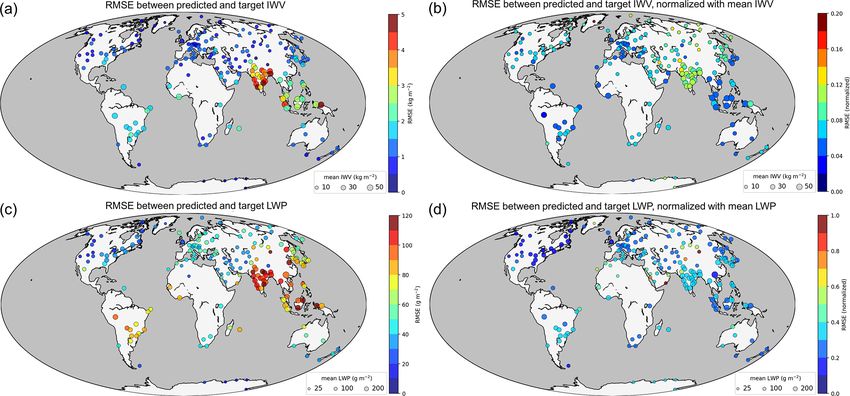
Figure 5 presents the distribution of the error on the testing Figure 6 shows how this total error, represented by the
set for the best version of the algorithm, which is the one RMSE (left panels) and the correlation coefficient (R) (right
that uses the full set of input features. In panels (c) and (d), panels), is affected by the addition or removal of input fea-
the target variables IWV and LWP, respectively, are binned tures. For each set of input features, a full tuning of the algo-
into intervals in which the root mean square error (RMSE) rithm was performed, and the results that are presented cor-
is calculated. This illustrates the behavior of the algorithm respond to those from the tuned – i.e., best – version on the
across the entire range of values rather than summarizing the testing set.
Atmos. Meas. Tech., 14, 2749–2769, 2021 https://doi.org/10.5194/amt-14-2749-2021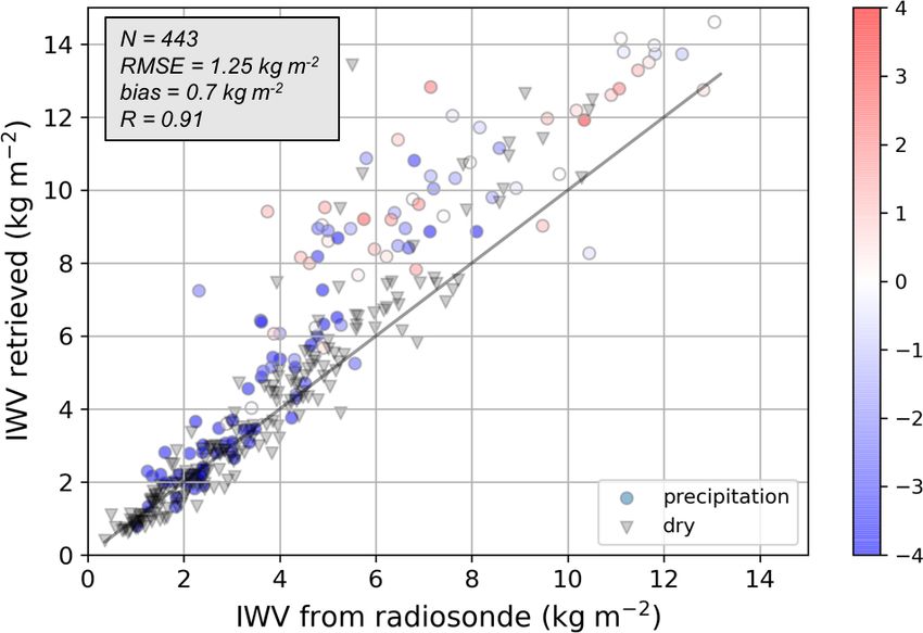
A.-C. Billault-Roux and A. Berne: IWV and LWP retrieval using a single-channel radiometer 2755
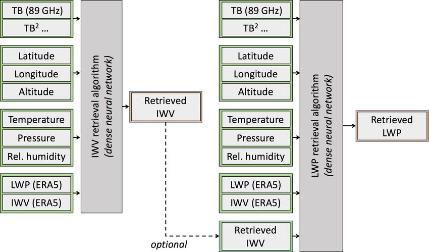
Figure 4. Structure of the retrieval algorithms. Some versions of the LWP retrieval include, among the input features, the output of the IWV
retrieval. Note that the IWV and LWP algorithms are trained on different datasets.
Table 1. Main parameters of the neural networks and training process.
Target Neurons Layers Cost function Optimizer Activation Epochs Batch size
IWV 120 7 Mean square error RMSprop ReLU 70 512
LWP 150 6 Mean square error RMSprop ReLU 90 512
5.1.1 IWV algorithm to 2.56 kg m−2 , i.e., +67 % error, which clearly shows that
brightness temperature incorporates additional relevant in-
Overall, the IWV retrieval algorithm yields an RMSE of formation into the retrieval.
1.6 kg m−2 for the testing set, which corresponds to a relative An analysis was conducted to identify the importance of
error of 6.5 %. For comparison, the ERA5 data alone have a higher-order polynomials in the algorithm, a summary of
higher RMSE (3.4 kg m−2 ) for the same dataset. Looking at which can be found in Fig. A1. It was found that the most ac-
Fig. 5a, c, and e, it comes across that the retrieval performs curate retrieval is obtained by including TB and TB2 . If higher-
quite well over the full range of IWV values, and the error order terms are added, this slightly reduces the accuracy of
distribution is relatively homogeneous. For high IWV val- the retrieval and also degrades its robustness to TB miscali-
ues, however, a significant negative bias is present (as large as bration. On the other hand, including only TB , while it makes
−6 kg m−2 ). Because such high values are underrepresented the algorithm slightly more stable, does not appear to be the
in the dataset, they are not well captured during the statistical best solution because it has lower accuracy. Hence, the re-
learning stage, which leads to a systematic underestimation. sults presented here and in the following sections are those
However, these are by definition “border” cases for which a obtained using TB and TB2 .
decrease in accuracy is to be expected.
From Fig. 6a and b it comes across that the IWV retrieval 5.1.2 LWP algorithm
is significantly improved by the addition of multiple input
features. The highest accuracy is obtained with the full set of The LWP retrieval algorithm has an RMSE of 86 g m−2 at
input t features and corresponds to an RMSE of 1.53 kg m−2 . best for the testing set (training set: 84 g m−2 , validation set:
On the other hand, including solely TB measurements in the 86 g m−2 ). This corresponds to a relative error of 29 % for the
input deteriorates the RMSE to nearly 6 kg m−2 . If only one testing set. Let us underline the fact that the subsampling per-
input feature were available, all the versions would predict formed on the dataset for the retrieval of LWP is applied to
worse results than those given by reanalysis data. Including training, validation, and testing sets: the results that are pre-
TB in the retrieval does not lead to the same leap in accuracy sented here are therefore computed on the testing set with a
as for LWP (discussed in the following subsection); however, truncated distribution – i.e., after subsampling. Additionally,
excluding TB from the input features degrades the RMSE if clear-sky cases are removed using 30 g m−2 as a thresh-
https://doi.org/10.5194/amt-14-2749-2021 Atmos. Meas. Tech., 14, 2749–2769, 2021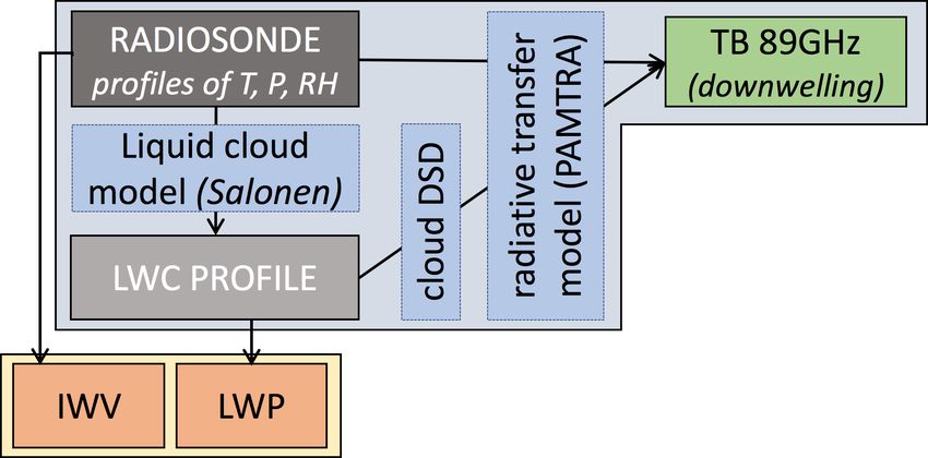
2756                          A.-C. Billault-Roux and A. Berne: IWV and LWP retrieval using a single-channel radiometer

Figure 5. Results of the retrieval algorithms for the synthetic testing dataset. The best versions of the algorithms are presented, i.e., the ones
which use the full set of input features. Panels (a) and (b) show the distribution of predicted vs. target values of IWV and LWP, respectively.
The size of the testing set is indicated (N), as are relevant error metrics (RMSE, bias, R). Panels (c) and (d) illustrate the distribution of the
RMSE across the range of IWV and LWP values, binned into intervals of 4 kg m−2 and 50 g m−2 , respectively. Similarly, panels (e) and (f)
show the distribution of mean bias across the range of IWV and LWP values.

old value, following Löhnert and Crewell (2003), the relative              likely acceptable because it would correspond mostly to rain-
error is 18 %. As already mentioned, the total RMSE values                 ing cases (light to moderate), which the retrieval does not
given here should be taken with care since they depend on                  aim to capture; yet this highlights once again that those cases
the dataset’s distribution. For comparison, when the retrieval             are out of the algorithm’s scope and that retrievals with high
is implemented on the full dataset, i.e., without the subsam-              LWP should be taken with care.
pling step, the total RMSE drops to 40 g m−2 . The RMSE                       The analysis of higher-order terms’ importance in the case
is here again rather homogeneous across the range of LWP                   of LWP retrieval shows that the best results are obtained by
values (Fig. 5d); however, there is a small bias of around                 using TB polynomials up to the fourth order (see Fig. A2),
20 g m−2 for low LWP values (visible in Fig. 5f), which are                and this does not significantly affect the stability of the re-
slightly overestimated, and there is an underestimation of                 trieval to errors in TB . Let us highlight the fact that in the
large LWP (LWP > 800 g m−2 ), with a negative bias down to                 case of a linear regression, one would expect the error to di-
−100 g m−2 . Both biases result from an effect of regression               verge when high-order polynomials are included. This is not
towards the mean, which is an intrinsic artifact of statisti-              the case here because of the saturating behavior of the neural
cal algorithms. The significant negative bias for large LWP                network. Therefore, in the results shown here and further, TB
values is enhanced by the lack of data in this range. It is                implies that TB polynomials up to the fourth order are used.

Atmos. Meas. Tech., 14, 2749–2769, 2021                                                        https://doi.org/10.5194/amt-14-2749-2021
A.-C. Billault-Roux and A. Berne: IWV and LWP retrieval using a single-channel radiometer                                                2757

Figure 6. Global error metrics (RMSE in panels a, c and correlation coefficient R in b, d) computed with the testing set for different versions
of the (a, b) IWV and (c, d) LWP retrievals. Each bar shows the result of a version whose input features are specified in the label. For
example, ERA-IWVpred-Geo-Surf corresponds to the version of the LWP retrieval algorithm that uses the following categories of input
features: ERA5 variables, IWV obtained from the IWV retrieval, geographical information, and surface measurements. The bars are sorted
with increasing RMSE. For the IWV retrieval, the accuracy of the algorithm is compared to that of reanalysis data alone (dashed lines).

   Figure 6c and d show that for LWP retrieval, input fea-                   Still, the accuracy of the algorithm drops severely when
tures other than TB only bring second-order improvements,                 no features are considered other than brightness temperature
while they were shown to be crucial in the IWV retrieval.                 (RMSE of 140 g m−2 ). This means that, although second or-
For instance, the addition of reanalysis data significantly im-           der when taken individually and somehow redundant when
proves the IWV retrieval, but only in a relatively minor way              all used together, the secondary input features are efficient in
does it increase the accuracy of LWP retrieval. In contrast,              incorporating statistical trends and climatological informa-
excluding TB from the input features leads to RMSE near                   tion into the retrieval during the training phase.
200 g m−2 and R < 0.7, i.e., to values that make the retrieval               Adding IWV prediction as an input feature to the LWP
not relevant. This highlights the fact that while environmental           retrieval has a very minor impact. For clarity, it was only in-
descriptors are well correlated with IWV, they are not suffi-             cluded in Fig. 6c in the best-case scenario and not for ev-
cient to provide a reasonable estimate of LWP, for which mi-              ery other combination of input features. This is not surpris-
crowave radiometer measurements are critical. An additional               ing, since it is itself the output of an algorithm that relies on
reason for this high dependence on TB is that LWP at a given              essentially the same input features. However, the slight im-
location can have large temporal variability due to cloud dy-             provement that is seen can be understood by recalling that
namics in the atmospheric column, which might not always                  the IWV retrieval algorithm was trained on a much larger
be captured in the time series of surface atmospheric vari-               dataset, which includes in particular a larger number of clear-
ables, nor by ERA5 models, which have a comparatively low                 sky cases (see Sect. 3).
spatial and temporal resolution.

https://doi.org/10.5194/amt-14-2749-2021                                                     Atmos. Meas. Tech., 14, 2749–2769, 2021
2758 A.-C. Billault-Roux and A. Berne: IWV and LWP retrieval using a single-channel radiometer
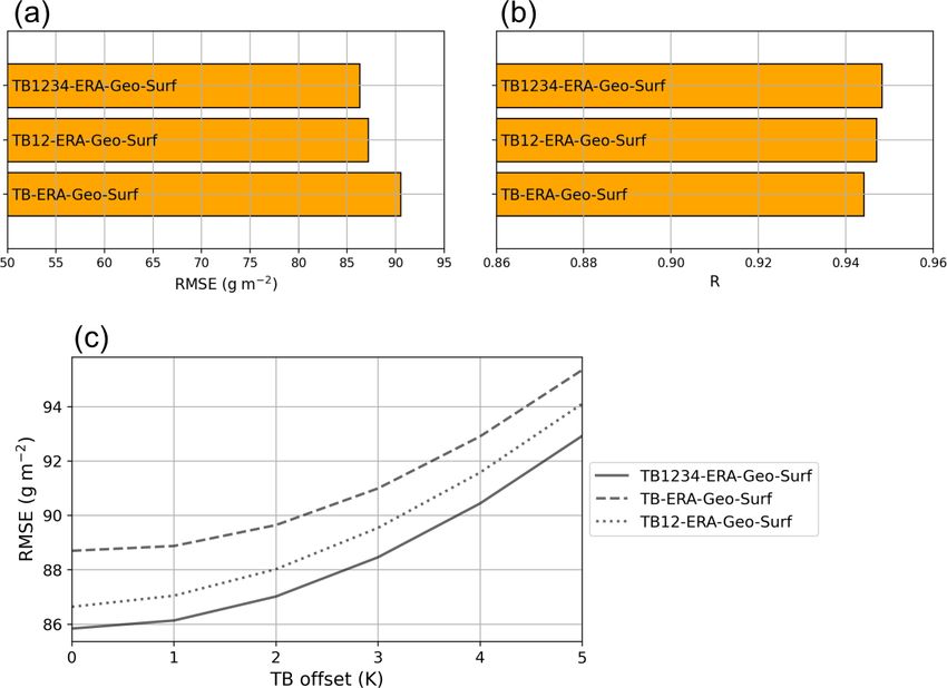
5.2 Sensitivity to instrument calibration LWP greater than 1000 g m−2 . Second, the RMSE was nor-
malized by the mean value of LWP (IWV) for each site, ex-
In order to assess the stability of the algorithm with respect to cluding low values (LWP less than 20 g m−2 , i.e., using a
potential miscalibration or calibration drift of the radiometer, conservative threshold to exclude clear-sky cases). Note that
TB offsets were virtually added to the testing dataset before this normalized error is not equal to the relative error; rather,
implementing the retrieval. Figure 7 illustrates the behavior it gives an idea of how large the RMSE of the retrieval is
of the algorithm when such a miscalibration with a constant compared to the mean values that are observed at a given lo-
offset is present (varying from 0 to 5 K). Panel (a) shows that cation.
a 5 K offset in TB results in a 30 % increase in RMSE for the From the non-normalized error (left panels in Fig. 8), it
IWV estimations, which is non-negligible. Ensuring proper can be seen that most high-latitude and midlatitude loca-
radiometer calibration thus seems crucial in constraining the tions have a constrained RMSE around 20–60 g m−2 , while
error of this retrieval. For comparison, the 89 GHz radiome- tropical sites are not as well captured, with RMSE exceed-
ter presented in Küchler et al. (2017) has a nominal accu- ing 120 g m−2 in some locations. The temperature and hu-
racy of 0.5 K after calibration. If the calibration cannot be midity conditions, as well as the strong precipitation events
ensured and if there is no means to correct for miscalibration that typically occur in those regions, are probably responsi-
(of > 3 K), it is preferable for IWV retrieval to use the algo- ble for this discrepancy. Cases with high LWP are more com-
rithm that does not rely on TB , which is shown with the black mon under such climatic conditions, and it was observed in
dashed line. Sect. 5.1.2 that the accuracy of the algorithm decreases in that
In terms of relative impact, the LWP algorithm is less af- range. Tropical climates are underrepresented in the dataset
fected (Fig. 7b) with an increase in the RMSE of less than because few data are available from this region in compari-
10 % for an offset of 5 K in TB , which makes it reasonably son with midlatitude areas: their specificity might therefore
stable to inaccuracy of TB measurements. It also appears that not be fully captured during the learning stage of the algo-
the different versions are affected in a similar way by off- rithm. This accounts at least partly for the enhanced error
set TB values. However, the algorithm that includes the pre- over the Indian peninsula and southeastern Asian islands.
diction of IWV in the input features diverges faster than the The normalized error (right panels in Fig. 8) shows that
others. This is understandable because the error in TB prop- the error is overall of the same order of magnitude across the
agates through the IWVpred input feature, in addition to the globe. However, a few regions stand out from this analysis,
TB features themselves. Therefore, in the case of uncertain which typically feature arid climates: the stations of Dalan-
calibration, more robust results would be obtained without zadgad (Mongolia), Salalah (Oman), Minfeng (China, north
including this feature. of Tibet), and Jeddah (Saudi Arabia) all have a normalized
It is noteworthy that for TB -only retrievals, the addition of error in LWP higher than 0.7 and are in the desert. In a simi-
a TB offset does not result in a large increase in the error. lar way, it appears that the IWV retrieval algorithm performs
For IWV, the addition of a 5 K offset increases the RMSE poorly – in terms of normalized error – in cold environ-
from 5.6 to 6.2 kg m−2 ; for LWP, the same offset leads to an ments where absolute humidity is low, such as in Sermersooq
increase from 139 to 142 g m−2 . This behavior is also ob- (Greenland). In such regions, the new algorithm is not sen-
served when looking at how the bias, instead of the RMSE, sitive enough to accurately capture the fine variations of at-
increases with the addition of a TB offset (not shown). In both mospheric vapor and liquid water content; if detailed studies
cases, the error increases more drastically when multiple fea- of those areas were to be conducted, more than one radiome-
tures are included than when only TB is used as input. One ter frequency would likely be necessary, along with specific
possible explanation for this effect is the following. When in- training sets on which to perform the statistical learning, as
corporating numerous input features, the algorithm is able to was done in the Arctic by Cadeddu et al. (2009).
narrow down the range of possible IWV and LWP values in
a given environmental context; in this constrained configura-
tion, the correlation and sensitivity of the retrieval to TB are 6 Evaluation in two contrasting datasets
then enhanced, leading to a stronger influence of a TB offset.
As a further step in the validation process, the algorithm was
applied to data from two campaigns involving WProf: first
5.3 Geographical distribution of the error
in Payerne, Switzerland, then near Pyeongchang, South Ko-
rea (see Sect. 2 for the full description of the datasets). In
One of the motivations of this study was to design an algo-
both cases, the output of the retrieval is compared with val-
rithm that could be used across the globe with a constrained
ues retrieved through other methods, either a multi-channel
uncertainty. Figure 8 illustrates the geographical distribution
radiometer or – in the case of IWV – radiosonde data.
of the error for both LWP and IWV retrievals using the syn-
thetic radiosonde-based dataset. Two approaches were used
to assess this error: first, RMSE values were calculated for
the entire set of data available for each location, excluding
Atmos. Meas. Tech., 14, 2749–2769, 2021 https://doi.org/10.5194/amt-14-2749-2021A.-C. Billault-Roux and A. Berne: IWV and LWP retrieval using a single-channel radiometer 2759
Figure 7. RMSE for the testing set of the different versions of the (a) IWV and (b) LWP retrieval after the addition of a constant TB offset
in the input. Dashed lines show the retrievals without TB in the input features.
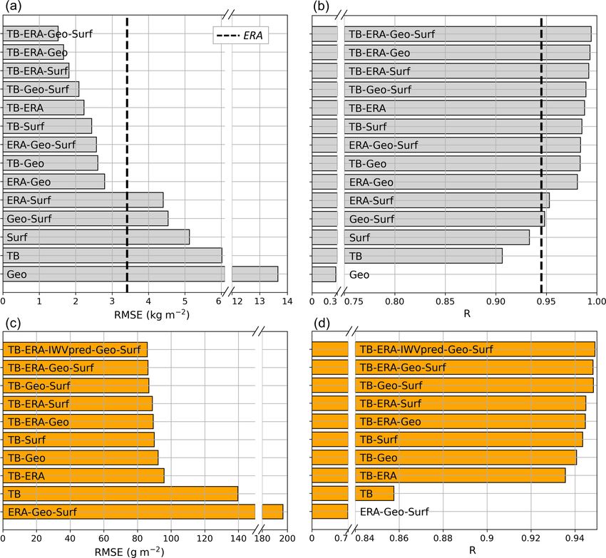
6.1 Payerne 2017 Payerne dataset matches the conclusions from the testing set
results: more features lead to an enhanced precision of the
6.1.1 IWV retrieval retrieval. The accuracy drops when only one or two groups
of input features are included, but no single group of features
seem to increase the accuracy alone. There is, however, a dif-
The results of the new IWV retrieval algorithm are com-
ference between Fig. 10b and Fig. 11b: in the latter, higher
pared to those from the MeteoSwiss operational radiometer
R (and similar RMSE) is actually obtained from the algo-
HATPRO and to the radiosonde-derived values. From Fig. 9a
rithm that does not use TB in input than with the full set of
and c it appears that the IWV retrieval has relatively limited
input features. This is at first surprising, but it was explained
spread but has a constant bias (−1.8 kg m−2 ), which is visible
by taking a closer look at the results: the algorithm without
in both the comparison against HATPRO (a) and radiosonde-
TB leads to IWV values that are more smooth and less sen-
derived measurements (c). This might be due to a bias in
sitive to short-time variations. These are not reflected in the
ERA5 data during this timeframe over the region (with a
comparison against radiosonde data, for which a 30 min av-
value of −4.1 kg m−2 ), which is visible in ERA5 records dur-
eraging was implemented.
ing the entire campaign (not shown here) and for which there
When variations over a small timeframe are considered,
is no clear explanation at this stage. This bias points to one of
the inclusion of TB improves the retrieval, as comes across
the limitations of the IWV retrieval algorithm, which is sensi-
from the comparison against HATPRO’s measurements in
tive not only to radiometer miscalibration but also to possible
Fig. 10.
biases in other input variables; this can be difficult to moni-
tor and assess – as in the case of ERA5 values in Payerne. In
spite of this, the top panels in Fig. 10 (which illustrate the er- 6.1.2 LWP retrieval
ror vs. HATPRO measurements) and Fig. 11 (error vs. value
derived from radiosounding) show that, overall, the imple- Figure 9b shows that LWP values retrieved with the new al-
mentation of the different versions of the algorithm on the gorithm are in general agreement with those obtained thanks
https://doi.org/10.5194/amt-14-2749-2021 Atmos. Meas. Tech., 14, 2749–2769, 20212760 A.-C. Billault-Roux and A. Berne: IWV and LWP retrieval using a single-channel radiometer Figure 8. Geographical distribution of the error for the synthetic dataset. Panels (a) and (c) illustrate the total RMSE for IWV and LWP, respectively. Panels (b) and (d) show the normalized error, i.e., the RMSE normalized by the mean value of IWV (LWP) at each location. For the evaluation of LWP, clear-sky and strong rainy cases are removed (LWP < 20 g m−2 and LWP > 1000 g m−2 ). The size of the disks represents the mean value of IWV or LWP at each site, while the color codes are for the error of the retrieval. to HATPRO, although a larger spread is observed than in HATPRO’s values as a reference. The algorithms perform in the IWV retrieval. A saturation effect can be seen near pre- a similar way, with slightly better results for the new algo- cipitation onset when LWP values from HATPRO reach rithm when at least one of the secondary input features is in- 600 g m−2 . Additionally, outliers are visible as vertical and cluded. We remind readers that K17A and K17B were specif- horizontal bars close to the axes, for which two hypotheses ically tuned on Payerne data, while the new algorithm was are considered. One is that the distance between the two in- tuned globally on a dataset that did not comprise radiosonde struments was big enough that in some cases a liquid wa- profiles from Payerne. ter cloud would overpass one of the two instruments but not the other. Hence, HATPRO would measure a nonzero LWP, 6.2 ICE-POP 2018 while WProf would indicate a clear sky or vice versa. Mea- surement artifacts also cannot be excluded, e.g., due to the As detailed in Sect. 2, the South Korean deployment of persistence of a liquid water film on the radome of either ra- WProf in 2017–2018 also offers an opportunity to compare diometer after precipitation or due to condensation. results from the IWV retrieval to IWV from radiosonde mea- For comparison, the method described in Küchler et al. surements. (2017) was implemented (further on referred to as K17) by The analysis of the TB time series showed that a miscali- performing a quadratic regression on a dataset consisting bration of the radiometer led to unrealistic – negative – val- solely of radiosonde profiles collected in Payerne. As pro- ues for which a correction had to be implemented through posed by the authors, a first version (K17A) relies on a mea- the addition of a constant offset to TB measurements. The surement vector consisting of TB , TB2 , and the IWV esti- value of this offset (20 K) was determined by computing the- mate from reanalysis data IWVERA5 and IWV2ERA5 . Another oretical brightness temperatures from clear-sky radiosonde version (K17B) includes only TB and TB2 . Theoretical RM- profiles and comparing them to measured TB s, following the SEs derived for those quadratic regressions for the synthetic approach of Ebell et al. (2017). This is, however, only a first- dataset (19 720 profiles) are 21 and 43 g m−2 , respectively, order correction whose output should be taken with care, es- which is similar to the values obtained by the authors from pecially after the analysis in Sect. 5.2, which underlined the radiosonde data from De Bilt (the Netherlands), i.e., 15 and importance of TB accuracy for IWV retrieval. 44 g m−2 . After this correction, the IWV retrieval gives coherent re- K17A and K17B were applied to the Payerne campaign sults (see Fig. 12), with a total RMSE that is slightly lower dataset, and their results are compared to those from the new than that obtained for the testing dataset (1.25 kg m−2 ). The algorithm in Fig. 10. The error metrics are calculated using best results are found when several input features are in- Atmos. Meas. Tech., 14, 2749–2769, 2021 https://doi.org/10.5194/amt-14-2749-2021
A.-C. Billault-Roux and A. Berne: IWV and LWP retrieval using a single-channel radiometer                                           2761

Figure 9. Comparison of (a) IWV and (b) LWP retrieved over Payerne with the new algorithm using the full set of input features against the
retrieval from the MeteoSwiss radiometer HATPRO. Panel (c) shows IWV retrieved from the new algorithm and from HATPRO against that
from radiosonde measurements; a 30 min time averaging is used for radiometer measurements. The size of the dataset is indicated (N ), as
are relevant error metrics (RMSE, mean bias, R).

cluded and drop severely when no secondary input features              since the geographical parameters are constant, the tempo-
are used, which corresponds to the results for the synthetic           ral variability is that of the reanalysis data, and therefore
dataset presented in Sect. 5. The algorithm largely relies on          the correlation coefficient of the retrieval is close to that of
non-radiometric features, and this is even more the case in            ERA5 data alone. Let us highlight the fact that although re-
cold and dry environments like that of ICE-POP, where IWV              analysis data outperform the retrieval for ICE-POP, this was
is low. In fact, slightly better results are obtained with all in-     not the case in Payerne nor in the full radiosonde dataset, for
put features except brightness temperature. The miscalibra-            which the algorithm has a higher accuracy than ERA5 values.
tion of the radiometer, which may not have been perfectly              Possibly, the dry and cold weather that was observed during
corrected by the addition of a constant offset, might empha-           the ICE-POP campaign featured little short-term variability
size this error. This also corresponds to what was noted in            and was associated with stable atmospheric conditions that
Payerne: when the results are averaged over 30 min, bright-            were particularly well captured in ERA5 reanalyses. Snow-
ness temperature brings little, if any, improvement to the re-         fall events during the campaign, as well as occasional fog,
sults. TB is relevant when a higher temporal resolution is             can also bias the retrieval by enhancing brightness tempera-
considered (see Sect. 6.1.1) – for which no comparison was             ture.
available during ICE-POP – or when ERA5 data are sig-                     The analysis of the ICE-POP data was taken a step further
nificantly off. In this case, however, it comes across from            to explore the latter point. It appears that the IWV retrieval
Fig. 12 that the algorithm is consistently outperformed by             is most reliable in non-precipitating or cold conditions, i.e.,
ERA5 products: they have both a lower RMSE and a higher                when little liquid water is expected in the column. To visual-
R, which makes the algorithm less relevant for the study of            ize this, periods with no precipitation or fog are identified us-
this specific campaign. The high accuracy of ERA5 data dur-            ing WProf’s radar measurements as time steps with low radar
ing ICE-POP also explains the high correlation coefficient of          equivalent reflectivity (Ze < −10 dBZ) in the lower gates
the retrieval that uses ERA5 and geographical input features:          (first kilometer above the radar), and temperature time series

https://doi.org/10.5194/amt-14-2749-2021                                                  Atmos. Meas. Tech., 14, 2749–2769, 2021
2762                          A.-C. Billault-Roux and A. Berne: IWV and LWP retrieval using a single-channel radiometer

Figure 10. Error of the new retrieval algorithms over Payerne compared to HATPRO retrievals. In panels (a) and (c) the RMSE of IWV and
LWP is respectively calculated for different versions of the algorithm. Similarly, R is shown in (b, d). Each bar shows the result of a version
whose input features are specified in the label. In panels (a) and (b), the black dashed line shows the error of IWV from ERA5 reanalysis
data. In (c, d), the dashed lines present the results from K17A and K17B, as defined in the text.

are provided by the weather station coupled to WProf. Fig-                7   Summary and conclusions
ure 13 shows the scatter plot of the error – for the algorithm
that includes all input features – color-coded to differenti-             A new site-independent method was designed for the re-
ate dry from precipitating or fog conditions: black triangles             trieval of LWP and IWV from a single-channel ground-based
correspond to dry time steps and circles to time steps with               radiometer. In addition to 89 GHz brightness temperature,
Ze > −10 dBZ, with their color indicating surface tempera-                additional input features were used for the retrieval, such
ture. The algorithm yields a larger bias in rain – as was ex-             as surface atmospheric variables (temperature, pressure, and
pected in the design steps of the algorithm (Sect. 3) – but also          humidity) and information on the geographical location and
during snow events with relatively warm temperatures close                season. A neural network architecture was chosen for the sta-
to or slightly above 0 ◦ C (Fig. 13). Changes in the dielectric           tistical learning.
properties of snowflakes during the melting process can ex-                  Training and testing were performed on a synthetic dataset
plain this increased error; additionally, the process described           that was built using radiosonde profiles worldwide. The ge-
by Kneifel et al. (2010) and that was recalled in Sect. 3 sug-            ographical distribution of the error shows that the algorithm
gests that snowfall events with large snow particles (typi-               performs better in midlatitudes and regions with a moderate
cally present with relatively mild temperatures) could have a             climate than in areas with extreme climates (either arid or
non-negligible contribution to brightness temperature, which              very moist), which include both tropical and polar regions
might explain the enhanced error in those cases.                          that are not well represented in the training dataset due to
                                                                          lack of available data. Also, the forward model that was used

Atmos. Meas. Tech., 14, 2749–2769, 2021                                                      https://doi.org/10.5194/amt-14-2749-2021
You can also read